Low-cost localization service for roadside sensors based on passive information

Abstract

The remote surveillance and tracking of vehicles on roads is generally achieved by means of a network of sensors deployed along the roadside. The effectiveness of such networks depends fundamentally on the precision with which the sensor locations are known Global Positioning Systems provide an effective means of pinpointing the sensor locations. However, such systems are expensive, and are therefore impractical for large-scale sensor deployment. Accordingly, this paper proposes a low-cost sensor localization service based on binary detection information and a road map. In the proposed algorithm, the sensors are classified as either intersection nodes or non-intersection nodes in accordance with the stochastic characteristics of the binary detection information. Having identified all of the non-intersection nodes along each road segment, the intersection nodes are connected with the non-intersection nodes by means of a clustering technique. Finally, the positions of the roadside sensors are identified by mapping the clustered sensors to the known road map. The simulation results show that the proposed algorithm outperforms existing localization algorithms reported in the literature.

Keywords

Car surveillance localization service clustering roadside sensor location binary detection

1. Introduction

The localization of roadside sensors is an important requirement for the effective functioning of road network applications such as remote vehicle surveillance and tracking [1,7,10]. Before locating these roadside sensors, an efficient sensor deployment is needed and some works use unmanned aerial planes to drop wireless sensors onto the target road network [5,22]. Existing localization schemes are typically based on information such as the vehicle id, the vehicle speed, or the vehicle direction. However, acquiring this information requires the use of sophisticated hardware such as GPS transmitters/receivers or ranging devices. Such equipment is expensive, and is therefore impractical for large-scale sensor deployment. Accordingly, a requirement exists for alternative, low-cost solutions for roadside sensor localization.

Nowadays, there are many existing localization schemes, which are usually developed based on either range measurement techniques [23–25,27] or the sharing of connectivity information [20,21]. One of the most common range measurement techniques, Time-difference-of-arrival (TDOA) [25], uses a location-support system to facilitate in-built, mobile, location-dependent applications. In such an approach, mobile or static sensors determine their locations by analyzing the temporal characteristics of the signals received from multiple beacons distributed throughout the target environment. For the sharing of connectivity information, the Ad Hoc Positioning System proposed in [20], some of the sensors have the ability to determine their locations directly (e.g., via GPS), while the remainder determine their locations by analyzing the Angle of Arrival (AOA) of the signals emitted by the sensors with a known location. Besides, in [3], the authors proposed a RF-based localization scheme for small, low-cost devices in unconstrained outdoor environments. In the proposed approach, the receivers (sensors) localized themselves with a high confidence to the centroid of a set of proximate reference points using a simple connectivity metric. In Approximation Point-In-Triangulation Test (APIT) [13], a range-free localization scheme, the network environment is isolated into overlapping triangular regions between a small number of GPS-equipped devices (anchors). By examining the triangular regions to which they belong, the sensors are able to approximate the area of the network within which they reside. By further inspecting the coordinates of the triangle vertices (i.e., the anchors), the sensors reduce the diameter of the estimated area in which they reside, and obtain a good location estimate as a result. In [17], the authors proposed a range-independent localization algorithm designated as SeROC to enable sensors to determine their position in un-trusted environments with the assistance of a small number of trusted entities. In [19], a probabilistic localization method based on robust quadrilaterals was proposed for sensor localization without the need for beacons or anchors.

In addition to the methods presented above, the literatures also contain various active event-driven localization algorithms [26,31,32,38]. Basically, these algorithms create artificial events using an event scheduler and then analyze these events in order to estimate the sensor location. However, for such algorithms to function, the sensors must be fitted with special hardware such as event generators or optical retro-reflectors [32,38]. As a result, while such methods yield an effective localization performance, they are economically unviable for large-scale deployment. In addition, many of the schemes presented in the literatures [3,13,17,19–21,23–25,27] require the sensors to exchange local information in order to derive their global positions. Thus, to achieve a satisfactory localization performance, a dense deployment of sensors is required. However, in many environments, such a deployment is not feasible due to cost constraints or difficulties in physically deploying the sensors. As a result, the localization performance of these schemes is inevitably degraded. Recently, other more localization algorithms in sensor networks are proposed and please refer to literatures [4,6,8,9,18,28,30,33,34,36,37].

For sensor localization in sparse networks, the literatures contain two basic proposals. In the first approach, mobile anchor nodes fitted with GPS technology follow a predetermined route through the network, and the sensors determine their locations from the beacon messages broadcast by these anchors as they travel [11,12,29]. In the second approach, a distance vector (DV) exchange is performed such that all of the nodes in the network can obtain their minimum distance (in hops) to the anchors. The average hop size is then estimated and deployed as a correction to all the nodes in the network. Finally, the unknown sensor positions are estimated via triangulation or minimum likelihood estimation [35].

In our study, we focus on car surveillance or target tracking on roads (e.g. battlefield), in which sensors are commonly deployed on the roadside. The location of road-side sensors is an important determinant of the effectiveness of such a sensor surveillance system. The effectiveness of such networks depends fundamentally on the precision with which the sensor locations are known GPS or vehicle identification device, ranging device or so forth provide an effective means of pinpointing the sensor locations. However, such systems are expensive, and are therefore impractical for large-scale sensor deployment. Accordingly, this study proposes a low-cost localization service for roadside sensors without the need for GPS or vehicle identification devices. In the proposed approach, the roadside sensors perform a binary detection of the passing vehicles and the sensor locations are then identified on a known map via a statistical analysis of the detection timestamps. It classifies sensors as intersection or non-intersection nodes by analyzing the stochastic characteristics of the obtained information on the binary detection of vehicles. After identifying the non-intersection nodes for each road segment, the algorithm connects the intersection nodes with the non-intersection nodes by means of clustering. Furthermore, the proposed algorithm filters the clustered sensors by using a road map, and thereby, determines the positions of road-side sensors.

The remainder of this paper is organized as follows. Section 2 presents the background to the localization problem considered in this study and describes the related research. Section 3 describes the localization scheme proposed in this study. Section 4 compares the localization performance of the proposed scheme with that of an existing localization method by means of numerical simulations. Section 5 discusses the performance of the proposed localization algorithm in large-scale networks and makes a comparison of the computational complexities of APL and the proposed algorithm. Finally, Section 5 presents some brief concluding remarks.

2. Background and related work

2.1. Time difference on detection

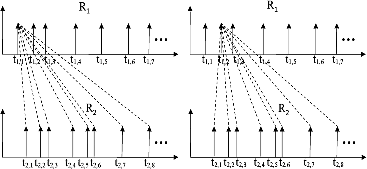
In the Time Difference on Detection (TDOD) algorithm [14], sensor localization is achieved by estimating the time difference on detection between two neighboring sensors. In their proposed approach, the vehicle arrival patterns recorded by any sensor are statistically maintained at the neighboring sensors, and the road segment length, i.e., the distance between the two sensors, is estimated from the time taken by the vehicles to move between the two sensors (i.e., the movement time) and the speed limit of the particular road segment.

Fig. 1.

Time difference on detection operation for sensors $R_{1}$ and $R_{2}$ .

Fig. 2.

Time difference for two nighobring sensors.

Figure 1 shows the TDOD operation performed at the localization server for two sensors $R_{1}$ and $R_{2}$ . The TDOD operation for the two timestamp sets $T_{p}$ and $T_{q}$ obtained from sensors $R_{p}$ and $R_{q}$ , respectively, is defined as follows: $\begin{matrix} (1) & d_{x y}^{p q} = | t_{p x} - t_{q y} | \end{matrix}$ where $t_{p x} \in T_{p}$ for x is the xth timestamp of timestamp sets $T_{p}$ and $t_{q y} \in T_{q}$ for y is the yth timestamp of timestamp sets $T_{q}$ . The passing-vehicle detection counted in each time difference value is computed using the following quantized function: $\begin{matrix} (2) & {\hat{d}}_{x y}^{p q} = q (d_{x y}^{p q}) \end{matrix}$ where q transforms $d_{x y}^{p q}$ to a discrete value. The granularity of the time difference value defines the interval between two neighboring quantization levels. The frequency represents the count of the discrete time difference value, as shown in Fig. 2.

Once the localization server has performed TDOD estimation for the two timestamp sequences received from $R_{p}$ and $R_{q}$ , the quantization level of the highest frequency time difference value is taken as the movement time of the vehicles between the two sensors. That is, $\begin{matrix} (3) & {\hat{d}}^{p q} \leftarrow arg max_{q_{h}} f (q_{h}) \end{matrix}$ where f is the count (i.e., frequency) of quantization level for $h = 1, \dots, k$ , and k is the number of quantization levels. The length of the road segment between the two sensors is then calculated as the product of the movement time and the mean vehicle speed along the segment.

2.2. Autonomous passive localization

In the Autonomous Passive Localization (APL) scheme [14], the distance between each pair of roadside sensors is estimated from vehicle-detection timestamps, and a virtual graph is then constructed composed of sensor IDs (i.e., the vertices) and distance estimates (i.e., edges). The graph is then mapped to the corresponding road map in order to estimate the physical position of each sensor. For APL to function correctly, the sensors must be time-synchronized and have a binary vehicle detection capacity such that ranging or GPS devices are not required. Furthermore, the road map corresponding to the observed network must be available to the APL server. Finally, the mean vehicle speed must be close to the speed limit of the road.

In APL, each sensor sends its vehicle-detection timestamps together with its ID to the APL server. The server then performs a TDOD operation for all the sensors and estimates the distances between each pair of sensors. The APL server then estimates the movement time of the edge (i.e. distance between two arbitrary nodes) or path as the maximum count of the TDOD operation for the corresponding nodes. Finally, by assuming a mean vehicle speed close to the speed limit of the road, the APL server calculates the length of the edge or path between the two sensors.

In the subsequent fine-tuning phase, APL uses a minimum spanning tree and the relative deviation errors to filter out the less likely paths and it constructs a virtual graph comprising all possible edges. Typically, the edge estimates are more accurate than the path estimates. In addition, the APL algorithm uses the ratio of the standard deviation to the mean of TDOD to eliminate erroneous distance estimates when constructing the virtual graph. Finally, the physical location of each sensor is determined by mapping the permutation matrix of the reduced virtual graph onto the real graph (i.e., the road map).

2.3. Statistical tests

A statistical test [15] is a mechanism for making quantitative decisions about a process (or set of processes). Through the analysis of experimental data, a statistical test can determine whether or not there is sufficient evidence to reject a particular hypothesis about a given process. In the localization method proposed in this study, statistical tests are used to examine the similarity between the parameters of the observed populations.

When performing a statistical test, it is first necessary to clearly state the null hypothesis H0 and the alternative hypothesis H1 (i.e., the hypothesis contrary to the null hypothesis). Only when the sample information provides sufficient evidence can the null hypothesis be rejected. The level of significance α, which represents the probability that the null hypothesis will be rejected, indicates the risk taken by rejecting the null hypothesis. The lower the value of α, the more accurate the test. A critical value which represents the boundary for the possible rejection of the null hypothesis can be determined from the level of significance. If the test statistic is less than this critical value, the null hypothesis is rejected. Consequently, the test itself can determine whether or not the null hypothesis should be rejected.

When performing statistical tests, a so-called Type 1 error may occur, in which the null hypothesis is incorrectly rejected (i.e., false positive error). The probability of a Type I error is equal to the significance level, α. That is, $α = P$ (Reject H0|H0 true). Alternatively, a Type II error may occur, in which the null hypothesis should be rejected, but is erroneously accepted. The probability of a Type II error is equal to the power of the test, β. That is, $β = P$ (Fail to reject H0|H0 false). In general, for any given sample size the effort to reduce one type of error results in increasing the other type of error.

The present study utilizes two statistical tests to examine the parameter relationship of the observed vehicle-detection timestamps. Specifically, the F-test [15] is used to check for a statistical difference in the variances of two arbitrary TDOD values. In addition, the T-test [15] is used to check for statistical differences in the means of the vehicle inter arrival times at two arbitrary sensors.

3. Sensor localization scheme with passive information

3.1. System model

The proposed localization scheme is based on the following assumptions: (1) the roadside sensors have no ranging or GPS devices and can sense vehicles only via binary detection. (2) The sensors are sparsely deployed and they are connected via off-the-road sensors. (3) The roadside sensors are uniformly distributed. (4) No two roadside sensors can sense one another. (5) The sensors are time-synchronized at the millisecond level. (6) Each sensor detects passing vehicles and generates a corresponding vehicle-detection timestamp in the form of a tuple $(R_{i}, T_{j})$ consisting of a sensor ID $R_{i}$ and timestamp $T_{j}$ . (7) The server collects the timestamp information from all of the sensors and performs a statistical analysis of the timestamp information in order to achieve sensor localization. (8) The road map of the target area is available to the server, and thus the real graph can be constructed. (9) Different vehicles move at different speeds in the observed road network. However, each vehicle maintains a constant speed as it moves, and this speed is lower than the speed limit assigned to the road segment.

The following terms are defined in order to facilitate a description of the proposed localization algorithm:

Intersection nodes:

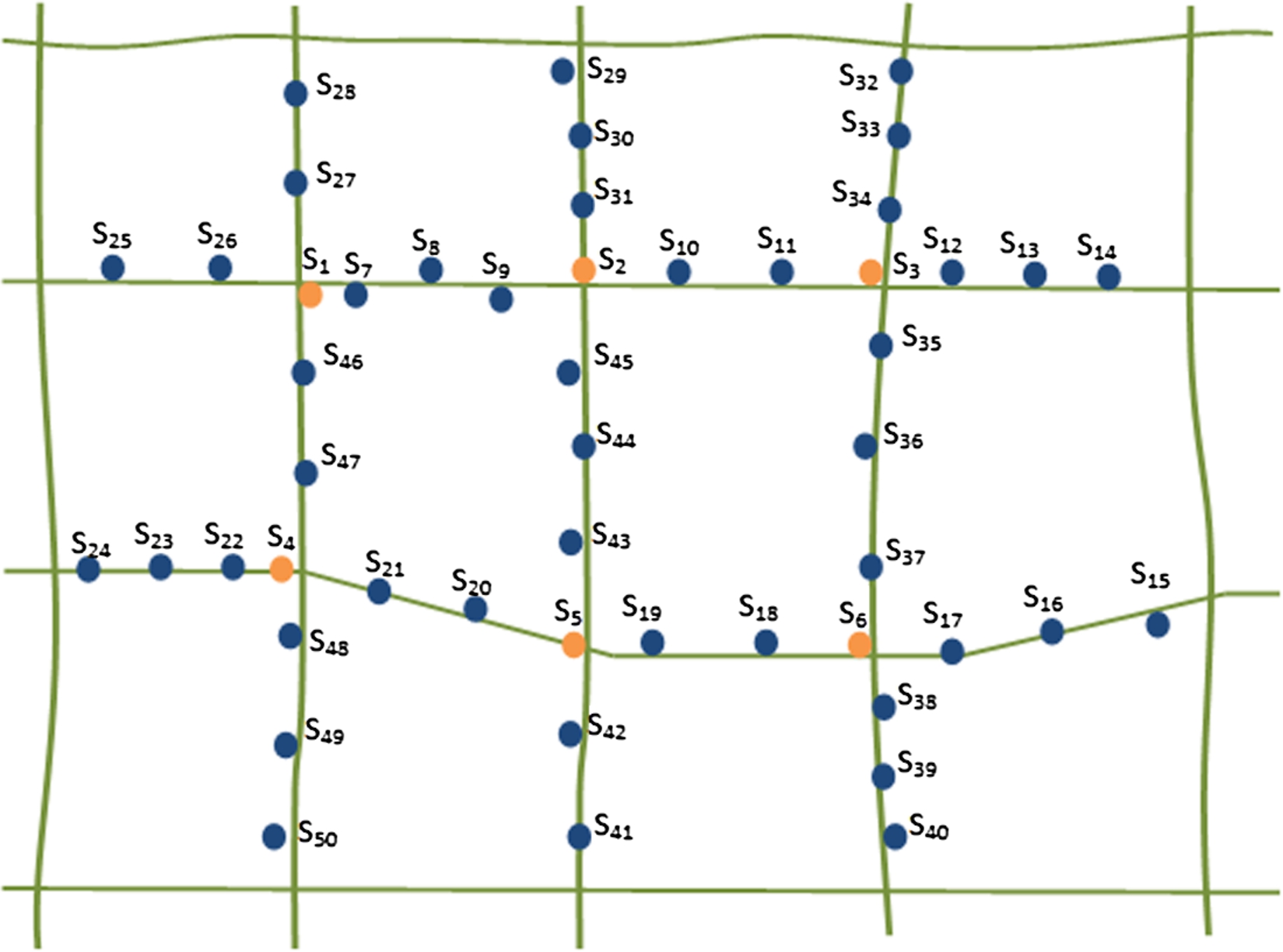
Sensors deployed at an intersection and having more than two neighboring sensors (e.g. Sensors 1–6 in Fig. 3).

Non-intersection nodes:

Sensors deployed at non-intersection points and having a maximum of two neighboring sensors (e.g. Sensors 7–50 in Fig. 3).

Non-intersection node cluster:

Non-intersection nodes in the same road segment which have not yet been ordered.

Non-intersection chain:

Non-intersection nodes within the same road segment which have been ordered (e.g., Sensors 7–9 in Fig. 3).

Endpoint non-intersection nodes:

Nodes at the end of a non-intersection chain (e.g., Sensors 7, 26, 27 and 46 in Fig. 3).

Fig. 3.

Sensors in road network model.

The localization algorithm proposed in this study determines the physical locations of the sensor nodes using only the information provided by the vehicle-detection timestamps. In the proposed approach, each sensor sends its vehicle-detection timestamps and ID to the localization server. The server then analyzes the properties of the vehicular traffic on the basis of the information collected from all the sensors and classifies the sensors into two groups, namely non-intersection node clusters and intersection nodes. The server analyzes the relationship between each pair of sensors in the same non-intersection node chain in accordance with their interarrival time processes and timestamp series; and then constructs an ordered non-intersection chain. In addition, the server estimates the two endpoint non-intersection nodes in each road segment and connects these nodes to the adjacent intersection nodes. By repeating this process for each of the road segments the server gradually constructs a virtual graph of the entire sensor network. Finally, the server maps the virtual graph to the known road map in order to estimate the position of each sensor.

3.2. Road segment classification

In the road segment classification phase, the localization algorithm uses the vehicle detection-timestamp information obtained from the sensors and then classifies the sensors accordingly. In general, every road segment has distinct traffic properties. Thus, sensors in different road segments detect different traffic patterns. Within the same road segment, the information collected by the various sensors exhibits obvious characteristics in the random process. By contrast, different road segments are characterized by distinctly different random properties.

Fig. 4.

The same pattern of TDOD in different road segments.

Fig. 5.

The same pattern of TDOD in same road segment.

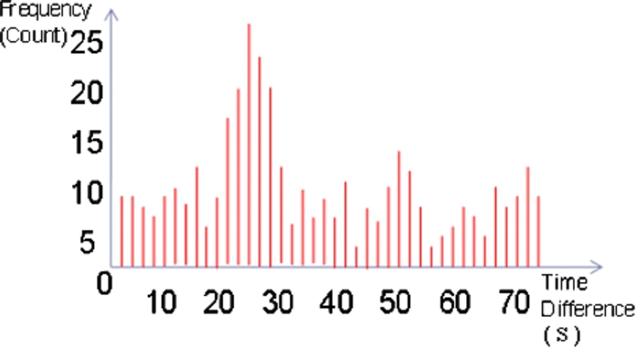
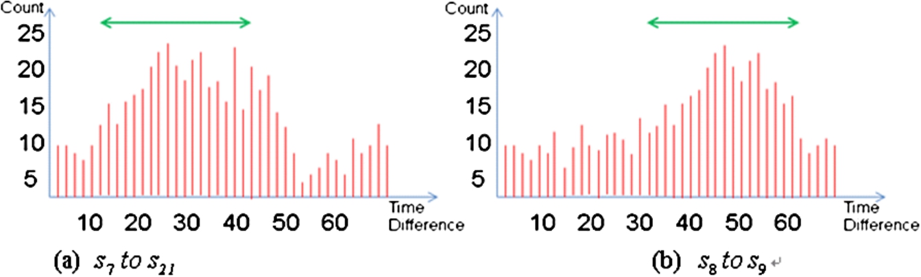
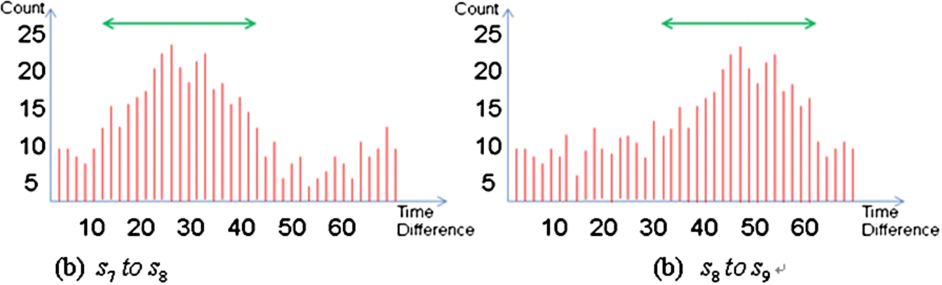
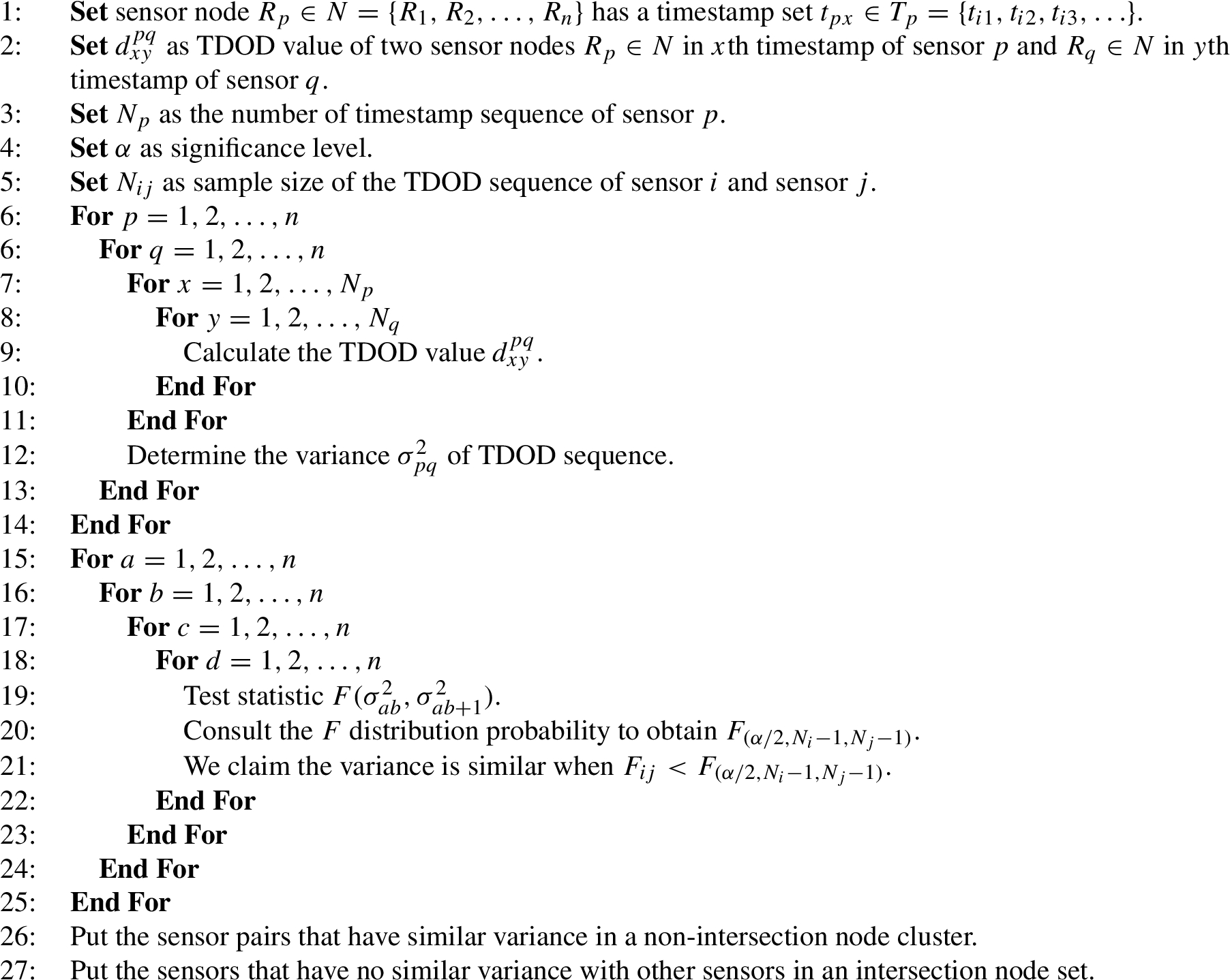
As shown in Figs 4 and 5, the TDOD measurements between two sensors in the same road segment have a strong correlation, while those between two sensors in different road segments have a weak correlation. Therefore, the localization server commences by calculating the TDOD value (i.e., Eq. (1)) for each pair of sensors in the road network, and then performs a statistical test (i.e., F-test) to determine whether or not a statistical difference exists in the TDOD variances of different sensor pairs. Note that the TDOD variance $σ_{i j}^{2}$ between two sensors i and j is formulated as follows: $\begin{matrix} (4) & σ_{i j}^{2} = \frac{1}{N_{i j} - 1} \sum_{k = 1}^{N_{i j}} {(d_{k}^{i j} - μ^{i j})}^{2} \end{matrix}$ where $N_{i j}$ is the sample size of the TDOD sequence corresponding to sensor i and sensor j, $d_{k}^{i j}$ is the kth value of the TDOD sequence corresponding to sensor i and sensor j, and $μ^{i j}$ is the mean value of the TDOD sequence corresponding to sensor i and sensor j. From Eq. (4), the statistical test of these TDOD values can be calculated F-test is formulated as follows: $\begin{matrix} (5) & F (σ_{i j}^{2}, σ_{i k}^{2}) = \frac{σ_{i j}^{2}}{σ_{i k}^{2}}, where i, j, k \in sensors set R = {1, 2, \dots, n} \end{matrix}$

Note that an F-test can be used only if the standard deviations of the two considered populations are equal (i.e., $F (σ_{i j}^{2}, σ_{i k}^{2}) < F_{(α / 2, N_{i} - 1, N_{j} - 1)}$ ). The F-test can be either a one-tailed test or a two-tailed test. A one-tailed test can only determine whether the standard deviation of the first population is larger or smaller than that of the second. Having completed the test, sensor pairs with a similar TDOD variance are assigned to a cluster. Of the nodes which are not assigned to a cluster, some nodes may be intersection nodes. The road segment classification procedure is described in Procedure 1.

Procedure 1:

Road Segment Classification

3.3. Sensor ordering on road segment

The proposed localization algorithm orders the sensors within each non-intersection cluster by comparing the random properties of their interarrival processes and timestamp series. Due to differences in the vehicle speed, rate of acceleration/deceleration, direction of travel, and so forth, the vehicle movements within the network can be modeled as a random process. The interarrival time of the vehicles at each sensor reflects the elapsed time between the passage of two successive cars past the same sensor. For a given road segment, the random properties of the timestamp information generated at each non-intersection sensor are similar to those of the timestamp information generated at its neighboring sensors. Furthermore, the similarity between the random properties of the two sets of timestamp information increases as the distance between the two sensors reduces. For example, if non-intersection sensor A detects a high vehicle density, its neighboring sensor B will also in all probability detect a high vehicle density.

Assume that a total of n sensors exist in the observed road network. Furthermore, assume that the vehicle interarrival times at each sensor form a random sequence. Let m elements be chosen from each random sequence. (Note that a larger value of m can ensure a lower error.) The m elements associated with the n sensors can be evaluated to build n vectors, as shown in Fig. 6.

Fig. 6.

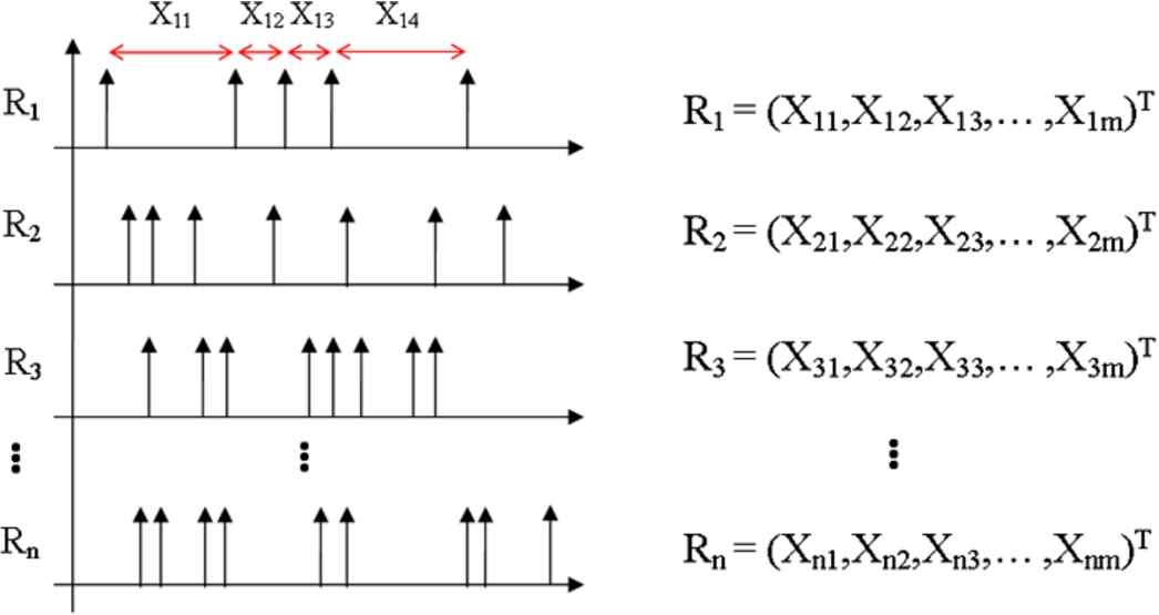
Sensors’ interarrival time.

In the localization algorithm proposed in this study, the means of the random vectors are examined via a two-sample T-test (i.e., Eq. (6)) in order to determine whether or not they are equal. Note that the two means are taken to be equal if the T-test cannot reject the null hypothesis. $\begin{matrix} (6) & T_{i j} = \frac{μ_{i} - μ_{j}}{\sqrt{σ_{i}^{2} / N_{i} + σ_{j}^{2} / N_{j}}} \end{matrix}$ where $μ_{i}$ (or $μ_{j}$ ) is the mean vehicle interarrival time at sensor node i (or j), $σ_{i}^{2}$ (or $σ_{j}^{2}$ ) is the variance of the interarrival time at node i (or j), and $N_{i}$ (or $N_{j}$ ) is the sample size of the interarrival time at sensor node i (or j). The test verifies that the two populations have equal means (i.e., $P (T_{(α / 2, v)} > T_{i j})$ ). Furthermore, in implementing the proposed algorithm, a sufficient number of samples are collected to ensure that the interarrival process approximates a Gaussian distribution and an observed level of significance is obtained. The observed significance levels are then arranged as an ascending power series, and the edges of the ascending power series are connected until all of the sensors in the network are joined. The procedure by which the non-intersection nodes are ordered is described in Procedure 2.

Procedure 2:

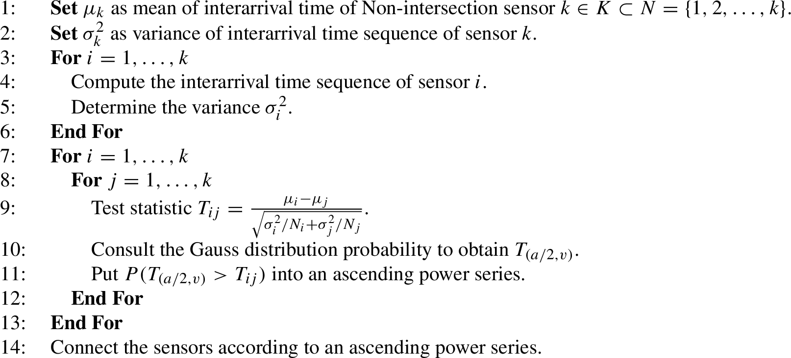
Ordering Non-intersection Nodes (mean)

In addition to the means analysis described above, the covariance of the interarrival time series between two sensors is also examined to test for similarity between the two random processes. The interarrival time series at two neighboring nodes have similar waveforms. Moreover, the degree of similarity between the covariance of the two time series increases as the distance between the two sensors reduces. In the proposed localization algorithm, the random process is partitioned into small intervals (i.e., hourly time windows), and the covariance of the two random processes evaluated accordingly.

Note that by combining the mean and covariance procedures, a greater classification accuracy is obtained.

3.4. Graph construction

In constructing the virtual graph of the sensor network, the localization algorithm searches for all the neighboring sensors of each intersection node in order to localize the node on the corresponding road segment. The non-intersection node chains are then connected to the intersection nodes, thereby forming a virtual graph. Finally, the virtual graph is mapped to the known road map in order to localize the position of each sensor.

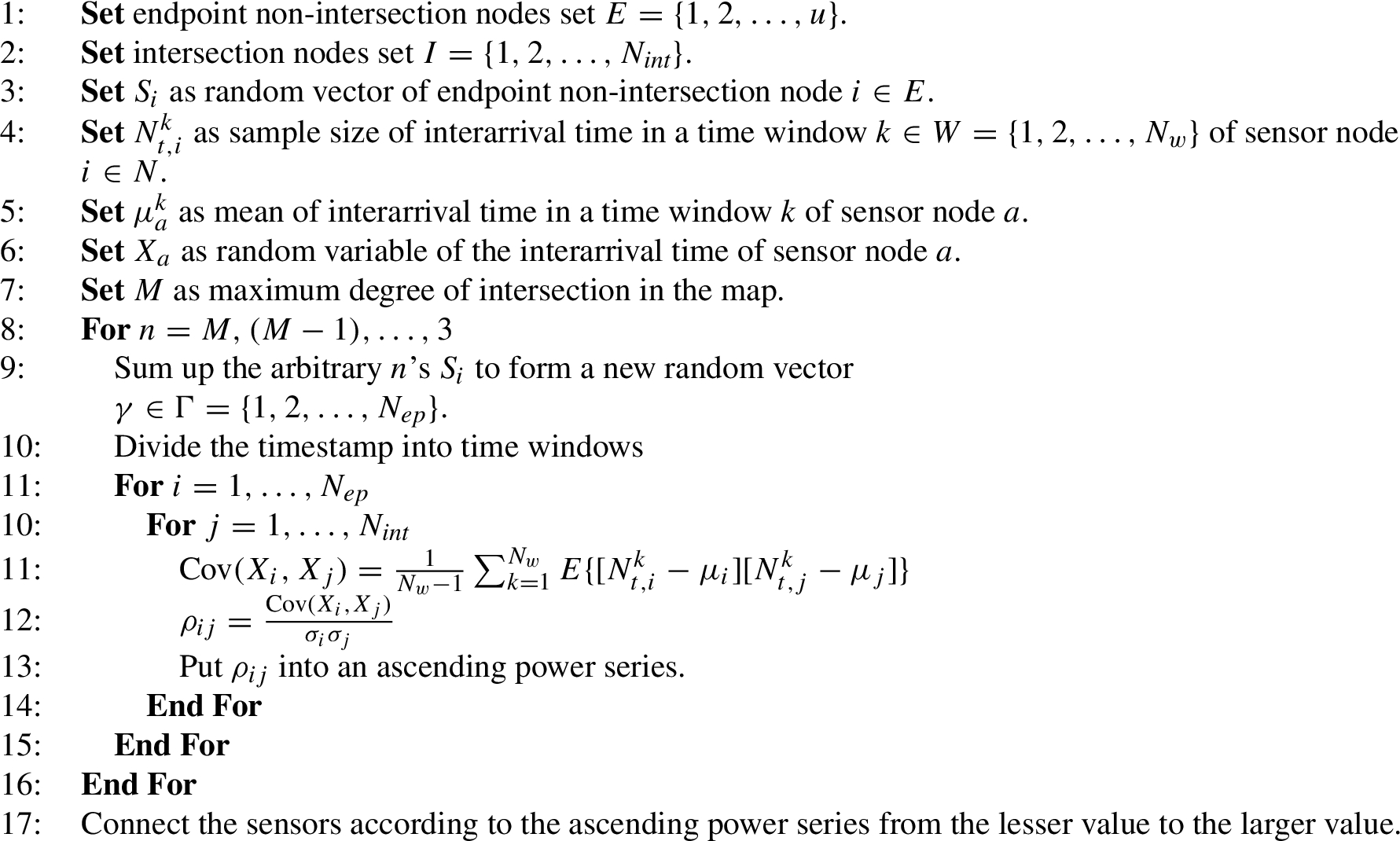
An intersection node receives traffic information from neighboring endpoint non-intersection nodes. As shown in Fig. 7, the interarrival time at an intersection node are related to the interarrival time at the neighboring endpoint non-intersection nodes. Thus, the timestamps of the non-intersection nodes are merged into a new random vector, which is then compared the random vector of the intersection node. By selecting the appropriate non-intersection nodes for comparison with the corresponding intersection node, a high correlation can be obtained.

Fig. 7.

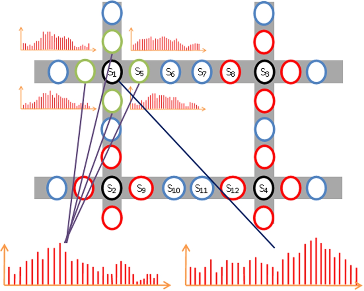
Correlation between intersection and endpoint non-intersection nodes.

Depending on the type of intersections, this algorithm first selects several random vectors corresponding to non-intersection nodes and then sums these vectors to form a new random vector. In practice, the target area may actually contain multiple types of intersection. Therefore, in constructing the virtual graph, the algorithm commences by identifying the different types of intersection within the selected area, and then connects the endpoint non-intersection nodes and intersection nodes in descending order of intersection complexity. For example, suppose that the selected area contains two 5-way intersections, ten 4-way intersections, and one 3-way intersection. The algorithm searches first for five endpoint nodes for each intersection node, and connects the endpoint nodes and the intersection node each time a match is obtained. When no further 5-way intersections can be found, the algorithm searches for four nodes for each intersection node, and constructs the virtual graph accordingly. The process is then repeated to construct the graph for the 3-way intersection.

The new random vector is partitioned into time windows and the number of timestamps in each time window is evaluated. The timestamp numbers are taken as the value of the time windows, and collectively form a random sequence. The localization algorithm then utilizes the same approach to construct a random sequence based on the timestamps generated at the intersection node. Finally, the algorithm determines the covariance (i.e., Eq. (7)) of the two random sequences and normalizes the result to obtain the correlation coefficient shown in Eq. (8). $\begin{array}{l} (7) & Cov (X_{i}, X_{j}) = \frac{1}{N_{w} - 1} \sum_{k = 1}^{N_{w}} E {[N_{t, i}^{k} - μ_{i}] [N_{t, j}^{k} - μ_{j}]} \\ (8) & ρ_{i j} = \frac{Cov (X_{i}, X_{j})}{σ_{i} σ_{j}} \end{array}$ where $μ_{i}$ (or $μ_{j}$ ) is the mean interarrival time at sensor node i (or j), $σ_{i}$ (or $σ_{j}$ ) is the standard deviation of the interarrival time at node i (or j), $N_{t, i}^{k}$ (or $N_{t, j}^{k}$ ) is the sample size of the interarrival time at sensor node i (or j) in time window k, and $N_{w}$ is the total number of windows. A correlation coefficient approaching 1 indicates that the endpoint non-intersection nodes and the intersection node are located in close physical proximity to one another. The procedure for connecting the virtual graph is given in Procedure 3.

Procedure 3:

Connecting Virtual Graph

It is noted that the computational cost of the localization algorithm is dependent on the window size. Specifically, a larger window size results in a greater localization precision, but incurs a greater computational cost. Therefore, a tradeoff must be realized between the precision of the localization process and the computational cost. In the present study, the window size is set to one hour because different hours in the day are often associated with different traffic patterns (e.g., traffic jams in rush hour periods, free-flowing traffic in off-peak hours, and so on). As discussed previously, the level of significance α, i.e., the probability of the null hypothesis is rejected. Specifically, a lower value of α indicates a greater accuracy of the statistical test. In this study, α is assigned the conventional value of 0.05.

4. Simulation results

In this section, the performance of the proposed localization algorithm is compared with that of APL by means of numerical simulations performed on the Opportunistic Network Environment (ONE) simulator [16]. The simulations involved 20 ∼ 120 sensors and 100 vehicles. The vehicles randomly chose their own directions and followed the shortest paths to their destinations. Each road segment was assigned a particular speed limit (maximum speed limit: 65 km/h). The speeds of the vehicles traveling along each segment were uniformly distributed in the interval of (45 km/h, speed limit assigned to road segment). The simulations were performed using the Manhattan street model [2] with a road segment length of 500 m (see Fig. 8). The parameters used in performing the simulations are summarized in Table 1. The error ratio (out of set of predefined sensor locations) which forms the basis of performance evaluation of the simulation is the number of localization error sensors divided by total number of sensors.

Fig. 8.

Simulation road network.

Table 1

Simulation Setup

Parameter	Description
Number of sensors	20–120 deployed
Number of vehicles	100
Vehicle speed distribution	45–65 km/h with uniform distribution
Vehicle arrival period	Each vehicle arrives at road network follow Exponential distribution with mean interarrival time of $1 / λ = 120$ s
Road segment length	500 m
Time synchronization error	Sensor’s time synchronization error conforms to ( $- 0.01$ s, 0.01 s) with uniform distribution

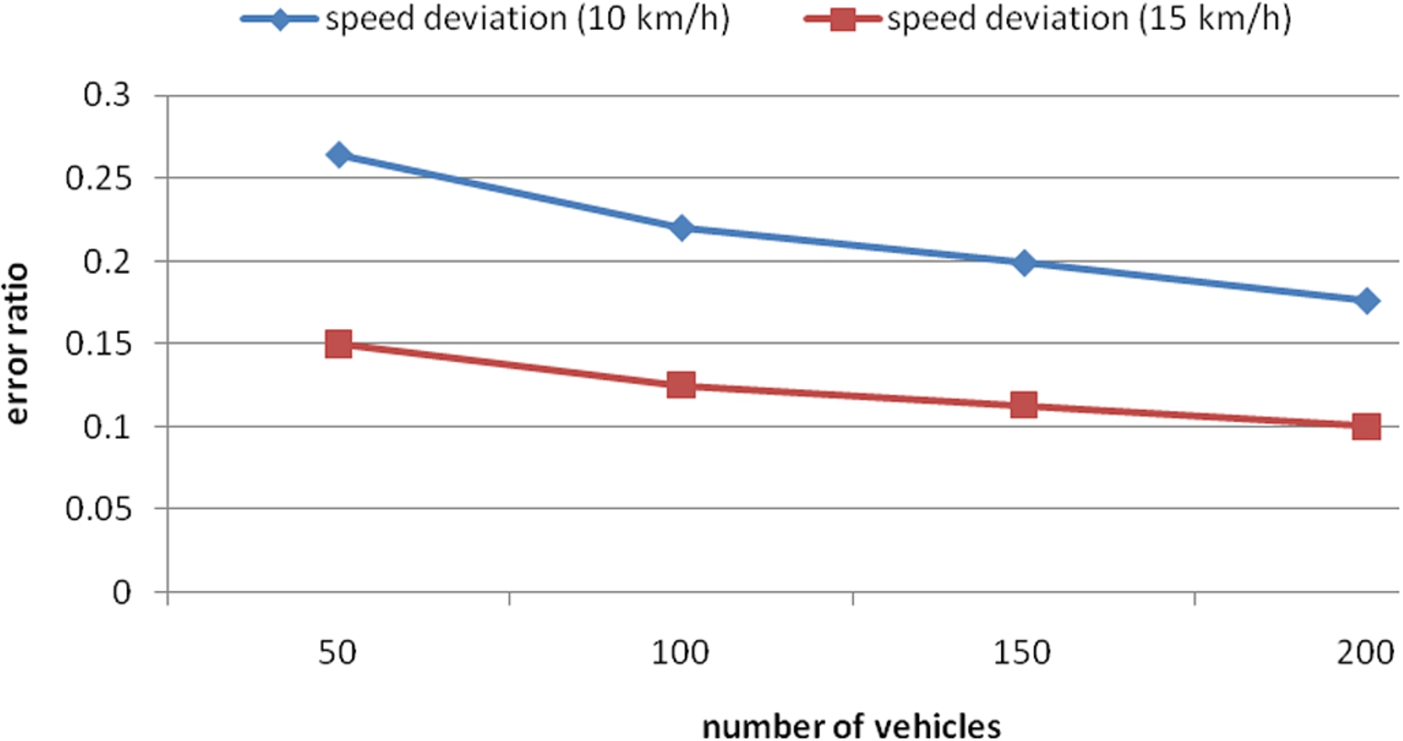
Figure 9 shows the performance of the proposed localization algorithm at given speed deviation (i.e., speed difference). As shown, the error ratio reduces with an increasing speed difference. Since the proposed algorithm is based on binary detection random processes, a high speed deviation results in the acquisition of different detection patterns at sensors located in different positions.

Fig. 9.

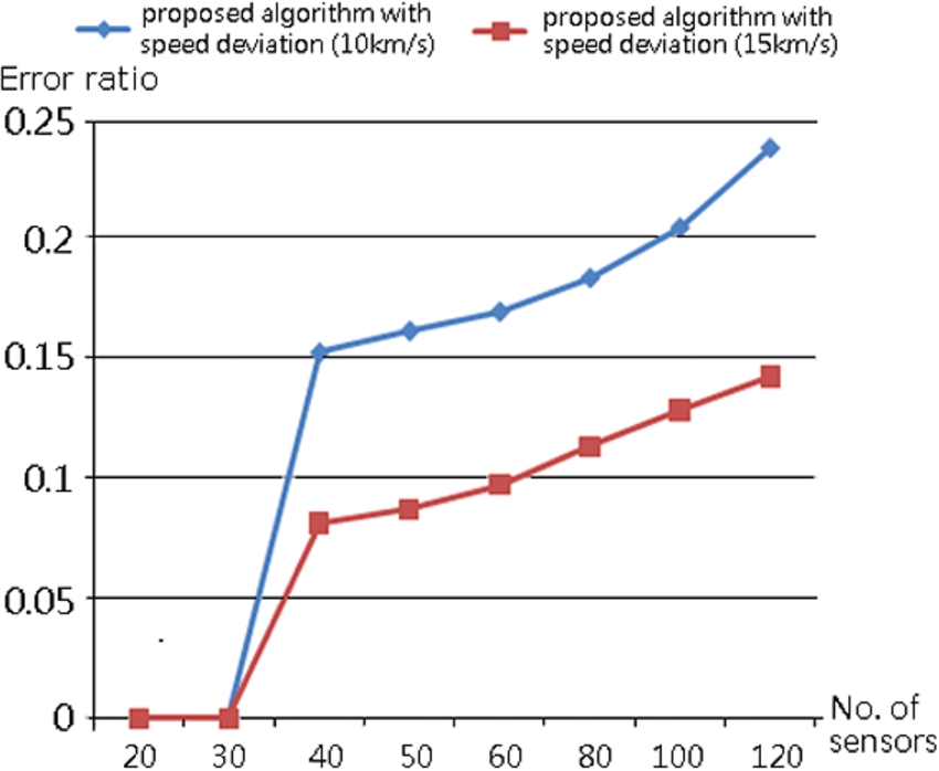
Error ratio on proposed algorithm.

The traffic behavior in an urban environment is more complicated than that in a military environment. That is, the vehicles may randomly stop at some point along a road segment or may suddenly begin to move from a stopped state. Such events add redundant timestamp values (i.e., noise) to the observed timestamp series. Thus, to improve the performance of the localization process, it is necessary to enlarge the sample size (i.e., vehicle detection-timestamp information); thereby reducing the ratio of redundant timestamp information to useful timestamp information.

Fig. 10.

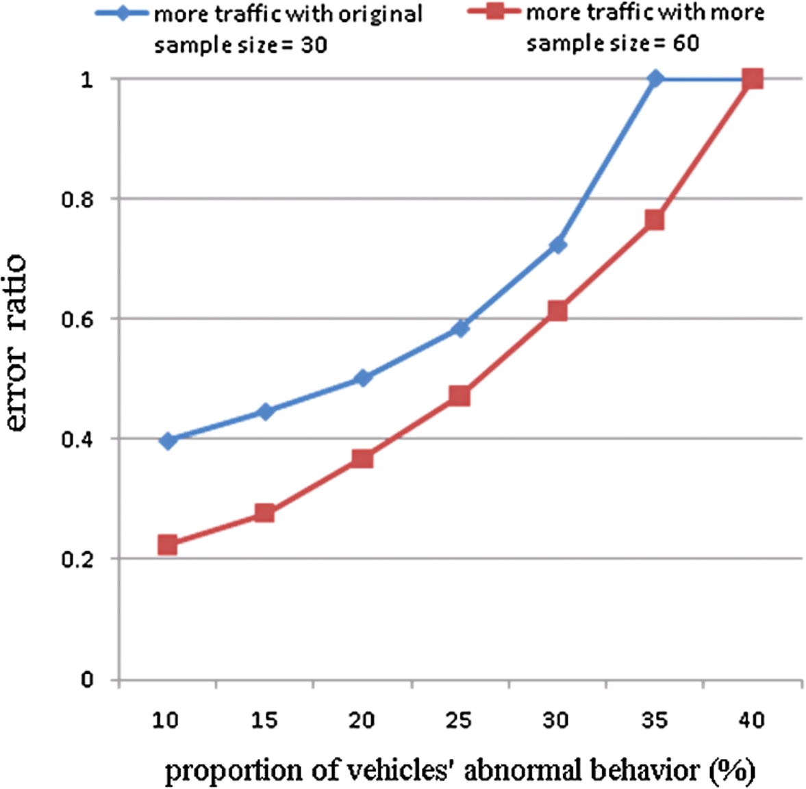
Error ratio with different proportions of noise (vehicles’ abnormall behavior).

Figure 10 shows the performance of the proposed algorithm given different sample sizes for the case where 10–30% of the cars randomly stop and start. It is seen that the error ratio increases exponentially with an increasing amount of noise (i.e., vehicles’ abnormall behavior). However, the localization performance improves with an increasing sample size. Figure 11 shows that the localization error reduces with an increasing vehicle density due to the corresponding increase in the sample size.

Fig. 11.

Error ratio with different vehicle density.

In APL [14], each sensor sends its vehicle-detection timestamps and ID to the server. In other words, the first step of APL is the same as that of the proposed approach. APL then performs a TDOD operation on all of the sensors and estimates the distances between each pair of arbitrary sensors. By contrast, the proposed algorithm finds the similar variance with statistical test through TDOD operation between each pair of arbitrary sensors. In the following step, APL estimates the length of each road segment by evaluating the movement time between the corresponding sensors. The movement time is evaluated by utilizing the correlation between the vehicle-detection timestamp sets of the two sensors subject to the assumption that the mean vehicle speed is approximately equal to the speed limit assigned to the corresponding segment of roadway. As a result, a larger vehicle speed deviation results in a poorer accuracy of the movement time (and hence a poorer precision of the estimated road segment length). On the other hand, in the proposed approach, a high speed deviation results in multiple detection patterns at the sensors located in different positions (see Section 3.2). Therefore, Fig. 12 shows that while APL ceases to function correctly when the speed deviation exceeds a certain value, the accuracy of the proposed algorithm actually improves as the speed deviation increases. There are 200 nodes in this simulation.

Fig. 12.

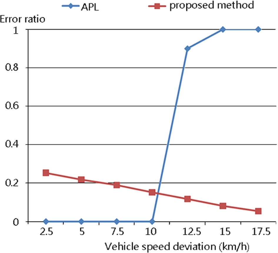
Error ratio of APL and proposed algorithm.

In the proposed algorithm, the variance of the TDOD process is used to classify the non-intersection node clusters and intersection nodes. The accuracy of the classification operation depends on the deviation of the vehicle speed over the road segment. This classification operation can be used to compare the vehicle speed distribution in one road segment with that in another. If the vehicle speed deviation is very small, the difference between the two distributions is not sufficiently distinct. Thus, the tendency of the error ratio for the algorithm proposed is this study is the reverse of that for APL.

In final scenario, it contains two 5-way intersections, eleven 4-way intersections, and seven 3-way intersection in selected area. Figure 13 shows that the proposed algorithm retains a localization ability in a network environment with heterogeneous intersection types. In addition, it exhibits a lower error ratio than that in a homogenous environment containing 4-way intersections only because the intersections in different types have distinct traffic properties. The lower error ratio arises as the result of a misclassification of some of the intersection types within the simulation environment.

Fig. 13.

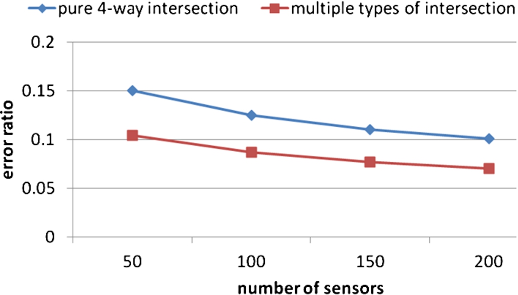
Error ratio in multiple types of intersection.

5. Discussion

The following additional scenarios should also be mentioned:

(1) Large-scale networks: In large-scale networks (i.e., networks containing a very large number of intersection nodes), the performance of the proposed localization algorithm may be degraded. However, a large target area can be regarded as the combination of several smaller areas (i.e., fewer intersections). The localization accuracy would be improved by dividing the road network into several smaller areas with localization performed by a different server in each area.

(2) This section concludes with a comparison of the computational complexities of APL and the proposed algorithm, respectively. As discussed above, APL performs a TDOD operation in the first step. The TDOD operation is performed $C_{2}^{n} = (n^{2} - n) / 2$ times, where n is the number of sensors. In other words, the complexity is $O (n^{2})$ . In the second step, APL performs the minimum spanning tree and the relative deviation error with complexities of $O (E + vlogv)$ and $O (n^{2})$ , respectively. Thus, the total complexity of APL is $O (n^{2})$ . The algorithm proposed in this study also performs TDOD in the first step. However, in this case, the algorithm iterates through all TDOD variances in order to identify the non-intersection nodes. Consequently, the first step has a complexity of $O (n^{4})$ . In the second step, the algorithm computes the mean of the interarrival time and the covariance of the time series with complexity $O (n^{2})$ . In the final step, the endpoint non-intersection nodes are combined with the intersection nodes with a complexity of $O (n^{2})$ . In other words, the total complexity of the proposed algorithm is greater than that of APL. However, the algorithm outperforms APL even when the assumption of a uniform vehicle speed is relaxed.

6. Conclusion

This study has proposed an algorithm for localizing the roadside sensors in a traffic network using only binary detection information. The proposed localization approach is based on the covariance and means properties of the sampled binary detection random processes and is accomplished using simple, low-cost sensors. It has been shown that by classifying the sensors as intersection nodes or non-intersection nodes, a good localization performance is obtained under both high speed deviation conditions and noise conditions. Furthermore, it has been shown that for a similar level of computational complexity, the proposed algorithm provides a better localization performance than the APL scheme, even when the assumption of a uniform vehicle speed on each road segment is relaxed. In the future, this study will extend its related issues, e.g. issues in larger dense networks, and compare our extended study with more localization algorithms.

Footnotes

Acknowledgement

This work was supported in part by National Science Council under the Grant NSC 98-2219-E-006-010.

References

Aghajarian and

Berangi, A fast distributed target tracking algorithm for low density binary sensor networks, in: Second International Conference on Sensor Technologies and Applications, 2008, pp. 1–6.

Bai,

Sadagopan and

Helmy, IMPORTANT: A framework to systematically analyze the impact of mobility on performance of routing protocol for ad hoc network, INFOCOM 2 (2003), 825–835.

Bulusu,

Heidemann and

Estrin, GPS-less low cost outdoor localization for very small devices, IEEE Personal Communications Magazine 7(5) (2000), 28–34. doi:10.1109/98.878533.

W.Y.

Chiu,

B.S.

Chen and

C.Y.

Yang, Robust relative location estimation in wireless sensor networks with inexact position problems, IEEE Trans. Mobile Comput. 11(6) (2012), 935–946. doi:10.1109/TMC.2011.111.

Corke,

Hrabar and

Peterson, Autonomous deployment and repair of a sensor network using an unmanned aerial vehicle, 2004 IEEE International Conference on Robotics and Automation (2004), 3602–3608. doi:10.1109/ROBOT.2004.1308811.

Cucuringu,

Lipman and

Singer, Sensor network localization by eigenvector synchronization over the Euclidean group, ACM Trans. Sensor Netw. 8(3) (2012), 19. doi:10.1145/2240092.2240093.

R.W.

Deming and

L.I.

Perlovsky, Concurrent multi-target localization, data association, and navigation for a swarm of flying sensors, Information Fusion 8(3) (2007), 316–330. doi:10.1016/j.inffus.2005.11.001.

Elkin,

Kumarasiri,

D.B.

Rawat and

Devabhaktuni, Localization in wireless sensor networks: A dempster-Shafer evidence theoretical approach, ad hoc networks 54 (2017), 30–41. doi:10.1016/j.adhoc.2016.09.020.

Fang,

Nan,

Jiang and

Chen, Robust node position estimation algorithms for wireless sensor networks based on improved adaptive Kalman filters, Computer Communications 101 (2017), 69–81. doi:10.1016/j.comcom.2016.11.005.

10.

Gu,

Jia and

Vicaire, Lightweight detection and classification for wireless sensor networks in realistic environments, in: Proceedings of the 3rd International Conference on Embedded Networked Sensor Systems, 2005, pp. 205–217. doi:10.1145/1098918.1098941.

11.

Guo,

K.S.

Low and

M.J.

Er, Probability field localization algorithm for wireless sensor network, in: 32nd Annual Conference on IEEE Industrial Electronics, 2006, pp. 3155–3160.

12.

Guo,

K.S.

Low,

Nguyen and

M.J.

Er, Localization in a Sparse Wireless Sensor Network Using Pedometer and Communication Ranging Measurements, IEEE Industrial Electronics Society, IECON (2007).

13.

He,

Huang,

B.M.

Blum,

J.A.

Stankovic and

Abdelzaher, Range-free localization schemes for large scale sensor networks, in: Proceedings of the 9th ACM Annual International Conference on Mobile Computing and Networking, 2003, pp. 81–95.

14.

Jeong,

Guo,

He and

Du, APL: Automous passive localization for wireless sensors deployed in road networks, in: 27th Conference on Computer Communications, 2008, pp. 583–591.

15.

Kanji, 100 Statistical Tests, 3rd edn, SAGE, London, 2006.

16.

Keranen,

Tot and

Karkkainen, The ONE Simulator for DTN Protocol Evaluation, 2nd international conference on simulation tools and techniques, 2009.

17.

Lazos and

Poovendran, SeRLoc: Secure range-independent localization for wireless sensor networks, in: Proceedings of the 2004 ACM Workshop on Ireless Security, 2004, pp. 21–30. doi:10.1145/1023646.1023650.

18.

Liu,

Zhang and

Bu, A locality-based range-free localization algorithm for anisotropic wireless sensor networks, Telecommun. Syst. 62(1) (2016), 3–13. doi:10.1007/s11235-015-9978-8.

19.

Moore,

Leonard,

Rus and

Teller, Robust distributed network localization with noise range measurements, in: SENSYS, ACM, 2004, pp. 50–61.

20.

Niculescu and

Nath, Ad Hoc Positioning System (APS) using AoA, in: Proceedings of IEEE International Conference on Computer Communication, 2003, pp. 1734–1743.

21.

Niculescu and

Nath, Error characteristics of Ad Hoc Positioning Systems (APS), in: Proceedings of the 5th ACM International Symposium on Mobile Ad Hoc Networking and Computing, 2004, pp. 20–30.

22.

Ollero,

Bernard and

La Civita, AWARE: Platform for autonomous self-deploying and operation of wireless sensor-actuator networks cooperating with unmanned aerial vehicles, in: Proc. IEEE Int. Workshop Saf., Secur. Rescue Robot, SSRR, 2007, pp. 1–6.

23.

Patwari,

A.O.

HeroIII and

Perkins, Relative location estimation in wireless sensor networks, IEEE Trans. on Signal Processing Special Issue on Signal Processing in Networking 51(8) (2003), 2137–2148.

24.

N.B.

Priyantha,

Balakrishnan and

Demaine, Anchor-free distributed localization in sensor networks, in: Proceedings of the 1st International Conference on Embedded Networked Sensor Systems, 2003, pp. 340–341. doi:10.1145/958491.958550.

25.

N.B.

Priyantha,

Chakraborty and

Balakrishnan, The cricket location-support system, in: Proceedings of the 6th ACM Annual International Conference on Mobile Computing and Networking, 2000, pp. 32–43.

26.

Romer, The lighthouse location system for smart dust, in: Proc. of 1st ACM International Conference on Mobile Systems, Applications, and Services, 2003, pp. 15–30.

27.

Savvides,

C.C.

Han and

M.B.

Srivastava, Dynamic fine-grained localization in ad-hoc networks of sensors, in: Proceedings of the 7th ACM Annual International Conference on Mobile Computing and Networking, 2001, pp. 166–179.

28.

Shen,

Ding,

Dasgupta and

Zhao, Multiple source localization in wireless sensor networks on time of arrival measurement, IEEE Trans. Signal Process. 62(8) (2014), 1938–1949.

29.

Sichitiu and

Ramadurai, Localization of wireless sensor networks with a mobile beacon, in: Proc. Int. Conf. on Mobile Ad-Hoc and Sensor Systems, 2004, pp. 174–183.

30.

Stanoev,

Filiposka,

In and

Kocarev, Cooperative method for wireless sensor network localization, ad hoc networks 40 (2016), 61–72. doi:10.1016/j.adhoc.2016.01.003.

31.

Stoleru,

He and

J.A.

Stankovic, A high-accuracy, low-cost localization system for wireless sensor networks, in: Proceedings of ACM Conference on Embedded Networked Sensor Systems (SenSys), 2005, pp. 13–26.

32.

Stoleru,

Vicaire,

He and

J.A.

Stankovic, StarDust: A flexible architecture for passive localization, in: Wireless Sensor Networks, In Proceedings of ACM Conference on Embedded Networked Sensor Systems, 2006, pp. 57–70.

33.

Xiao,

Bu,

Wang and

Xiao, Robust localization against outliers in wireless sensor networks, ACM Trans. Sensor Netw. 9(2) (2013), 24.

34.

Yao and

Jiang, Distributed wireless sensor network localization based on weighted search, Comput. Netw. 86 (2015), 57–75. doi:10.1016/j.comnet.2015.05.002.

35.

Zeliang and

Lihua, Mobile anchor nodes aided DV-hop (M-A-DV-hop) algorithm, in: International Workshop on Education Technology and Training & 2008 International Workshop on Geoscience and Remote Sensing, 2008, 2008, pp. 312–315.

36.

Zhang,

Liu,

Wang,

Cao and

Min, Accurate range-free localization for anisotropic wireless sensor networks, ACM Trans. Sensor Netw. 11(3) (2015), 51.

37.

Zhao,

Xi,

He,

Liu,

X.Y.

Li,

Mo and

Yang, Localization of wireless sensor networks in the wild: Pursuit of ranging quality, IEEE/ACM Trans. Netw. 21(1) (2013), 311–323. doi:10.1109/TNET.2012.2200906.

38.

Zhong and

He, MSP: Multi-sequence positioning of wireless sensor nodes, in: Proc. 5th Int’l Conference Conf. Embedded Networked Sensor Systems, 2007, pp. 15–28. doi:10.1145/1322263.1322266.