
Abstract
Nowadays, mobile users are equipped with multi-mode terminals allowing them to connect to different radio access technologies like WLAN, 3G (HSPA and HSPA+), and Long term evolution (LTE) each at a time. In this context, the challenge of the next-generation networks is to achieve the Always Best Connected (ABC) concept. To this end, solving the problem of selecting the most suitable radio access technology (RAT) from the list of available RAT is at the heart of the next-generation systems. The decision process is called access network selection and it depends on several parameters, such as quality of service, mobility, cost of each RAT, energy consumption, battery life, etc. Several methods and approaches have been proposed to solve the network selection problem with the fundamental objective which is to offer the best QoS to the users and to maximize the usability of the networks without affecting the users’ experience. In this paper, we propose an adaptive KNN (K nearest neighbour) based algorithm to solve the network selection problem, the proposed solution has a low computation complexity with a high level of veracity is compared with the well-known MADM methods.
Introduction
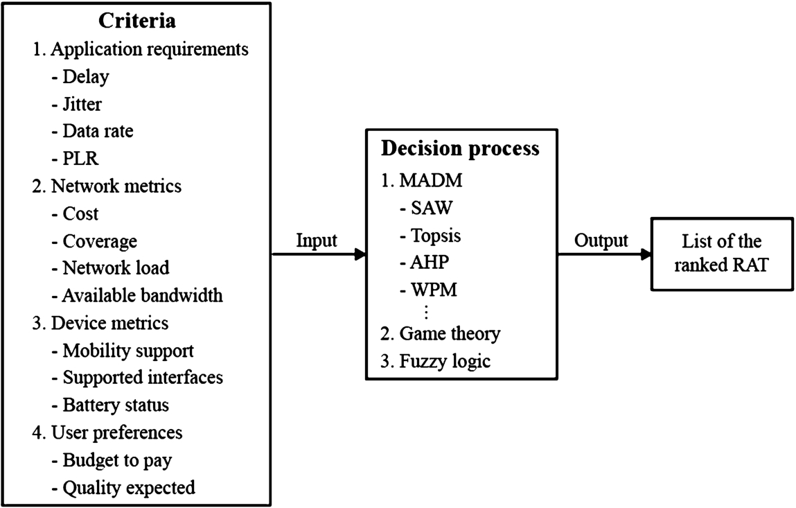
The next generation of wireless networks is characterized by the coexistence of various wireless access technologies such as the famous WLAN precisely IEEE802.11, and the cellular networks such as, UMTS, HSPA, and LTE. Its aim is to achieve the ABC concept by offering mobile users the ability to take advantage (basically, to look for the best QoS possible) of the available RATs with different architectures and performances. This variety and differences constitutes the elements of the heterogeneous environment [10]. In a heterogeneous environment Fig. 1, users are enabled to choose a RAT among a list of available RATs based on several criteria, this choice is called the network selection procedure and this is the scope of this paper [9].
The network selection procedure consists in the selection of the best available network among those accessible [10]. The term “best network” differs from one user to another due to the various preferences involved in the process like cost, energy consumed, mobility…, but, all users agree on the seek for the best QoS [16,36]. The network selection procedure is modelled as Multiple Attribute Decision-Making (MADM) methods. Indeed, MADM approaches have been widely used to solve the network selection problem [8,15,36]. Other methods like fuzzy logic and game theory [16,34,38] have also been used for the same end. Many studies in the literature propose algorithms that select a network among a set of candidate. Other relevant methods pertaining to multi-criteria optimization have been used to deal with the NS problem as well. These include artificial intelligence, neural networks, and genetic algorithms. For us, in this paper, we are proposing to adapt a machine learning algorithm named K- nearest neighbour (KNN) [12] to solve the network selection problem. The KNN algorithm is known by its ease and low complexity to classify the competitors. So, we will take advantages of these qualities, and we will adapt it for our problem.
The rest of this paper is organized as follows. Section 2 is dedicated to related work, we will give works that treated the NS problem by telling their pros and cons. In Section 3, we will present the KNN algorithm and the way we adapt it to solve the NS problem; in this section, we will present the results obtained, and we will discuss them. Finally, the paper ends with a conclusion and perspectives.

Heterogeneous wireless environment.
Several works in the literature treated the network selection problem, these works focus mainly on offering users a high-quality experience in order to support many services with the best possible QoS in a smoother manner. In the following, we present an overview of the related works in the field of network selection.
In [28] the authors have used the Simple Additive Method SAW to get a ranked list of networks, while in [27] the authors made a mix between game theory and the SAW method.
The main benefits of the SAW method are the simplicity and low computation complexity; meanwhile, it has two major drawbacks:
A parameter can be outweighed by another one. The rank reversal phenomenon is still a big problem of the entire MADM approach.
In [2] the authors have proposed an algorithm based on TOPSIS, the weight vector is calculated using the Entropy formula. They claim that the obtained results prove that the proposed algorithm selects the best available network in heterogeneous environments based on user preferences and service requirements.
A comparative study between SAW and WPM in the context of vertical handover is performed [29]. The authors used the relative standard deviation as a metric of comparison, and they conclude that WPM is better than SAW. In [20], the authors used the M-ANP method in the context of heterogeneous systems, their conclusion is that the combination of M-ANP with TOPSIS is a robust method to make dynamic decisions and to avoid neglecting and underestimating attributes with poor quality. In [22], AHP method is used to rank the importance of different criteria and to compare the pertinent of different Internet advertising networks; the proposed model provides an objective and effective decision model for advertisers to be used in selecting an Internet advertising network. Authors in [31] have proposed a Fuzzy AHP method and compared it with the original version of AHP, the comparison is based on the Quality of Experience QoE; indeed, the authors used the fuzzy complementary matrix and the fuzzy consistent matrix to relax the consistency requirements in AHP. The Numerical results show that the proposed scheme Fuzzy AHP outperforms the conventional AHP scheme.
The MADM methods are widely used to solve the network selection problem, this is due to the multiple criteria nature of the network selection problem. In addition, these methods are easy to use and understand, they have also a relatively-low computational complexity.
The drawbacks of these methods are summarized as follows:
The MADM methods have not the same performance toward the different services (VoIP, Video Calls, web browsing), indeed, generally, these methods have a high performance for the VoIP service, although they have a bad performance for the best-effort services. These differences involve great problems because users utilize always different services. MADM methods suffer from the problem of ranking abnormality, which is a phenomenon occurring in the MDAM methods when an replica or a copy of an alternative is introduced or omitted, authors in [37] have shown that the rank reversal problem occurs in most of the well-known MADM methods, this problem has been addressed in other works [18,32] by modifying methods, but the original versions of MADM methods suffer from this phenomenon. Another remark to add is that some methods including AHP are very complicated and have a high complexity of computation.
For these reasons, we can say that MADMs are a good option and acceptable solution for the network selection problem, but they must be modified to take care of their drawbacks especially the rank reversal phenomenon which is a big problem.
It is worth mentioning that in the literature, there is no work using KNN algorithm in the context of network selection. So, we can assert that our work is the first which uses KNN to solve the network selection problem. We also have not used KNN in its original version, we adapt it to be usable in our case study. In the following section, more details are found.
Problem context and formulation
In this section, we will give details on the network selection problem, the mathematical model of this problem, we will also present the KNN algorithm and how we adapt it to use it in our case.
Network selection description
The network selection process consists of the intelligent and automatic switching between different available RATs [6,7], to be always best served. So, when a multimode user discovers the existence of various RATs within its area, it should be able to select the best network in terms of delay, jitter, throughput, and packet loss rate (Fig. 2).
The process of selecting the best RAT depends on plenty of parameters: battery level, the energy required to get the requested services, the RSS received, cost, the bandwidth acquired, the user preferences, QoS required, etc. These parameters are categorized into four groups [10]
Network conditions parameters: It includes information about network conditions: network load coverage area, network connection time, available bandwidth, Application requirements parameters: the information about the threshold needed by the service application to be in the normal state, as well as the required throughput, delay, jitter, packet loss rate, and energy needed for the application, User preference parameters: information relative to end-users, i.e. user acceptable cost, preference between cost and service quality, Mobile equipment parameters: information about the user’s device, i.e. battery level status, and mobility [11].
The network selection procedure is started when a new service is requested, such as a video/VoIP call or a data transfer service, also when the received RSS drops below the threshold value and after the user’s radio connection worsens, for instance when the user is mobile. As far as the application requirements are concerned, NS depends on the type of service desired. For VoIP, delay and packet loss rate are the important parameters, while for the video calls service, the important criteria are the bandwidth and the latency of the packets, whilst for the best effort service, the data rate offered is the one who we care about the most.
Network selection process.
As a mathematical description of the network selection we used [13] During the network selection procedure, we consider multiple attributes together, so the utilities of multiple attributes are combined as a total utility. It has been pointed out in [36] that a valid form to combine these attributes together satisfies the following requirements.
In this subsection, we describe the well-known methods used to solve the network selection. In particular, MADM methods, these methods are used in Section 4 to make the comparison with our proposal.
Simple additive weight SAW
SAW is a well-known method for the case of multiple criteria systems, it assumes that the treated data had the same unit. So, to get a comparable scale among parameters, it is mandatory to normalize the data for each parameter [1,27,28]. Finally, the candidate having the highest/lowest value is selected.
The mathematical formulation of SAW is:
Generally, SAW method has been widely used in the context of network selection, [25,27,28]. In [28] and [25] authors have used the SAW method to get a ranked list of networks, while in [27] authors have made a mix between game theory and SAW method. When authors treat the NS problem using SAW method and other variance, the main benefit of the SAW method resides in its simplicity and low complexity, however its drawback is that one parameter can be outweighed by another one.
Technique for order preference by similarity to ideal solution TOPSIS
TOPSIS is an aggregating compensatory method based on the concept that the chosen solution should have the shortest geometric distance from the positive ideal solution [26] and the longest geometric distance from the negative ideal solution. The normalized data for each parameter is weighted, and therefore the geometric distance between each alternative and the ideal alternative is computed. The TOPSIS process is carried out as follows:
Create an evaluation matrix consisting of m alternatives and n criteria, with the intersection of each alternative and criteria given as, The matrix Calculate the weighted normalized decision matrix where
Determine the best and worst alternative Calculate the separation measure each alternative
Calculate the relative closeness to the ideal solution
TOPSIS has been applied in the network selection problem in several works, such as [4,28,30]. In [28], authors compare the performance of vertical handover HO using SAW and TOPSIS, they concluded that TOPSIS outperforms the SAW method. In general, we can say that compensatory methods, namely TOPSIS managed to avoid the problem that a parameter can be outperformed by another one by allowing a trade-off between criteria. This means that a poor value in one criterion can be neglected by a good value in another criterion. This provides a huge power and gets more sense than non-compensatory methods, which use thresholds system.
Weighted product model WPM
WPM called also Multiplicative Exponential Weighting MEW is similar to SAW [21]. The difference is the replacement of the addition operation in the SAW method with the multiplication operation in the WPM method; each decision alternative is compared with the other ones by multiplying a number of ratios, one for each decision criterion. Each ratio is raised to the power equivalent to the relative weight of the corresponding criterion. The mathematical description is as follows:
Authors in [29] have made a comparison between the SAW and WPM methods in the context of vertical handover, they use the relative standard deviation as a metric of comparison, and they obtain a conclusion that WPM is better than SAW method. In [33], authors use the WPM method in the context of heterogeneous systems, their conclusion is that the WPM method is a more robust approach for the dynamic decision-making, and it penalizes the attributes with poor quality.
Analytical hierarchy process AHP and grey relational analysis GRA
AHP considers decomposition of one complicated problem to a multiple hierarchy of simple sub-problems [35]. The AHP steps are as follows:
Decompose the problem to a hierarchy of sub problems, where the top node is the final goal and for each criterion, we list the alternatives. Pair-wise comparison of attributes and translating them into numerical values from 1 to 9. Calculates the weights of each level of hierarchy. Synthesizing weights and getting overall weights. Normalization of data is performed considering three situations: the higher is better through the lower is better, and nominal is the desired. Definition of the ideal sequence in the three considered situations: the ideal sequence contains the higher bound, lower bound and moderate bound. Computing the grey relational coefficient (GRC): the more favourable sequence is when the GRC is larger.
Regarding GRA method, it is used to rank the candidate networks, and it regroups the following steps:
The AHP method is usually coupled with Grey relational Analysis GRA method, the AHP for weighting and the GRA is used to rank alternatives.
Other MADM methods have been used for the network selection problem, like VIKOR [24], SWARM [23], ELECTRE [3]…, others approaches that are not a MADM methods, like fuzzy logic, genetic algorithms, game theory, utility functions…, these methods and approaches were not considered (in the comparison with our proposal) in this paper for many reasons:
Some of them are complicated with a high computation complexity and at the end, they give a similar performance like the methods that we presented. This is not a survey or a review paper, so we cannot present all methods used for making the network selection procedure
It is important to mention that these methods are applicable only when all data of the input matrix are expressed with the use of the same unit. Therefore, data must be normalized, which is an important step in the network selection procedure. Different normalization methods exist in the literature like, the max-min method that is used in this paper, the sum method, the square root method and others.
Adaptive KNN algorithm
In this section, our contribution will presented in details.
KNN algorithm
K-Nearest Neighbour [12] is one of the simplest Machine Learning algorithms based on Supervised Learning technique [19]. KNN algorithm assumes the similarity between the new case/data and available cases and put the new case into the category that is most similar to the available categories. KNN algorithm stores all the available data and classifies a new data point based on the similarity. This means when new data appears, then it can be easily classified into a well suite category by using KNN algorithm. KNN algorithm can be used for regression as well as for classification, but mostly it is used for the classification problems. Generally, KNN algorithm is used to classify things, i.e. the result is kind of “this item belongs to class x”. In our case, we have adapted this algorithm to give us a ranking order of the different RATs.
The original KNN algorithm can be explained on the basis of the below steps:
Adaptive KNN algorithm
So, our idea is to fix a vector with the ideal values of QoS to have a high-quality experience of any service without any interruption. These values (for throughput, latency, jitter, and Packet loss rate PLR) are extracted from literature and older works, high-level papers based on experiences and simulations, for example, (
It is well-known and obvious that lower values for latency, jitter, and PLR are good for the user instead of higher values. For the throughput, a higher value is what we seek, in our minimizing system, so we use the inverse of the value (maximizing a value is equivalent to minimize its inverse) to be fair with the other criteria of the system, which must be minimized. The inverse value is either the negative value of the original one or using the original value with the exponent minus one. The two uses are quite similar, in fact, the derivative of the two functions
So after preparing our data, for each QoS criterion, a higher Euclidean distance between each QoS value of the vector of ideal values and the offered QoS measures of each RAT means a lower value for the criterion and this is what we need.
We also adapt the KNN algorithm by modifying the meaning of the “K”, indeed, the K was used to fix the number of neighbours of the data in each class and assigns the new data points to that class for which the number of the neighbours is the highest. In our case, the “K” is used to rank the RATs, a smaller K (
The “Adaptive Knn algorithm” steps are as follows:
Weight vector based on Eigenvector method Generate instant QoS values for each RAT Fix the vector of ideal QoS values
The proposed Adaptive KNN algorithm is depicted in the following Algorithm 1.
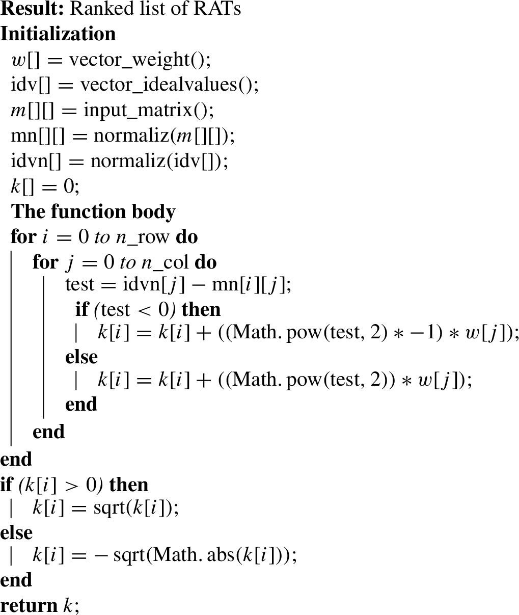
Adaptive KNN algorithm
So we start by making initializations, then we calculate distance between vector of ideal QoS values and the QoS vector of each RAT, at the end, the ranking is performed based on the vector of distances. Large distance means that the RAT is far away from the vector of ideal QoS values, so this RAT is not appropriate for the user, in the contrary, the RAT is best suited for the suer.
In this section, a performance evaluation of the proposed approach is performed, the performance of our algorithm is tested with different types of service namely (VoIP, video service and best effort applications).
The services are represented by the vector weight, it means that each service has its QoS parameters which are more important than others, for example, for the VoIP service, the throughput is not so important because of the small packet of voice service, but, the latency, the jitter and the PLR are so important. So, for this service, the weight vector will give higher value for latency, jitter and PLR and lesser one for throughput. For Video calls service, the throughput is important duo to the large packets (voice and image), the latency, the jitter and PLR are also so important so for this service, almost all the QoS parameters are equally important. For the best effort service, the throughput is the important one, with the PLR [5]. The values of the weight vector are calculated using the eigenvector method, this method is widely used to get weight values, for instance, it is used also by the AHP method. SO, we use it in our study because later, we will do a comparison with MADM method among them AHP method, so to be fair, we are using the same method of weight. The weight vector is presented in Table 1 [5].
Based on Algorithm 1, our proposal needs 3 inputs, the weight vector (we already have it in Table 1), we need the instant value for RATs, and we also need to fix the ideal vector of suited values for each QoS parameter. The range values of these parameters are presented in Table 2, the values are generated from simulations. Also, we need to fix the vector of ideal values for each RAT, the values of this vector are extracted from literature where authors did experiences to fix these values and also from the RATs standards (IEEE for WiFi and 3GPP for HSPA and LTE) [14,17]. The values are described in Table 3.
So, we have defined all our inputs (the vector of ideal values, the weight vector and the range values of QoS). Now, we need to generate QoS values for each RAT to be used in our simulations Table 4; these values are generated randomly based on Table 2. Three types of simulations (VoIP, video calls and best effort) are performed to test the performance of our proposal and compare it with the legacy MADM methods (SAW, TOPSIS, WPM and AHP-GRA).
The weight vector
The weight vector
QoS parameter’s range values
QoS parameter’s ideal values
The input matrix for the simulation
We start our simulation and comparison using the values of Table 4 and simulating them for the case of VoIP service. In this case, the delay, jitter and PLR are the most important QoS parameters (see Table 3). We compare our proposal with the well-known MADM methods (SAW, TOPSIS, WPM and AHP) the results are presented in Table 5.
VoIP ranking results
VoIP ranking results
Table 5 gives the ranking results in the case of VoIP service. Each algorithm gives its ranking for the data given by Table 4, Table 3 and Table 1. Now, we will make a comparison to see which algorithm is more accurate.
QoS comparison L1 vs W1 for VoIP.
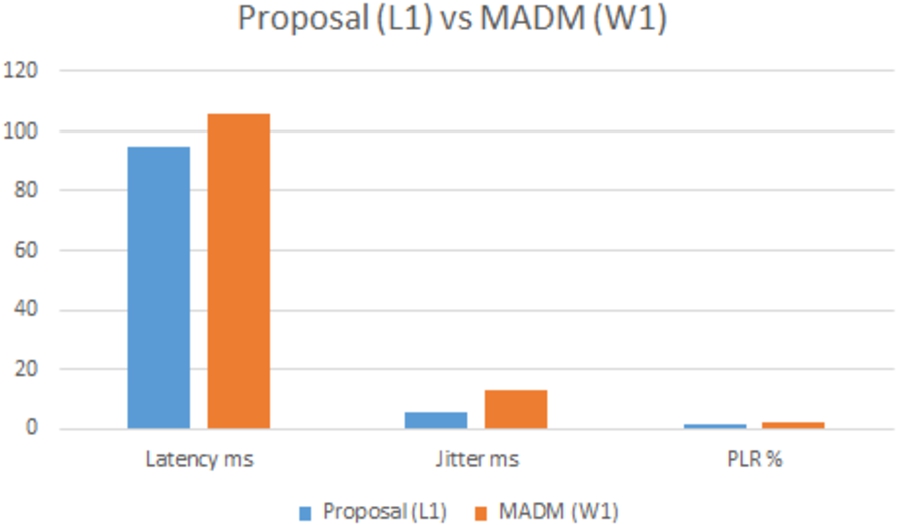
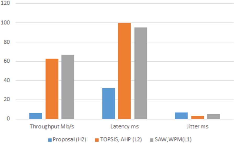
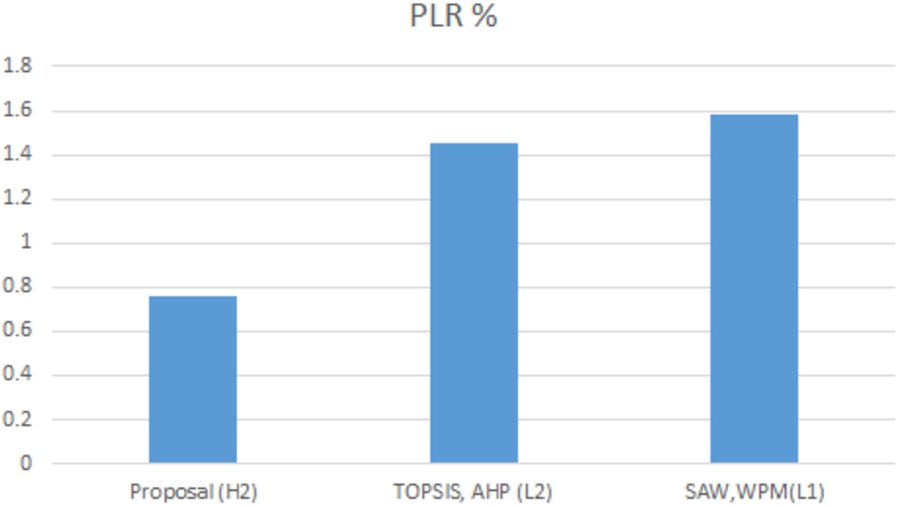
The first remark on Table 5 is that the MADM methods and our proposal rank “H2” with the first place (i,e. H2 is the best choice), “H1” is ranked the second for all methods. However, in the third place our proposal says that “L1” is more suited, but MADM methods claim that “W1” is the adequate. So, we will compare these two networks (L1 and W1) for each parameter and see. “L1” has the following QoS values (Throughput 66.66 Mbs, latency 95.15 ms, jitter: 5.31 ms and 1.58% PLR), meanwhile “W1” has (Throughput 1.73 Mbs, latency 105.85 ms, jitter: 13.13 ms and 1.98% PLR). It is clear that “L1” is more suited compared to “W1” see image 3.
Figure 3 confirms our purposes and shows that “L1” is more suited than “W1” and the MADM methods have performed a wrong ranking compared to our proposal.
The second simulation concerns the video service. So, based on Table 4, Table 3 and Table 1, the video service are sensitive to throughput, PLR, jitter and latency respectively with different coefficients, see Table 1. The results of the experience are presented in Table 6.
Table 6 represents the comparison between the different methods (MADM methods and our proposal), it shows that SAW and WPM methods ranks “L1” with first choice, TOPSIS selects “L2”, AHP, chooses “H1” and for our proposal, “H2” is taken. The Figs 4 and 5 gives a comparison between these networks. Figure 4 is for comparing latency and jitter between the different methods for their first ranking choice. It is clear that for latency the choice of our proposal is the optimum, even for jitter. Figure 5 represents the comparison in terms of PLR, the proposal is suited and gives adequate packet loss rate.
Video service ranking results
Video service ranking results

Jitter, latency and PLR comparison for video service.
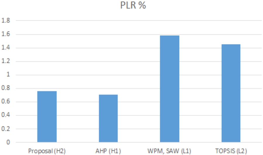
PLR comparison for video service.
Finally, we simulate the methods for the best effort service, such as web browsing and file downloading. The results are presented in Table 7.
Figures 6 and 7 show that for latency and PLR, our chosen network is the best one with less than half of the values presented by the other networks selected by the other methods, for jitter, the networks in competition present similar values. For the throughput, the other networks “L1 and L2” certainly have excellent, but also “H2” has a value above the required one so it fits our necessary throughput.
Best effort service ranking results
Best effort service ranking results
Our work address another issue for the MADMs which is the rank reversal problem. Indeed, In decision-making, a rank reversal is a change in the rank ordering of alternative possible decisions when, for example, the method of choosing changes or the set of other available alternatives changes. The issue of rank reversals lies at the heart of many debates in decision-making and multi-criteria decision-making, in particular. So, we will test our proposal with the legacy MADM methods and see which methods are sensitive to rank reversal and those that are not.
Jitter and latency comparison for best effort service.
PLR comparison for best effort service.
So, in our case, delete one RAT which is “L1” and run the algorithms (MADM methods and our proposal) and see the ranking order.
Simulation of rank reversal case
Results in Table 8 show that, all the MADM (TOPSIS, SAW, WPM and AHP) methods suffer from the rank reversal problem because the ranking results presented in Table 8 are different from those shown in Table 5. This result confirms the affirmation of the authors in [37] that all MADM methods suffer from the rank reversal problem.
We can see also that our proposal does not present the rank reversal phenomenon when a network disappears; indeed, our proposed method just removes the disappeared alternative while keeping the other alternatives rank unchanged. This is an excellent result for our approach.
This paper represents a case study and a proposed solution of the network selection problem. An adaptive Knn based algorithm is presented, and the performance are evaluated for different types of services (VoIP, video services and best effort ones). The comparison with the legacy MADM (SAW, TOPSIS, WPM and AHP) shows that our proposal outperforms these latter. We perform another comparison for the rank reversal phenomenon, which is a well-known problem of the MADM. Our proposal eliminates this situation, and it is not affected by the disappearance of a given RAT. The lack of our proposal, the mobility aspect of users is not well modelled and expressed.
As we started using artificial intelligence in network selection, we consider implementing a basic neural network to make the choice for users instantly and automatically without any interaction of this latter based on the RAT conditions and user behaviour.
Conflict of interest
The author has no conflict of interest to report.