A prioritized decision making method for reliability allocation: In optimistic and pessimistic view

Abstract

Reliability allocation is a very important problem during early design and development phases of a system. There are several reliability allocation techniques which are used to achieve the target reliability. The feasibility of objectives (FOO) technique is one of them that is widely used to perform system reliability allocation. But this technique has two fundamental shortcomings. The first is the measurement scale and the second is that it does not consider the order weight of the reliability allocation factors. The prioritization of the factors is also an important topic in decision making. Practically, all factors in multi-criteria decision making (MCDM) are not in the same priority level. Hence, in decision making situation, it is usual for decision makers to consider different priority factors. So, considering the prioritization of the factors, a reliability allocation method is proposed here to overcome the shortcomings of the FOO technique. Also, a case study on reliability allocation in airborne radar system is considered here to verify the efficiency of the proposed approach. Finally, the results are calculated in different optimistic and pessimistic view point and compared with the FOO technique. This comparison exhibits the advantages and supremacy of the proposed approach.

Keywords

Reliability allocation/apportionment FOO technique prioritized decision making

1 Introduction

Reliability allocation is a fundamental task during the manufacturing stages of any engineering system. The main aim is to allocate the target reliability to the subsystems and guarantee that the system can achieve its target goals (Bona et al. (2018), Ronchieri and Canaparo (2018), Covino et al. (2000)). In reliability allocation, the allotment of the resources significantly influences the quality of the product and system’s operational success. Therefore, an effective reliability allocation method is required to allocate the reliability to the system.

In the year of 1957, Advisory Group on Reliability of Electronic Equipment (AGREE, 1957) proposed a reliability allocation method depending upon the subsystem’s criticality and complexity rather than failure rate. After that in 1964, considering the failure rate of subsystems, Aeronautical Radio Inc. published the ARNIC method (William & Alven, 1964). In the same year, Brcha (Bracha, 1964) proposed another allocation technique considering the factors: state-of-the-art, complexity, environmental condition and operating time. Whereas, in 1965, Karmiol introduced the apportionment technique based on complexity, criticality, state-of-the-art and operational time. More recently, another important technique namely feasibility of objectives (FOO) technique has been published in the Mil-hdbk-338B handbook (United States Department of Defence, 1988) for military reliability design. There are also some reliability allocation methods like average weighting allocation (Kuo, 1999), integrated factor method (Felice et al., 2010), improved agree method (Liang et al., 2018) etc. But all have a common fault in the scale of measurement. In these methods discrete ordinal scales are used to measure the ratings of the factors which mislead the results. Also the system factors are not similarly weighted which creates some problems to make a decision.

To rectify these problems (Chang et al., 2009) developed some methods based on the Yager’s OWA operator. (Chen. et al., 2015) also proposed a reliability allocation technique considering uncertain preferences which can also overcome the previous problems.

In reality, when a decision is made, all criteria do not get equal importance. Considering this fact, the importance of different criteria is regarded as the priority of criteria. Practically in MCDM situation, it is habitual for decision makers to think about various priorities of criteria. In the literature, many studies have been done including various priorities of criteria in MCDM problems. Yager (2004) proposed that the prioritization of criteria can be modelled by using importance weights. Here he established that the weights associated with the lower priority criteria are interconnected to the satisfaction of the higher priority criteria. In further extension, Yager (2008) introduced a prioritized averaging/scoring aggregation operator using product T-norm. Thereafter, several researchers (Chen and Wang (2009), Yan et al. (2011)) also focused on MCDM problems considering multiple priorities.

In this study, a maximal entropy minimal variance Ordered weight averaging (MEMV-OWA) operator based prioritized reliability allocation method is proposed considering multiple priorities in criteria. Using this operator an attempt has been made to minimize the variance of weighting vector and to maximize the entropy. Moreover, our proposed method can overcome the drawbacks of the previous reliability allocation methods.

The remaining portion of the article is arranged as follows: Section 2 creates a survey on reliability allocation method and its drawbacks. Section 3 presents some theoretical background on the ordered weight averaging operator and its properties. Section 4 introduces the concept of prioritization of criteria and also discusses about OWA operator with priorities. Based on this concept, in Section 5, a prioritized reliability allocation method is proposed. A numerical example has been solved in Section 6 to establish the flexibility of the proposed approach. Also, a comparison with FOO technique and a discussion under different optimistic and pessimistic view point are given in the same section. Finally, Section 7 provides a conclusion on the overall work.

2 Reliability Allocation Methods

Reliability allocation/apportionment is a critical procedure to allocate the target reliability into each subsystem considering trade-off among multiple attributes ((Hu et al. (2019); Yu et al. (2018)). It is highly required to apportion a feasible reliability to every subsystem. There are different reliability allocation techniques like ARNIC (1964), AGREE (1957), the FOO technique (MIL-HDBK-338B, 1988), the average weighted allocation method (Kuo, 1999) etc. Among these techniques, FOO technique has enormous uses for reliability allocation. The general concept, procedure and shortcomings of FOO technique are discussed below.

2.1 FOO technique ((MIL-HDBK-338B, 1988); (Chang et al., 2009))

FOO technique was initially proposed as a procedure of apportioning reliability to the non-repairable mechanical-electrical components. In this technique allocation factors are system intricacy, state-of-art, performance time and environmental conditions. The numerical ratings of these factors are assessed by the experts based on their past experience. Each rating is on a 1 to 10 scaling system, with values allotted as given below:

System intricacy (I):

The system intricacy has a strong effect on the reliability of the system. Generally, the failure rate of highly intricate system is going to be high. So the allocated failure rate is proportional to the complexity of the subsystem. Thus the subsystem with higher complexities should be allocated lower reliability targets.

The least intricate system is allotted as a value of 1 and extremely intricate system is allotted as a value of 10.

State-of-art (S):

The least developed design is set as 10, and the extremely developed design is set as 1.

Performance time (P):

The component that works for the whole completion time is assigned as 10 and the subsystem that works the minimal time amid the completion time is assigned as 1.

Environment (E):

Environmental conditions are likewise evaluated from 10 to 1. Components anticipated that would encounter cruel and extremely serious situations are assigned as 10, and those normal to experience the least serious situations are assigned as 1.

The ratings are given by the design experts depending upon their knowledge and experience. The overall ratings are obtained by multiplying the four ratings for every subsystem. i.e, ISPE= I × S × P × E. Where system intricacy, state of art, performance time and environment factors are denoted by I, S, P and E respectively.

Let a system is formed by N subsystems. Suppose λ _s be the system failure rate,λ _k be the allocated failure rate to k^th subsystem, C _k′ denotes the complexity of element k, and R _k′ be the composite rating for subsystem k. R′ is the summation of the composite ratings and r _ik′ denotes the i^th rating for each factor of subsystem k, ∀i ∈ (I, S, P, E). R _s is the target reliability and T is the overall completion time. Then the basic equations of FOO technique (MIL-HDBK-338B, 1988) are: $λ_{s} = \sum λ_{k}$ (1) $λ_{k} = {C_{k}}^{'} λ_{s}, \forall k$ (2) ${C_{k}}^{'} = \frac{{R_{k}}^{'}}{R^{'}}, \forall k$ (3) ${R_{k}}^{'} = {r_{Ik}}^{'} \times {r_{Sk}}^{'} \times {r_{Pk}}^{'} \times {r_{Ek}}^{'}$ (4) $R^{'} = \sum_{k = 1}^{N} {R_{k}}^{'}$ (5)

Drawbacks of FOO techniques (Chang et al., 2009):

The FOO technique has a vast application in reliability allocation. However, this technique has been censured for two crucial deficiencies. The first deficiency is that the four factors (I, S, P and E) are assessed by discrete ordinal measurement scale. As ISPE value is evaluated by the product of the ratings of I, S, P and E, so multiplication is meaningless. The second deficiency is that the factors are not similarly weighted, consequently making problems to analyse and understand the outcomes. For instance, let two component with ISPE value of 9 × 2 ××2 × 2=72 and 7 × 3 ×2 × 2=84 respectively, the previous should allocate a higher reliability than the later. But in practice, as the previous ISPE value is less than the later, the FOO technique allocates lower reliability to the previous. Hence, I, S, P and E are not similarly weighted with respect to each other.

3 Theoretical background

3.1 Ordered weight averaging operator (OWA operator)

The OWA operator was first introduced by Yager (1988) which is an important aggregation operator.

Definition 1. OWA operator (Chen et al., 2015)

An n-dimentional OWA operator is a mapping F: Rⁿ → R, with an associated weight vector W = (w ₁, w ₂, . . . . . . , w _n) ^T such that ∑w _i = 1, ∀ w _i ∈ [0, 1] , i = 1, 2, . . . . , n . with the properties, $f (a_{1}, a_{2}, . . . . ., a_{n}) = \sum_{i = 1}^{n} w_{i} b_{i}$ (6) where b _i is the i^th largest element in the vector (a ₁, a ₂, . . . . . , a _n) and b ₁ ≤ b ₂ ≤ . . . . . ≤ b _n

Definition 2. Measure of Orness (Chen et al., 2015)

Let F is an OWA operator with a weight function W= (w ₁, w ₂, . . . . . , w _n). The degree of orness associated with the weight vector of the operator is defined as: $orness (W) = \frac{1}{n - 1} \sum_{i = 1}^{n} (n - i)$ (7) where orness(W)∈[0,1] is denoted by α, which is a situation parameter.

α= 1 describes the situation when the decision maker is maximally optimistic(a pure optimistic)and α = 0.5 is considered when the decision maker faces a moderate assessment.

Definition 3. Measure of Entropy ((Chen et al., 2015), (Liaw et al., 2011))

The measure of entropy is the degree of utilization of information in an uncertain environment. This is also known as the measure of dispersion and is defined by $disp (W) = - \sum_{i = 1}^{n} w_{i} {lnw}_{i}$ (8)

The properties include:

When w _i = 1 the dispersion of W is minimum, and disp(W)=0.(∵∑w _i = 1) This denotes that only one criteria is taken in the aggregation process.

When w _i= $\frac{1}{n}$ , i=1,....,n, the dispersion of W is maximum and disp(W)=ln(n). This denotes that all criteria are taken in the aggregation process.

Definition 4. Measure of Variance (Chen et al., 2015)

The measure of variance deduces the variability of weight vector for a given level of orness and is explained as $D^{2} (W) = \frac{1}{n} \sum_{i = 1}^{n} [w_{i} - E (w)]^{2} = \frac{1}{n} \sum_{i = 1}^{n} {w_{i}}^{2} - {(\frac{1}{n} \sum_{i = 1}^{n} w_{i})}^{2} = \frac{1}{n} \sum_{i = 1}^{n} {w_{i}}^{2} - \frac{1}{n^{2}}$ (9)

Basically, measure of variance helps to avoid overestimating of a single attribute and control the variance of weighting vector in the decision-making process including multiple criteria.

3.2 Maximum entropy-minimum variance ordered weight averaging operator (MEMV-OWA)

Depending upon the concept of entropy and variance of OWA operator, a bi-objective model can be formulated to obtain the weighting vector of the MEMV-OWA operator (Chen et al., 2015). Here entropy is maximized to utilize the uncertain information of the decision maker’s experience and variance of the weighting vector is minimized to avoid overestimation of the decision maker’s preferences. So, the model is:

$\begin{matrix} Maximize : & - \sum_{i = 1}^{n} w_{i} {lnw}_{i} \\ Minimize : & \frac{1}{n} \sum_{i = 1}^{n} {w_{i}}^{2} - \frac{1}{n^{2}} \\ Subject to : \sum_{i = 1}^{n} & \frac{n - i}{n - 1} w_{i} = α, (0 \leq α \leq 1) \\ \sum_{i = 1}^{n} w_{i} = 1, 0 \leq & w_{i} \leq 1, i = 1, 2, . . . ., n . \end{matrix}$ (10) where, w _i denotes weight of the i^th criteria, n denotes number of attributes, α denotes situation parameter.

For solving this model, weighted sum method is used here to transform the bi-objective problem into a single objective model giving equal weights to both the objectives. Then LINGO software is used for final solution.

3.3 Triangular norms (Yan et al., 2011)

A T-norm is a function T : [0, 1] × [0, 1] → [0, 1] which has the following properties:

Commutativity: T(x,y)= T(y,x)

Monotonicity: T (x, y) ≤ T (u, v)if x ≤ u and y ≤ v

Associativity: T(x,T(y,u))=T(T(x,y),u)

The number 1 acts as identity element: T(x,1)= x

And typical example of T-norms are:

Minimum t-norm: T _min (x, y) = min (x, y)

Product t-norm: T _prod (x, y) = x . y(the ordinary product of real numbers)

Lukasiewicz T-norm: T _Luk (x, y) = max (0, x + y - 1)

4 Prioritization of criteria (Yan et al., 2011)

Suppose a set of criteria C are divided into Q distinct priority levels, H = (H ₁, . . . . . . , H _q, . . . . , H _Q) when H _q = (C _q1, . . . . . . . , C _qk, . . . . . , C _{qN
_q}),N _q is the number of criteria in priority level H _q. C _qk is the k^th criterion of the priority level H _q. Then the prioritization of the priority level is considered as H ₁ > . . . . . . > H _q > . . . . . . . . > H _Q . Total set of criteria is $C = \cup_{q = 1}^{Q} H_{q}$ . For each criterion C _qk, a value C _qk (.), is considered indicating degree of satisfaction of a given alternative with respect to criterion C _qk.

Table 1
Priority hierarchy of a set of criteria C

Priority level Criteria

H ₁ C ₁₁ ... C _1k ... C _1N

.... ... ... ... .... ...

H _q C _q1 ... C _qk ... C _{qN
_q}

..... .... .... ... ... ...

H _Q C _Q1 ... C _Qk ... C _{QN
_Q}

Priority level			Criteria
H ₁	C ₁₁	...	C _1k	...	C _1N
....	...	...	...	....	...
H _q	C _q1	...	C _qk	...	C _{qN _q}
.....	....	....	...	...	...
H _Q	C _Q1	...	C _Qk	...	C _{QN _Q}

Yager categorized this hierarchy into two cases:

Strict priority order Every priority level contains only one criterion, i.e. N _q=1 for q=1,.....,Q.

Weakly order prioritization If any priority level contains more than one criterion, then that prioritization is defined as weakly order prioritization.

4.1 Prioritized weighted aggregation operator (Yan et al., 2011)

The OWA operator has some interesting properties like symmetry, monotonicity, idempotence and compensativeness. Owing to these properties, this operator can be considered to calculate degree of satisfaction for each priority level. Considering decision maker’s situation parameter α toward priority level H _q according to MEMV-OWA weight determination method(eq: 10), each priority level H _q can be related with an weighting vector such that W _q = (w _q1, w _q2, . . . . . . , w _qk, . . . . . , w _{qN
_q}) where w _qk ∈ [0, 1] and $\sum_{k = 1}^{N_{q}} w_{qk} = 1$ . Also let B _q (.) = (b _q1 (.) , b _q2 (.) , . . . . . . . , b _{qN
_q} (.)) be the reordered vector of C _q (.) = (C _q1 (.) , . . . . . . . . . . , C _{qN
_q} (.)) where b _qk (.) is the k^th the largest in priority level H _q. Then the degree of satisfaction in H _q is ${Sat}_{q} (.) = {OWA}_{α_{q}} [H_{q}] = \sum_{k = 1}^{N_{q}} b_{qk} (.) w_{qk}$ (11)

According to Yager (2004), the criteria with lower priority will become significant when the degree of satisfaction of higher priority level has been achieved. Motivated by this perception, each priority level is connected with a priority weight Z _q (.), which is obtained from all the higher priority level’s degree of satisfaction. Moreover, T-norms is unable to remunerate the low values by high values, so T-norms are utilized to incorporate the priority weight Z _q (.) at each priority level.

Particularly, for priority level H ₁, the priority weight Z ₁ (.) =1; for H ₂, Z ₂ (.) = T (Z ₁ (.) , Sat ₁ (.)); for H ₃, Z ₃ (.) = T (Z ₂ (.) , Sat ₂ (.)). Thus the priority weight for H _q is given as: $Z_{q} (.) = T (Z_{q - 1} (.), {Sat}_{q - 1} (.)) = T_{l = 0}^{q - 1} {Sat}_{l} (.)$ (12) with Z ₀ (.) = Sat ₀ (.) =1

So, in this way a priority weight Z _q (.) for priority level H _q can be calculated. Moreover in priority level H _q, there is a local OWA weight with respect to each criteria. In the same priority level to maintain the trade-off between criteria, we should see the degree of satisfaction of each priority level as a pseudo criterion. Along these ways, the aggregated value under the prioritized criteria for each alternative can be calculated as

$V (.) = \sum_{q = 1}^{Q} Z_{q} (.) {Sat}_{q} (.)$ (13)

5 Proposed prioritized reliability allocation method

The basic steps are:

Step 1: Make a list of subsystems that constitute the system.

Step 2: Decide the system’s target reliability and overall completion time.

Step 3: Define the scale for each criteria. The values are considered as a numerical rating.

Step 4: Formulate a matrix considering the numerical ratings and then normalize it.

Step 5: Determine the priority level of the criterion.

Step 6: Compute the degrees of satisfaction of subsystems at each priority level and evaluate the overall rating V (k) for the k^th subsystem using equation 13.

Step 7: Calculate the complexity C _k′ for k^th subsystem ∀k using the formula ${C_{k}}^{'} = \frac{V (k)}{\sum V (k)}$ .

Step 8: Evaluate the system failure rate based on the equation $λ_{s} = - \frac{\ln (R_{s})}{T}$ , where R _s and T are the target reliability and overall completion time of the system respectively.

Step 9: Assess the allocated failure rate for each subsystem using equation 2.

Step 10: Calculate the overall ratings and the reliability allocation values at different α.

Step 11: Analyse the overall results and allocate the optimal reliability to the different subsystems.

6 Case study

To check the applicability of the proposed approach, an example of an airborne radar system (Chen & Wang, 2009) is considered here. It is a detection system that uses radio waves to determine the range, angle or velocity of objects. It can be used to detect aircraft, spacecraft, guided missiles and weather formations. This system is composed of five major line reducible units (LRUs), ancillary installation materials and an equipment rack. The LRUs are composed of antenna (ANT), radar data computer (RDC), radar target data processor (RTDP), transmitter (TRAN) and Filter. In this system, Transmitter (TRAN) produces electromagnetic waves in the radio or microwaves domain and an antenna (ANT) is used for transmitting and receiving the signal. Then the FILTER helps for modulation and filtering of signals and finally the processor (RTDP) to determine properties of the objects. Also RDC (Radar Data Computer) is one of the main sub-systems of airborne radar, responsible for radar operations such as radar control, pre-processing, target detection, tracking and post processing. The design of the airborne radar system is shown in Fig. 1.

Fig. 1

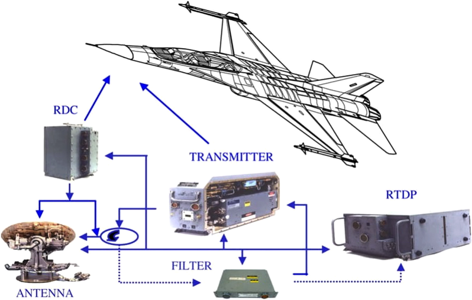
General structure of the airborne radar system.

Depending upon the experts decision, the system reliability target is set as 0.9971429 and the completion time is 2.4h. In this paper I, S, P, E are considered as the reliability allocation factors and the priority level of the criteria’s are set as [H ₁ = I] > [H ₂ = S] > [H ₃ = P, E].

6.1 Results

Solutions based on FOO technique: FOO technique uses the I, S, P and E (ISPE value) to apportion the reliability to the system. Based on the expert views, the ratings of the factors (I, S, P and E) are shown in Table 2. Let the system reliability target is 0.9971429 and completion time is 2.4h then,

$λ_{s} = - \frac{\ln (R_{s})}{T} = - \frac{\ln (0.9971429)}{2.4} = 0.0011922$ (14)

and the overall rating, complexity and failure rate of the subsystem RTDP is R _k′ = 8 ×10 × 8 ×7 = 4480, ${C_{k}}^{'} = \frac{{R_{k}}^{'}}{R^{'}} = \frac{4480}{10752} = 0.417$ , and allocated failure rate= 119.22× 0.417= 49.675/10⁵ h respectively.

Table 2

Numerical rating for reliability allocation

Subsystem	Intricacy(I)	State-of-art(S)	Performance time(P)	Environment(E)
RTDP	8	10	8	7
RDC	6	6	8	5
TRAN	8	8	8	9
ANT	4	5	5	2
FILTER	2	2	3	2

Similarly the failure rate of RDC, TRAN, ANT and FILTER are 15.967, 51.094, 2.218 and 0.266 respectively. The obtained results are shown in Table 3.

Table 3

Allocation results by FOO technique

Subsystem	R_k′	C_k′	Allocated failure rate(per 10⁵h)
RTDP	4480	0.417	49.675
RDC	1440	0.134	15.967
TRAN	4608	0.428	51.094
ANT	200	0.019	2.218
FILTER	24	0.002	0.266

Solution based on the proposed prioritized reliability allocation technique:

In this proposed method, a rating matrix is considered which is given in Table 2 and it is normalized using the formula $\frac{r_{{ik}^{'}}}{\sum {r_{{ik}^{'}}}^{2}}$ , where r _ik′ is the i^th rating for each factor of subsystem k ∀ i ∈ [I,S,P,E]. After that the proposed approach integrates prioritized MEMV-OWA operator for weight calculation. For simplicity, each priority level H _q is considered in the same situation parameter value, i.e, α _q = α where q=1,2,3. Suppose, we assume that α = 0.5, the priority level is [H ₁ = I] > [H ₂ = S] > [H ₃ = P, E] and product T-norm (T _prod) as T-norm, then we progressed as follows:

First, we evaluate the degree of satisfaction at each priority level.

Sat ₁ (RTDP)=0.589970, Sat ₂ (RTDP)=0.660938, Sat ₃ (RTDP)=0.5402135.

Then using product T-norm, the priority weight at each priority level is:

Z ₁ (RTDP) = T _p (Z ₀ (RTDP) , Sat ₀ (RTDP)) = T _p (1, 1) =1

Z ₂ (RTDP) = T _p (Z ₁ (RTDP) , Sat ₁ (RTDP)) = T _p (1, 0.589970) =0.589970

Z ₃ (RTDP) = T _p (Z ₂ (RTDP) , Sat ₂ (RTDP)) = T _p (0.589970, 0.660938) =0.389933591

Then the total aggregated value is (using eq: 13):

$V (RTDP) = \sum_{q = 1}^{3} Z_{q} (RTDP) {Sat}_{q} (RTDP) = 1.190550981$

So, complexity ${C_{k}}^{'} = \frac{1.190550981}{3.57188907} = 0.333376646$

Hence, the allocated failure rate of RTDP (at α = 0.5)= 0.333376646 × 119.22 = 39.74516374/ 10⁵h .

Similarly, the allocated failure rate to RDC, TRAN, ANT and FILTER at α = 0.5 are 23.33522007, 36.55071462, 13.89825784 and 5.690643495 respectively. To show the impact of different situation parameter values on reliability allocation, the allocated failure rates to the subsystems are presented in Table 4-8.

Table 4

Reliability allocation by proposed method at α=0.1(strongly pessimistic)

Subsystem	V(k)	C_k′	Allocated failure rate	Reliability
RTDP	1.188072407	0.336554148	40.12398552	0.999038431
RDC	0.689120202	0.195212228	23.27320182	0.999442259
TRAN	1.073337179	0.304052242	36.24910829	0.999131292
ANT	0.40945215	0.11598857	13.82815732	0.999668609
FILTER	0.170125814	0.04819281	5.745546808	0.999862308

Table 5

Reliability allocation by proposed method at α=0.3(moderately pessimistic)

Subsystem	V(k)	C_k′	Allocated failure rate	Reliability
RTDP	1.189311694	0.334956206	39.93347888	0.999042996
RDC	0.69405884	0.195473833	23.30439037	0.999441511
TRAN	1.084099837	0.305324475	36.40078391	0.999127657
ANT	0.41288454	0.116284267	13.86341031	0.999667764
FILTER	0.170293418	0.047961217	5.717936291	0.99986297

Table 6

Reliability allocation by proposed method at α=0.5(moderate assessment)

Subsystem	V(k)	C_k′	Allocated failure rate	Reliability
RTDP	1.190550981	0.333376646	39.74516374	0.999047509
RDC	0.698997479	0.195732428	23.33522007	0.999440772
TRAN	1.094862495	0.306582072	36.55071462	0.999124064
ANT	0.416316931	0.116576563	13.89825784	0.999666929
FILTER	0.170461021	0.047732289	5.690643495	0.999863624

Table 7

Reliability allocation by proposed method at α=0.7(moderately optimistic)

Subsystem	V(k)	C_k′	Allocated failure rate	Reliability
RTDP	1.191790268	0.331815152	39.55900242	0.99905197
RDC	0.703936117	0.195988066	23.36569723	0.999440042
TRAN	1.105625153	0.307825285	36.69893048	0.999120512
ANT	0.419749321	0.116865516	13.93270682	0.999666103
FILTER	0.170628625	0.047505978	5.663662697	0.99986427

Table 8

Reliability allocation by proposed method at α=0.9(strongly optimistic)

Subsystem	V(k)	C_k′	Allocated failure rate	Reliability
RTDP	1.193029554	0.330271417	39.37495833	0.999056381
RDC	0.708874755	0.196240796	23.3958277	0.99943932
TRAN	1.116387811	0.309054359	36.84546068	0.999117
ANT	0.423181712	0.117151183	13.96676404	0.999665287
FILTER	0.170796229	0.047282242	5.636988891	0.999864909

6.1.1 Comparison and discussion

To recognize the flexibility of the proposed method, a comparison between the simulation results is given in Table 9 and Fig. 2.

Table 9
Comparison of allocated failure rate to the subsystems using two methods

Subsystem Proposed method FOO technique

α = 0.1 α = 0.3 α = 0.5 α = 0.7 α = 0.9

RTDP 40.12398552 39.93347888 39.74516374 39.55900242 39.37495833   49.67500

RDC 23.27320182 23.30439037 23.33522007 23.36569723 23.3958277   15.96696

TRAN 36.24910829 36.40078391 36.55071462 36.69893048 36.84546068   51.09429

ANT 13.82815732 13.86341031 13.89825784 13.93270682 13.96676404   2.21763

FILTER 5.745546808 5.717936291 5.690643495 5.663662697 5.636988891   0.26612

Subsystem		Proposed method				FOO technique
RTDP	40.12398552	39.93347888	39.74516374	39.55900242	39.37495833	49.67500
RDC	23.27320182	23.30439037	23.33522007	23.36569723	23.3958277	15.96696
TRAN	36.24910829	36.40078391	36.55071462	36.69893048	36.84546068	51.09429
ANT	13.82815732	13.86341031	13.89825784	13.93270682	13.96676404	2.21763
FILTER	5.745546808	5.717936291	5.690643495	5.663662697	5.636988891	0.26612

Fig. 2

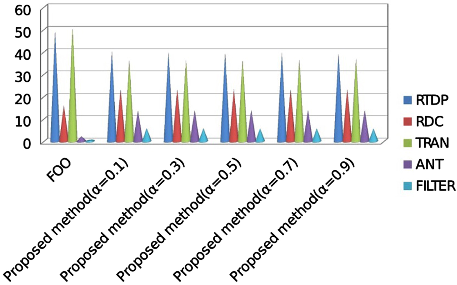
Comparison of allocated failure rate using two methods.

The results of FOO technique (Table 3) show that the allocated failure rates to RTDP and TRAN are high while the ANT and FILTER are less. By this technique, the allocated failure rate to FILTER is very less (0.266/10⁵h). Practically, to create a subsystem with such less failure rate would demolish a large quantity of resources which can affect the budget issue. But by our proposed method the allocated failure rate to FILTER is low, 5.690643495/10⁵h (at α = 0.5). So the required resources to produce a subsystem with this failure rate is remarkably less than those needed for FOO technique. Furthermore by FOO technique, the allocated failure rate of RTDP and TRAN indicates a high failure rate which leads to frequent failures and costly repair of the subsystem. But the failure rates obtained by the proposed method for RTDP and TRAN are reasonably less than the failure rate obtained by FOO technique.

So from all these assessments and figures, we can conclude that the proposed method is more realistic in apportioning the failure rate to the subsystems.

Several advantages of the proposed method:

Advantage in measurement scale:

Since the ordinal scale measurement is not meaningful, the operations of multiplication and division in FOO technique are meaningless. In our proposed method, we assume an equal numerical scale of rating and also normalize the matrix. So, the results by this method are meaningful and reasonable.

Advantage of ordered weight consideration:

The proposed method can assess the ordered weight of factors which the FOO technique fails to do. As the ordered weight of factors is one of the vital characteristic in reliability allocation, so the proposed method is more helpful to take a decision.

The proposed method can handle the prioritization of factors by considering different priority levels. But in FOO method, there is no priority consideration, means all factor are in same priority level. Thus, we can conclude that the FOO method is a particular type of the proposed method.

Finally, this method can deal with situation parameters values which is able to display the decision maker’s correct degree of optimism (strictly optimistic, moderate assessment, pessimistic) to flexibly aggregate the values of factors. However, the FOO technique does not consider situation parameters and so the decision maker mislead to take an incorrect conclusion.

A tabular representation of the comparison between the advantages of FOO technique and the proposed method is summarised in Table 10, where ’✓’ denotes that the related feature is considered and ’×’ indicates that the related feature is not considered.

Table 10

Comparison of proposed method and FOO technique

		Special feature
	Measurement scale	Order weight	Prioritization	Situation parameter
Proposed Method	✓	✓	✓	✓
FOO technique	×	×	×	×

7 Conclusion

This article clearly described the applicability of the proposed prioritized reliability allocation method. The flexibility of this approach is established here using an airborne radar system and a comparison is also made with the FOO technique. The main benefits from this proposed method are: 1) this method can handle effectively the ordered weighted problem and measurement scale problem; 2) It can efficiently cover the priority of factors; and 3) In this proposed method, reliability allocation factors are not restricted only in I, S, P and E, but also it can consider different factors like cost, risk, maintenance, complexity etc.

Hence this method can be utilized as a part of a wide range of different fields and industries which encourages the decision maker to determine a suitable allocation of resources in a system. Here the rating of allocation factors with respect to different subsystems have been considered as a crisp value. But sometimes experts can give their opinion as a fuzzy information like very high, high, medium and low. Therefore, consideration of fuzzy linguistic information with this proposed method is an important future scope.

Footnotes

Author biographies

Dr. Aniruddha Samanta is an assistant professor of department of mathematics, NSHM Knowledge Campus Durgapur. He is an active researcher in the field of reliability engineering & operations research. His areas of research are reliability optimization, multi-criteria decision making, soft computing techniques etc.

Dr. Kajla Basu is a professor of department of mathematics, National Institute of Technology Durgapur. She has published many research articles in reputed international journals. Her areas of research are operations research, fuzzy mathematics, statistical analysis etc.

References

AGREE. (1957). Reliability of military electronic equipment, washington, D.C.: U.S. govt. print. off. 4-377.

Bona,

G. D.

, Falcone,

, Silvestri,

, & Forcina,

(2018). IFM target.: an innovative method to define reliability target for prototype systems. International Journal of Advanced Manufacturing Technology, 95(9), 3349–3367. doi: https://doi.org/10.1007/s00170-017-1438-z

Bracha,

V. J.

(1964). The methods of reliability engineering. Machine Design, 7, 70–76.

Chang,

Y. C.

, Chang,

K. H.

, & Liaw,

C. S.

(2009). Innovative reliability allocation using the maximal entropy ordered weighted averaging method. Computers and Industrial Engineering, 57(4), 1274–1281. doi: https://doi.org/10.1016/j.cie.2009.06.007

Chen,

S. M.

, & Wang,

C. H.

(2009). A generalized model for prioritized multi-criteria decision making systems. Expert Systems with Applications, 36(3), 4773–4783. doi: https://doi.org/10.1016/j.eswa.2008.06.021

Chen

, Zheng,

, Liao,

, & Feng,

(2015). A multi-attribute reliability allocation method considering uncertain preferences. Quality and Reliability Engineering International, 32(7), 2233–2244. doi: https://doi.org/10.1002/qre.1930

Covino,

, Rodgers,

, Smith,

, & Clarkson,

(2000). Assessing reliability in mechanical systems. Journal of Integrated Design and Process Science, 4(2), 67–84. doi: https://dl.acm.org/doi/abs/10.5555/1240306.1240311

Felice,

F. D.

, Falcone,

, Silvestri,

, & Bona,

G. D.

(2010). Proposal of a new reliability allocation methodology: The integrated factors method. International Journal of Operations and Quantitative Management, 16(1), 67–85.

Hu,

, Chen,

, Wang,

, & Xie,

(2019). A new and practical reliability allocation method for a complex system of NC turrets. Mathematical Problems in Engineering, 2019, 1–10. doi: https://doi.org/10.1155/2019/1036729

10.

Kuo,

H. E.

(1999). Reliability assurance: Application for engineering and management(2nd ed.). Chinese Society for Quality. 3/16-3/17.

11.

Liang,

, Dong,

, Yi,

, Qin,

, Yang,

, & Hou,

(2018). Reliability allocation of multi-function integrated transmission system based on the improved AGREE method. Engineering Asset Management: Lecture Notes Mech Eng, 10, 155–166. doi: https://doi.org/10.1007/978-3-319-62274-3^.13

12.

Liaw,

C. S.

, Chang,

Y. C.

, Chang,

K. H.

, & Chang,

T. Y.

(2011). ME-OWA based DEMATEL reliability apportionment method. Expert Systems with Applications, 38(8), 9713–9723. doi: https://doi.org/10.1016/j.eswa.2011.02.029

13.

MIL-HDBK-338B. (1988). Electronic reliability design handbook, department of defense of USA.

14.

Ronchieri,

, & Canaparo,

(2018). Metrics for software reliability:a systematic mapping study. Journal of Integrated Design and Process Science, 22(2), 5–25. doi: 10.3233/jid-2018-0008

15.

William,

, & Alven,

(1964). Reliability engineering:ARNIC research corporation. Prentice-Hall, Inc., Englewood Cliffs, NJ, U.S.A.

16.

Yager,

R. R.

(2004). Modelling prioritized multi-criteria decision making. IEEE Transactions on Systems, Man, and Cybernetics, 34(6), 2396–2404. doi: https://doi.org/10.1109/TSMCB.2004.837348

17.

Yager,

R. R.

(2008). Prioritized aggregation operators. International Journal of Approximate Reasoning, 48(1), 263–274. doi: https://doi.org/10.1016/j.ijar.2007.08.009

18.

Yan,

H. B.

, Huynh,

V. N.

, Nakamori,

, & Murai,

(2011). On prioritized weighted aggregation in multi-criteria decision making. Experts Systems with Applications, 38(1), 812–823. doi: https://doi.org/10.1016/j.eswa.2010.07.039

19.

Yu,

, Zhang,

, Ran,

, Li,

, & Wang,

(2018). A comprehensive and practical reliability allocation method considering failure effects and reliability costs. Eksploatacja i Niezawodnosc –Maintenance and Reliability, 20(2), 244–251. doi: http://doi.org/10.17531/ein.2018.2.09

A prioritized decision making method for reliability allocation: In optimistic and pessimistic view

Abstract

Keywords

1 Introduction

2 Reliability Allocation Methods

2.1 FOO technique ((MIL-HDBK-338B, 1988); (Chang et al., 2009))

3.1 Ordered weight averaging operator (OWA operator)

4 Prioritization of criteria (Yan et al., 2011)

Table 1 Priority hierarchy of a set of criteria C Priority level Criteria H 1 C 11 ... C 1k ... C 1N .... ... ... ... .... ... H q C q1 ... C qk ... C qN q ..... .... .... ... ... ... H Q C Q1 ... C Qk ... C QN Q

6 Case study

Footnotes

Author biographies

References

Table 1
Priority hierarchy of a set of criteria C

Priority level Criteria

H ₁ C ₁₁ ... C _1k ... C _1N

.... ... ... ... .... ...

H _q C _q1 ... C _qk ... C _{qN
_q}

..... .... .... ... ... ...

H _Q C _Q1 ... C _Qk ... C _{QN
_Q}