
Abstract
Despite recent improvements in collected drilling data quality and volume, the actual number of wells being used in studies remain low and are often limited to a single source and oil field, producing results that are prone to overfitting and are non-transferable.
In our study, we access oil drilling data from 5 of more than 20 oil drilling companies collected from 2005 to 2016 from our industrial partner to create well drilling duration models for well planning. This project could lead to the creation of more generalized models from larger datasets than others in literature. However, the data is difficult to process without expert knowledge, further complicated by properties such as unharmonized, source-locked, semantic heterogeneity, sparse and unlabelled. Conventional automated methods for feature selection, propositionalization, multi-source, or block-wise missing techniques could not be used.
In this paper, we describe our method to assist the Knowledge Discovery in Databases (KDD) Selection stage of the abovementioned data - Feature Selection before Propositionalization (FSbP) via Database Attribute Health Feature Reduction (DAHFR) and Report Feature Correlation Matrix (RFCM), collectively known as FvDR. DAHFR and RFCM are filter-type feature selection techniques that could measure relational missingness and keyword correlations respectively despite the complexity of multi-source oil drilling data. FvDR successfully reduced the scope from 700 tables containing 20,000 columns to 22 tables containing fewer than 707 columns while successfully selecting 13 of 16 relevant tables suggested by literature. Despite the loss of information from limitations of subsequent KDD procedures, preliminary models show promising results with over half the test predictions falling within the 20% error margin required for well planning. FvDR proves to be indispensable in KDD as a FSbP framework as it reduces features for examination and streamlines the research process necessary to understand business rules for data harmonization and propositionalization.
Keywords
Introduction
Oil and gas exploration is a high risk, high rewards endeavour which requires a combination of specialized workforce and equipment to explore, plan and drill oil wells to extract crude oil and natural gas from oil fields. In recent years, oil drilling companies must contend with the high cost of oil drilling, where the cost of renting an offshore drilling alone could cost upwards of USD500,000 per day, the declining numbers of reservoirs which are easy to access while providing high yield, and the declined price of crude oil (during the time of the study). To economize well drilling operations, research is focused on methods to optimize the speed, safety of drilling processes and to provide benchmarks to measure the project’s progress.
Although mathematical models are still being created, most studies are now data-driven, taking advantage of recent drilling data from oil drilling companies which are steadily increasing in volume, scope, and quality with the advancement of data collection and storage technologies (originally used for reporting and progress tracking). The data-driven nature of these models leans their targeted usage to be close to where the data is collected, specifically as real-time predictive models during live drilling operations.
However, all the recent data-driven studies are limited in nature, with most available research papers using a subset of the available data collected from the drilling of one or a few local wells. Very few papers have access to data from an entire oilfield. From a machine learning perspective, the final model will be overfitted to that local oilfield, because patterns in oil drilling are defined by geological formations and the depth of formation transition.
In our study, we are grateful to our industrial partner, Independent Data Services for the access to oil well drilling data from 5 drilling companies and their oilfields. Independent Data Services provides data storage, reporting, and analytical services to more than 20 oil drilling companies. The data is collected over the duration of 10 years, from about 2005 to 2016 and provides an opportunity to create predictive models with more data than other available studies both in the number of wells and the number of available training features. The objective of the study is to create a phase duration prediction model from the data which could be used to aid well planners.
A defining problem in our KDD of this multi-sourced oil drilling data is the encountered in the Selection stage of KDD (Fig. 1). It is the nature of the available oil drilling data (relational, unharmonized, heterogenous, sparse, unlabelled (requires propositionalization), multi-sourced) as well as the unavailability of expert knowledge. This environment impedes manual or automated Selection and Transformation stages of KDD, of which Transformation must be performed before the data could be used for machine learning.

The KDD Process.
We address this problem by performing Feature Selection before Propositionalization (FSbP) via Database Attribute Health Feature Reduction (DAHFR) and Report Features Correlation Matrix (RFCM), collectively known as FvDR. The reduction in project scope via FvDR is essential for a timely project completion, as the addition of each of the 20,000 possible features in 700 tables (per database) in 5 databases (sources) into the scope is an increase in time complexity – time is required to individually examine, study, and identify the feature’s viability, and then transform it.
This paper is divided into 6 chapters. In the Introduction, we have described the opportunity which motivates this project and briefly described the problems which come with this opportunity. In Background and Motivation, we further describe the motivation for the use of multi-source data as well as the difficulties of using multi-source oil drilling data. In Methodology, we describe the FvDR framework and model evaluation method used during our KDD of multi-sourced oil drilling data. FvDR uses the combination of two novel Filter Feature Selection (FS) methods, DAHFR Ting and Then (2022) and RFCM which can be used without the need to transform the relational data. DAHFR is a filter feature selection metric that measures the quality of data in the form of relational missingness, while RFCM produces a correlation chart of features to represent business rules based on business reports produced from the database. In Results, we reveal the feature scope reduction rate performed by FvDR in the form of % of features selected, visualization of FvDR data, the selected features compared against features recommended by literature and the resulting models’ performance. In Discussion and Future Work, and Conclusion, we discuss the efficacy of FvDR both as a FSbP process and as a research tool in the multi-sourced KDD pipeline, areas for further improvements both for FvDR and our KDD process and place our concluding remarks on this paper.
Using Multi-source Data From Multiple oil Fields to Improve Generalization
Recent data-centric literature in oil drilling have been taking advantage of improvements in data collection technology such as Mud Logging and Wireline Logging, which increases the volume, reliability, and frequency of data collection. However, these literatures tend to be limited to data from a low number of wells, often involving just one up to a hundred wells or oil fields while data from multiple oilfields or more wells (2000 wells for Brett and Millheim (1986)) are rare.
The use of low number of wells and oil fields is problematic. There are at least two factors that can cause overfitting or overfitting-like issues when using data from only one oil field.
Most importantly, formation characteristics (Anemangely et al., 2018) and the depth of transition of formations define the planned well dimensions and drilling plan. During normal drilling operations, the unreinforced section of the well is stabilized by the weight of the mud which must follow a Safe Mud Weight Window (Gholilou et al., 2017; Ma et al., 2019), which changes from formation to formation. These depths of transition define depths drilling must be stopped to install (Al Ramadan et al., 2019; Byrom, 2014) and cement in place (Ahmed et al., 2019; Soares et al., 2017) a casing or liner down to the new depth which serves to isolate and reinforce the well from the surrounding formation.
It is to be noted that there is another methodology, where casing drilling is performed (Mohammed et al., 2012; Steppe et al., 2005). In this process, the casing also serves as the drill string (the moving component transferring torque from the surface to the drill bit) and the drill bit is attached to the end of the casing.
The availability of formation characteristics and depths data makes the difference of speed and cost of exploratory/appraisal wells versus regular development/production wells. Exploratory/appraisal wells must be drilled slower and carefully with limited formation information to gather the information. Development/production wells have advanced knowledge of safe and unsafe depths from offset (nearby, any type) wells and could be operated at speed until the unsafe zone is reached.
A second factor which is affected by rigs and oil fields is crew efficiency (Adeleye et al., 2004; Amorim et al., 2019; Anemangely, et al., 2018; Brett & Millheim, 1986; Hossain, 2015; Kaiser, 2007; Lukawski et al., 2014; Whelehan & Thorogood, 1994) even though many papers have limited features available and must perform predictions without experience data or predict the Rate of Penetration (ROP) using only wireline data (Abtahi et al., 2011; Amar & Ibrahim, 2012; Hamrick, 2011; Huang et al., 2011; Paiaman & Moghadasi, 2009; Sultan & Al-Kaabi, 2002). Adeleye et al. (2004) talks about how experience and better information allows drilling performances to approach the Best Composite Time (best predicted time) of a drilling operation. Lukawski et al. (2014) and Amorim et al. (2019) tells of how experience from drilling offset (nearby) wells will improve decision making on the choices of drill bits to be used for drilling through the formation, better insight into the site’s lithology or simply eliminate past mistakes from being repeated.
By using data from wells of one oil field, data will be overfitted to the formation characteristics (and their drilling properties) and decisions made in the formations for that oil field and the experience of the crew operating in that oil field (which improves the more wells they drill in the same field). This leaves an issue in transferring this knowledge to a new oilfield, where the crews are different, and the depths of different formations and transitions are different.
Multi-source Oil Drilling Data is Difficult to Propositionalize
The use of multi-sourced oil drilling for KDD is a double-edged sword. While the usage data from multiple sources improves the generalization ability of the resulting model, the amount of work to prepare the data increments with each source, as work must be done to individually examine and study the sources, and them merge them into a harmonized dataset.
In this section subsections, we’ll be using LazyBum (Schouterden et al., 2019) as a baseline when discussing difficulties handling multi-sourced oil drilling data. LazyBum is a lazy variant of the One Button Machine, which automatically converts tables in relational databases into a propositional dataset, while handling one-to-many and many-to-many relationships without the need for expert knowledge.
Sparse Data Causes Block-Wise Missing Data in Multi-source Data
During preliminary work on the underlying data, the absence of an Entity Relationship (ER) model makes it difficult to compile relevant data. Manual and automated inference of the ER diagram makes joining possible, but several sparsity issues interfere with the process which causes rows of data to be dropped when intermediate tables turn out to be unused or barely used. These issues stemmed from various causes: some tables were filled mostly or exclusively with test data, some data were available only in random cases with whole rows missing at seemingly random rates, and some data were missing at the feature level, interfering with initial aggregation attempts.
LazyBum already handles this problem by automatically aggregating missing data as part of its propositionalization process, but the block-wise missing data created could not be dismissed. When the multiple sources are merged, it creates a dataset where entire groups of features are empty (depending on the source), a situation called block-wise missing data.
In literature, block-wise missing data is often encountered in heterogenous multi-source clinical data, where study, test, or departmental data are joined on the individual patients (Li et al., 2019; Xiang et al., 2014; Xue & Qu, 2021; Zhu et al., 2020). Block-wise missing data occurs when the patient data is not available in some of the sources, of which the sources represent entire feature sets being missing for groups of patients.
There are two main strategies of dealing with heterogenous multi-source data and its resulting block-wise missing data. The first strategy is to divide the main dataset into multiple subsets that are less afflicted by sparse data and then either impute them (Xue & Qu, 2021) or train multiple learning algorithms and rejoin the algorithms into one (Li et al., 2019; Xiang et al., 2014). Otherwise, the data is not divided, and imputation is performed anyway (Du et al., 2023; Zhou et al., 2021; Zhu et al., 2020), or machine working frameworks that works with block-wise missing data are used (Ghorpade-Aher & Sonkamble 2022).
However, examination of the characteristics of multi-source oil drilling data shows that it is closer to being homogeneous multi-source data than heterogeneous. Homogeneous multi-source data are data from different sources that are identical in format and attributes (Wu et al., 2017). They usually consist of sensor data or data from multiple studies of the same subjects, and objectives include the fusion of the data into a singular dataset for further analysis, which often requires harmonization. Difficulties during the fusion process tends to be attributed to differences in semantics, sensor settings, and entity identification. Missing data are barely mentioned in homogeneous multi-source data studies, and block-wise missing data are not mentioned at all (Li et al., 2017; Misiuk et al., 2020; Zhang et al., 2019; Zhang et al., 2022).
A key difference between oil drilling data versus heterogeneous or homogeneous multi-source data is the data distribution. Homogeneous studies aim to create datasets by unioning cases, while joining cases that represent the same entity. Heterogeneous studies perform the same, except with features instead of entities. Even though harmonization may be required for homogeneous or heterogeneous (Dinov et al., 2016; Kaiser et al., 2024) multi-source data, in the homogeneous or heterogeneous cases, some of the data are connected cross-source to provide a basis for comparison and missing data recovery.
Ultimately, block-wise missing oil drilling data could not be handled in the same manner as those encountered from other heterogeneous or homogeneous (non-existent) sources found in literature. Regular heterogeneous multi-source data in literature involve data taken from the whole population, so training or imputation could be made with the existing biases (confidently representing the global bias and distributions). However, because of the non-overlap of well/oil field data across sources and the unavailability of some data (specifically formation data) and the difficulty in comparing data across oilfields as mentioned in chapter 0, block-wise missing oil drilling values could be unrecoverable.
For for the lack of a better name, we differentiate the oil drilling data used in this study as ‘source-locked’ homogeneous multi-source data to represent its distinctiveness from other multi-source data and the need for different strategies and decisions in response to the resulting block-wise missing data.
Harmonization and feature engineering
Despite the availability of automatic propositionalization techniques like Lazybum, the variety of data that are available could cause issue. Plenty of the data require expert knowledge or additional techniques to convert it into usable data. For example, activity data is a treasure trove of information but requires natural language processing to extract further information and is an entire field on its own (AbouLaban et al., 2022; Castiñeira et al., 2018).
In this project, several propositionalization and harmonization techniques require expert consideration and research to properly transform the data to make it useful for machine learning, while keeping it comparable when merging multi-source data. To get the label (phase duration), irregular-length time-series activity data must be merged into phases, which must then be harmonized into standardized phase set (Figs. 2, 4a, 4b). This data must be joined with other time series data (aggregated daily, or irregular-length as well) and relational data. The bharun data must be harmonized as well to standardized categorization of bha types, then based on the bha type, decisions must be made on whether they should be joined to a given phase (Fig. 4d). Bit types are often uncategorized to the point that rules from expert knowledge and machine learning must be employed to fill in areas of confidence (Fig. 4c). Hole dimensions must be examined from multiple time-series data related to the operation due to sparsity (Fig. 3), to determine one given diameter of a particular hole or casing section. Many of the underlying data could not be propositionalized without expert knowledge.
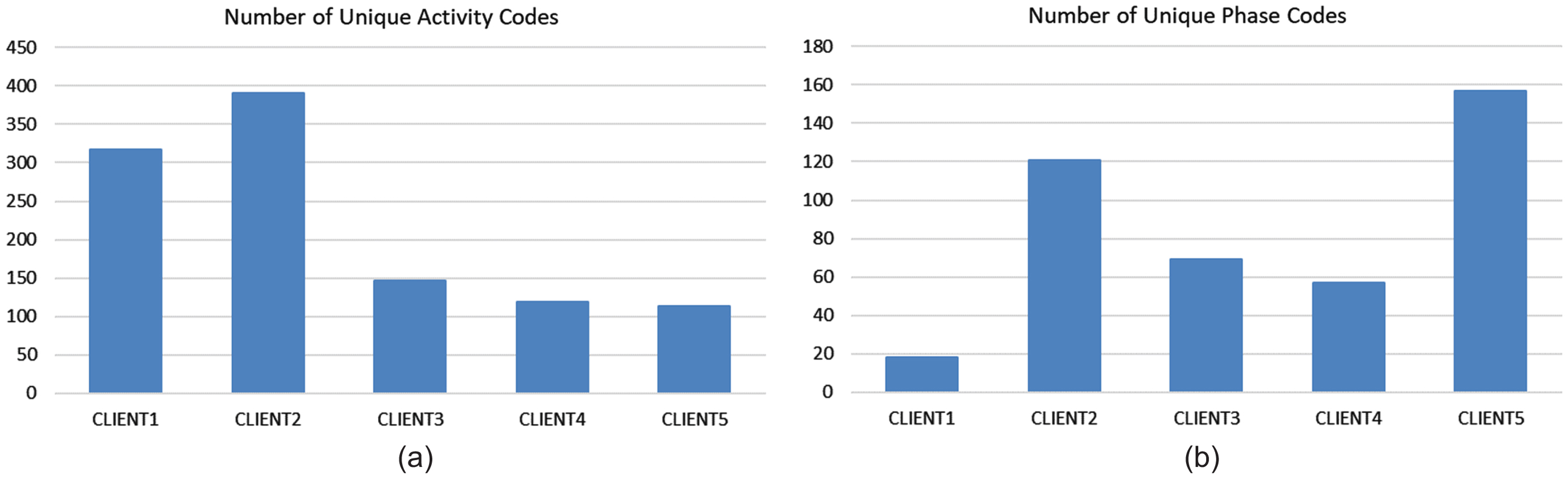
Number of Unique Activity (a) and Phase (b) Codes That Must be Harmonized Across Sources.
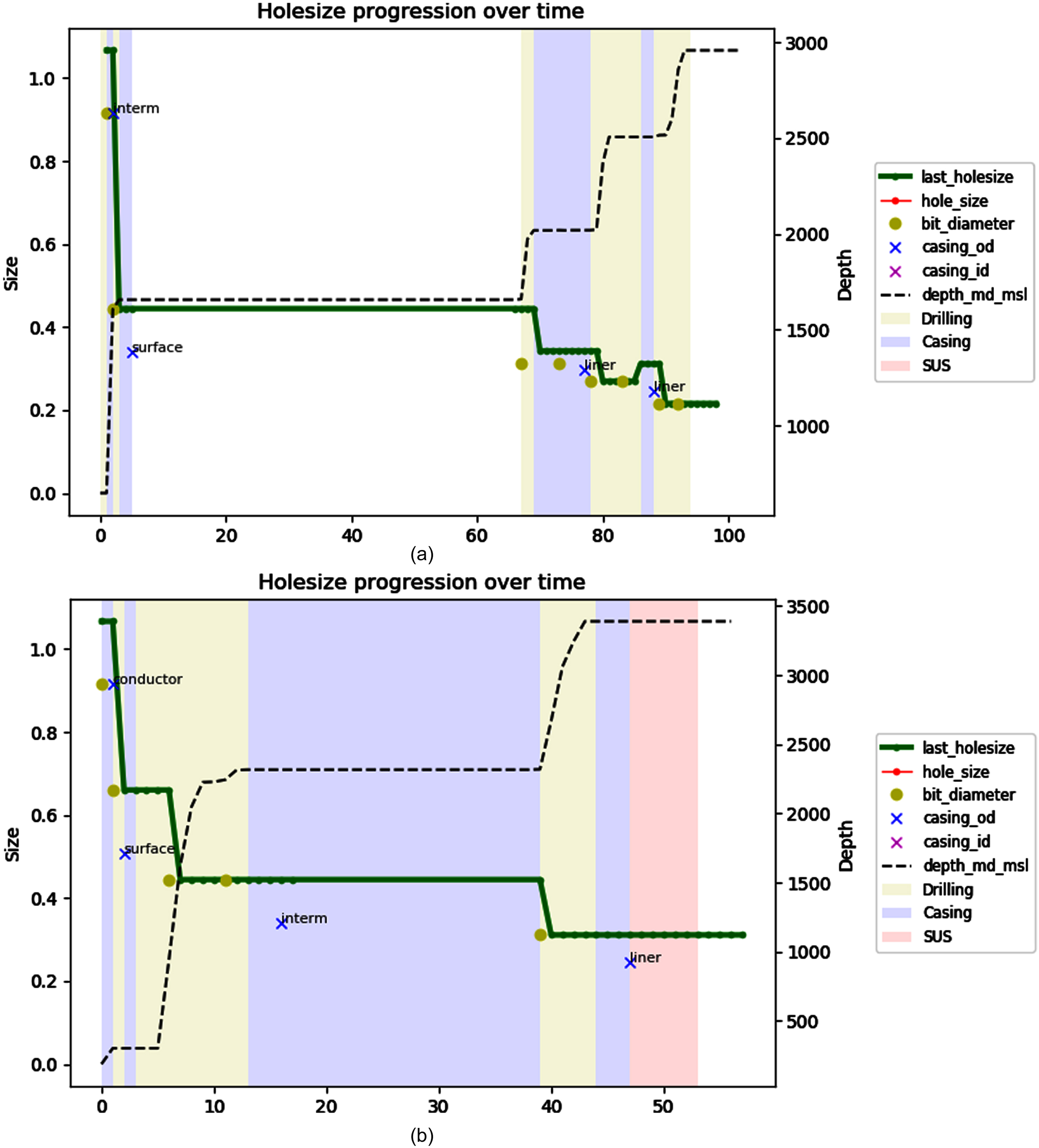
Hole Sizes, Phase and Depth over Time for Operations in DB4. Each Legend Represents a Different Hole Size Data Source: report_daily.last_holesize (daily time-series), activity.hole_size (irregular time-series), bitrun.bit_diameter (once per bitrun), casing_section.casing_od & casing_section.casing_id (outer or inner diameter of casing, once per casing/liner run). Data is Compared to Identify the Singular Hole Size for any Given Phase (Drilling, Casing/Liner) (Conductor, Surface, Intermediate, Production).

Various Data Processed. (a) Standardizing Phases (b) Merging Standardized Phases (c) Missing or Miscategorized Bit Type Problem (d) Standardizing Bha Types and Associating Them to Phases.
In 2.2, we establish that automated propositionalization could not perform all the tasks required to propositionalize and harmonize multi-source oil drilling data. Manual examination and use of expert knowledge is still preferred to perform this task, but the research and work required is massive for each additional feature added to the dataset.
FSbP could aid in prioritizing features that are relevant by performing feature selection before data compilation. There are a few papers that focuses on this topic. Motl and Kordík (2018) performed FSbP by using meta-learners to perform a filter-method selection of meta-features (unpropositionalized features). In their study, the meta-features are measured based on their relevancy to the task, feature redundancy, and runtime of feature calculation. Krogel and Wrobel (2002) on the other hand, used the wrapper method to perform feature-selection by relying on the available schema and label to automatically propositionalize the target feature to the label to determine the feature’s relevance.
Both papers rely on the capability to relate meta-features to the label to measure its relevance to the task. However, as discussed in 2.2, the labels are not available at the early stages of examination and the irregular time-series, need-to-harmonize and multi-source nature of the data makes it difficult to perform the comparison both on a per-source basis and on a multi-source basis. FvDR aims to perform FSbP without directly observing the data.
Methodology
FvDR is performed in four steps as seen in Fig. 5 as part of the KDD of Multi-source Oil Drilling Data:
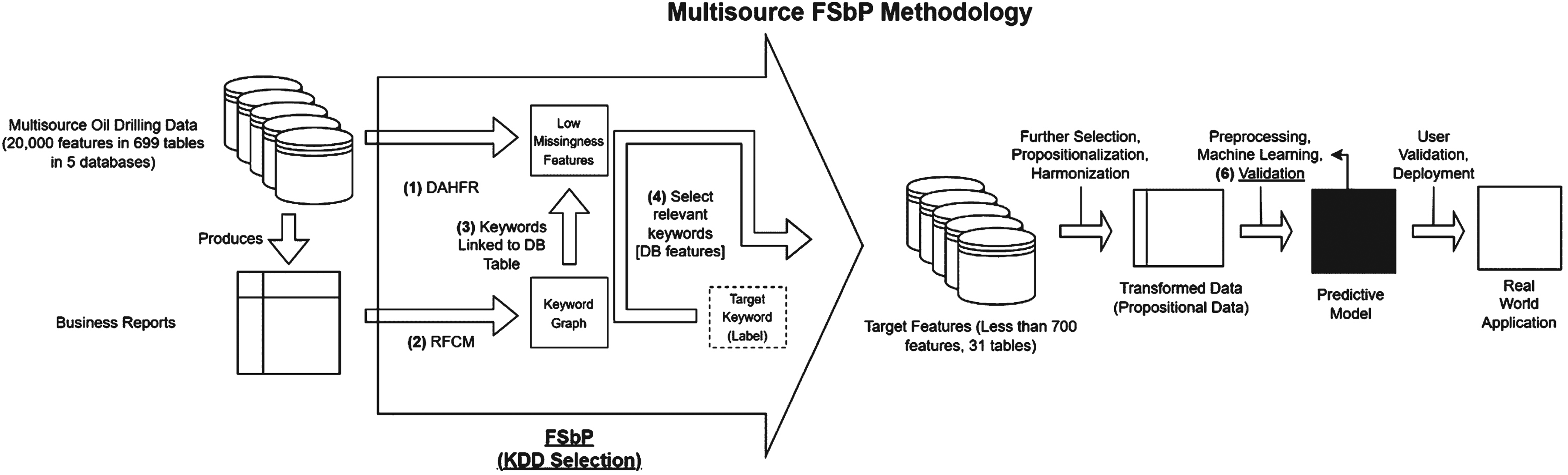
The FvDR Process for Multi-Sourced Oil Drilling Data.
Database Attribute Health Feature Reduction (DAHFR) (Ting & Then, 2022) removes unused or extremely sparse multi-source database features from the project scope.
A report Feature Correlation Matrix (RFCM) is created from business reports generated by the system. Feature Correlation data from RFCM serves as a representation of expert knowledge to identify concepts that are relevant to a target machine learning objective.
The keywords from RFCM are related to database features found in DAHFR.
Relevant database features are identified by tracing RFCM keywords that are relevant to the target label.
These steps and the evaluation method are described further in the following subchapters.
DAHFR is a Filter type Feature Selection metric we created which identifies which tables and columns ‘contain enough data’ which in our multi-sourced data project, is also used to perform the comparison across multiple databases. Instead of examining the table-rows for missing data, DAHFR uses ‘relational missingness’ (Fig. 6) as a metric to estimate how many % of the data will missing for the given feature or table after data has been propositionalized. The following are the steps to perform DAHFR.
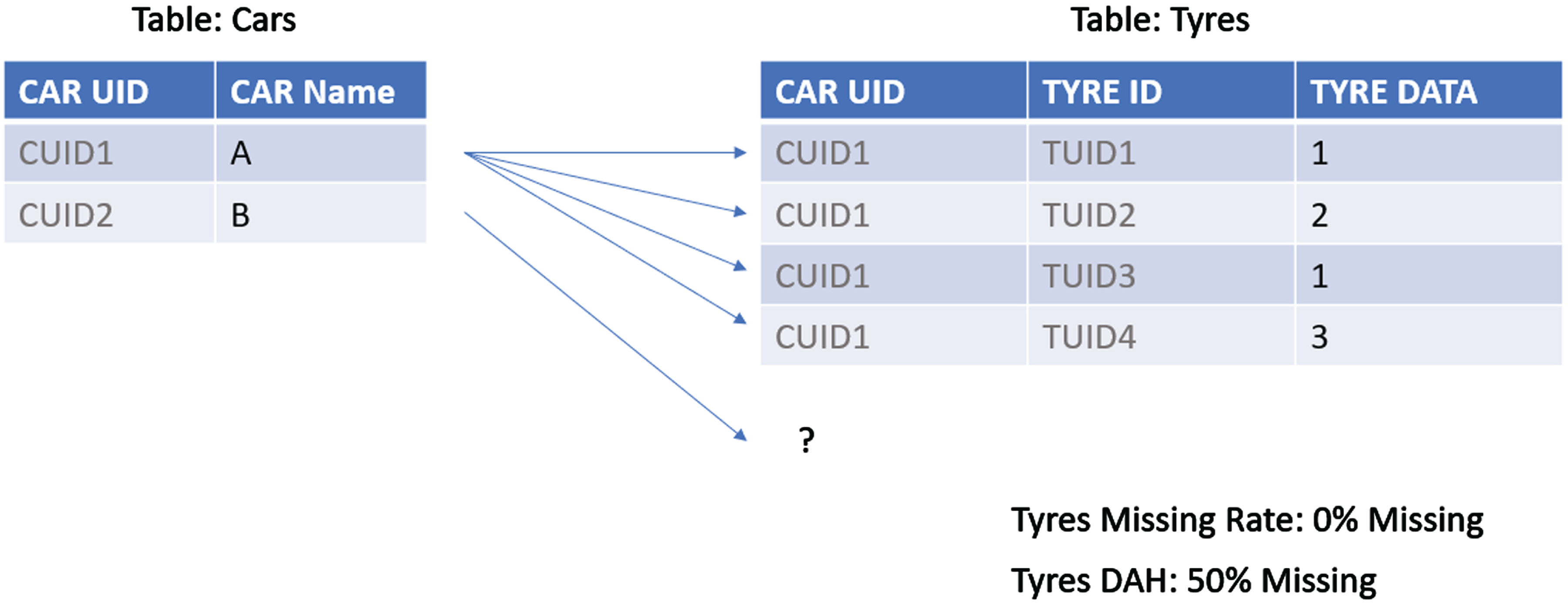
DAHFR Rationale for Relational Missingness.
A baseline feature is selected for measuring the DAH score. The feature is selected based on the following characteristics:
Is a Foreign Key: For easier cross-table comparisons, while ensuring that the values being compared are unique. Relatability: It must be relatable to as many tables as possible. Granularity: It must contain a high number of unique values to be able to obtain a final resolution of the DAH score. Meaningfulness: The definition of the baseline feature should be significant and easily interpretable, eg: x% of baseline feature y are represented in feature z
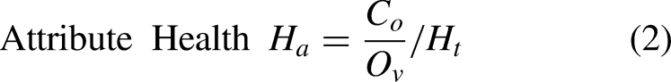
For each table, its relationship to the target label is traced to baseline feature. The DAH (consisting of H
t
(1) and H
a
(2)) are measured. O
t
= count of distinct, valid baseline uids represented by the table. O
v
= count of valid baseline uids in the baseline table. C
o
= count of valid baseline uids represented by the column. A baseline uid is represented when at least one row holding the baseline UID contains data in the column. Relational missing % = 1 – Health

Features with poor scores are reduced using the threshold specified in Table 1. This threshold is based on the user’s decision. In this project, several factors were considered. Firstly, the actual missing rate after propositionalization will higher than the DAH due to the ‘one row or more = 1 weight’ rule. Second, a low table health threshold is employed because MNAR (Missing Not at Random) data can significantly skew results. Examples of observed tables that are significant but have low table health, tables that record events (rare, causes delays or even casualties) and drilling data (a source contains many operations but only 45% of the operations are drilling operations).
DAHFR Threshold Used in a Single-Source and Multi-Source for This Study.
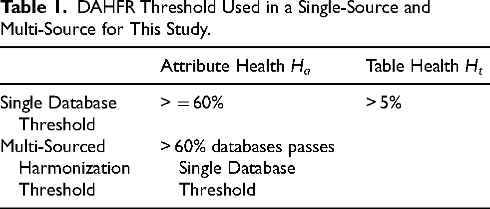
DAHFR Threshold Used in a Single-Source and Multi-Source for This Study.
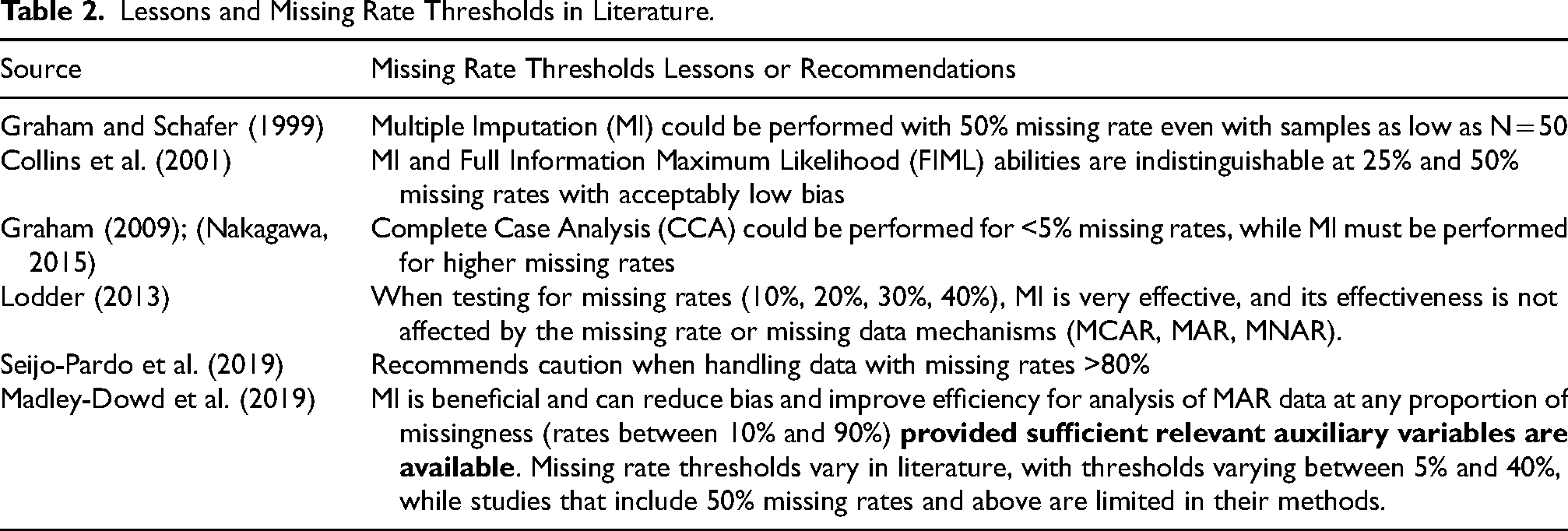
Although skipped in this study for the sake of reduced complexity (due to complexity in dealing with missing data at a source-locked multi-source level) there are further considerations in the realm of missing data. A low Attribute Health or Missing Rate is a complex issue in missingness. (Poor) Missing rates does not inform the user on how well the missing data could be recovered from the available observable data (Lang & Little, 2018). A consensus is that
Lessons and Missing Rate Thresholds in Literature.
The objective of Knowledge Discovery in Databases (KDD) is to transform secondary data (information collected by others for different purposes and then utilized in a study) into actionable knowledge. This process is particularly relevant for business-oriented databases, where the primary goal of collecting data is often to provide key stakeholders with insights into the business’s status through reports.
This implies that within the context of KDD, each database has an associated set of reports generated from its data. We can target these reports as a rich source for extracting correlation data, operating under the premise that the features used to generate these reports are either correlated, or thought to correlate to other features within the report. These reports, created by experts could therefore mirror some of their business knowledge in the form of the correlation data.
Given this framework, the process of extracting correlation data from reports presents a scalable and repeatable opportunity across different databases. This is because the generation of reports from data is a common practice across various databases, making this approach widely applicable and potentially valuable for gaining insights across multiple domains.
These are the steps used to perform RFCM. For this project, only the reports of DB4 (Source #4) are examined due to the time constraint. The schemas and reports are expected to be generally the same, although it is known that custom reports have been requested (generated manually) which are not available through the reporting website.
Examine System Reports and Gather Characteristics into Report Features Index (RFI)
Distinct business reports are generated by accessing test or staging websites for the system, ensuring the live data and websites are unaffected.
For each report, we identify several key components, as illustrated in Fig. 7. The
Sample Oil Drilling Reports and Keywords Gathered from DB4 Reports.
The keywords identified in the Report Features Index are searched for online and then grouped manually. Synonymous keywords are combined. When keywords fall under the scope of a more significant keyword, they are typically merged into this larger keyword, except in cases where the smaller keyword frequently appears in reports.
Convert the RFI into a Report Features Correlation Matrix (RFCM)
The RFI is converted into the RFCM, where the RFCM compares features based on how many reports they have co-occurred in. The RFCM provides an overview of the distribution and prevalence of features while providing the viewer with an analogy of business rules in the form of ‘feature closeness’.
Step 3: Linking DAHFR to RFCM
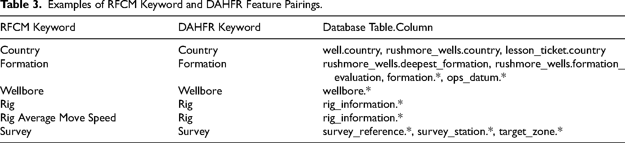
Using the knowledge gained during the RFCM process, the RFCM keywords (representing the business domain) are related to features (by column names or table names) from filtered from DAHFR as shown in Table 3. It is expected that the RFCM keywords may be related to several tables/columns, as RFCM keywords may be generated either directly from, or calculated from DAHFR features.
Examples of RFCM Keyword and DAHFR Feature Pairings.
Examples of RFCM Keyword and DAHFR Feature Pairings.
The relevant features from the database are gathered via the following steps.
Identify the label keyword (the KDD/ML objective) from the RFCM. Use the RFCM to search for keywords relevant to the label keyword. Using the links created in Step 3 to identify the label features, and relevant features from the DAHFR (database domain).
Steps 1 through 4 constitute the procedure for FvDR. In this paper, we use two methods to evaluate FvDR. The first method consists of the comparison of FvDR’s selection result, either as keywords or as features, versus features recommended by literature. The second method consists of running the entire KDD process, which includes manual selection, transformation (propositionalization and harmonization) and machine learning. The machine learning models are used to assess the FvDR’s effectiveness, which is the common method to compare the effectiveness of feature selection methods.
Results
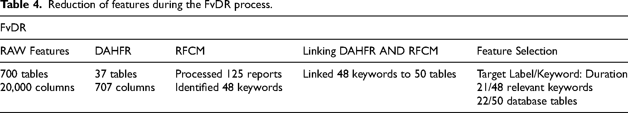
FvDR
During FvDR, the scope of features to observe is reduced from columns in 700 tables to 30 tables as seen in Table 4. This is a reduction of the scope to 4.3% tables of the original. DAHFR provides a significant reduction due to the very sparse nature of the multi-source oil drilling data. After the reduction, the DAH scores serve as an intuitive cheat sheet (Tables 5, 9) to allow the user to quickly identify relevant features or features of interest to examine, while also preventing potential MNAR data from skewing the result by allowing the user to focus on the Column/Attribute Health during comparison.
Reduction of features during the FvDR process.
Reduction of features during the FvDR process.
RFCM (Fig. 8) serves as a repeatable source of business knowledge to find keywords that are relevant to any target prediction objective. The process of gathering and merging keywords also serves as a scope-limiter, as it provides the user with a list of keywords relevant to the database to study in the expert-knowledge gathering process without needing to search too deep or wide until required (extensive expert knowledge is required for propositionalization and harmonization).

RFCM Produced From the RFI Comparing Co-Occurrence Counts of Keywords.
The rest of KDD was performed after FvDR. Of the 30 tables recommended by FvDR (Table 5), 8 were selected manually for Propositionalization and Harmonization. This is because of the difficulty in transforming the features, which is complex and time-consuming.
Visualization of DAH Scores for Activity (a) and Bharun (b) tables across 5 sources (db1-db5). A better score (green) suggests a lower relational missingness.
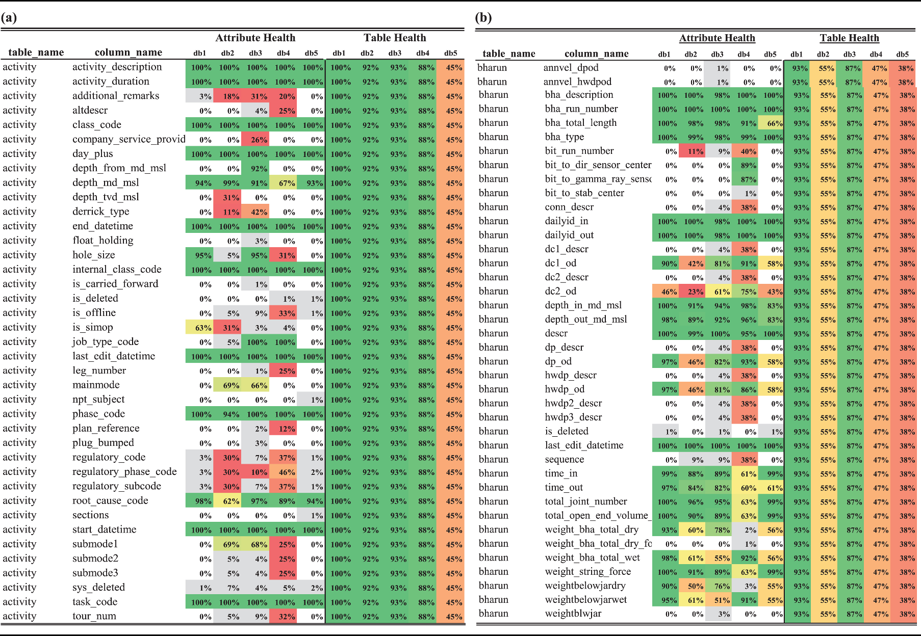
Visualization of DAH Scores for Activity (a) and Bharun (b) tables across 5 sources (db1-db5). A better score (green) suggests a lower relational missingness.
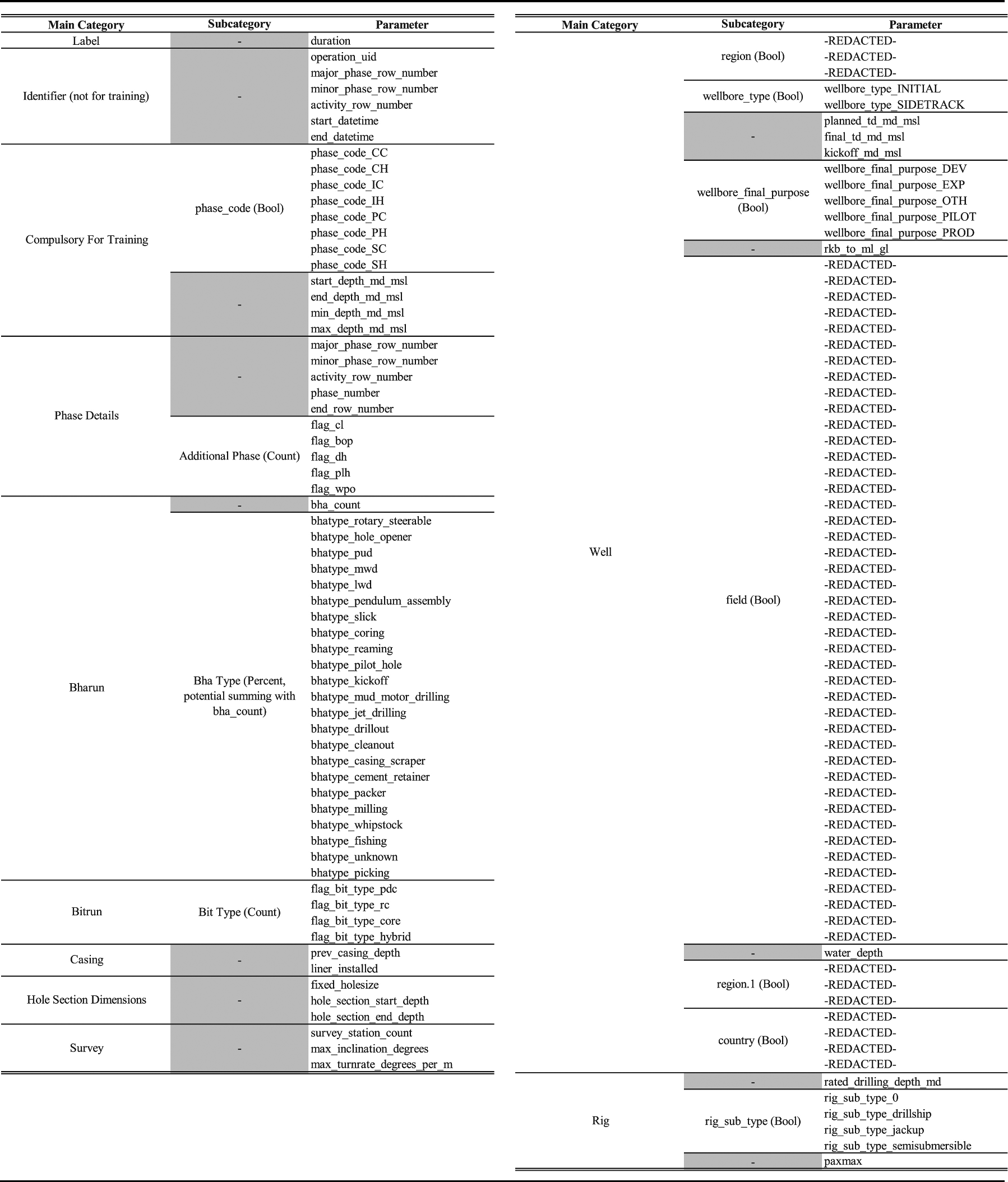
After KDD Transformation, the dataset (consisting of parameters in Table 6) was used for ML processes to predict the duration of oil drilling phases. The problem is treated as a regression problem with the use of RMSE to identify the best performing models.
Features/Parameter Available After Harmonization and Propositionalization.
Two rounds of ML were performed. The first ML involved the use of Deep Learning which was manually finetuned over many iterations to create the best model, but it did not perform better than the baseline model, which was the Random Forest Regressor. In the second round, the dataset was split in a ratio of 70/30 operations into a training set and test set accordingly. Although the prediction is to be made for the duration of phases (one operation has multiple phases), the separation prevents the contamination of data from the same operation, which is not available during well planning. The separation also makes it easier to create DvDs for each operation which are entirely training-validation or test results.
Multiple combinations of ML preprocessing are created and tested with three model types (Random Forest Regressor, Linear Regression, and Multi Layer Perceptron) with the model configuration left at default settings. Although not used for evaluation of FvDR due to the problem discussed in chapter 5.3.3, feature selection data were collected to identify the relevance of each parameter that were created in KDD Transformation (Table 7). This data provides an outlook whether certain data are more useful than others, and whether feature engineering using expert knowledge (conversion of some features into others) is worth the resources spent. For example, survey data, which are coordinates along the drilled oil well was converted to represent the complexity of the hole (survey_station_count, max_turn_rate_degrees_per_m, and max_inclination_degrees) and are considered important features for prediction by the FS algorithms (Table 7).
Top Performing Features Identified by FS Techniques After Harmonization and Propositionalization. Average Score Refers to the Average Score Across Model Combinations During Training.

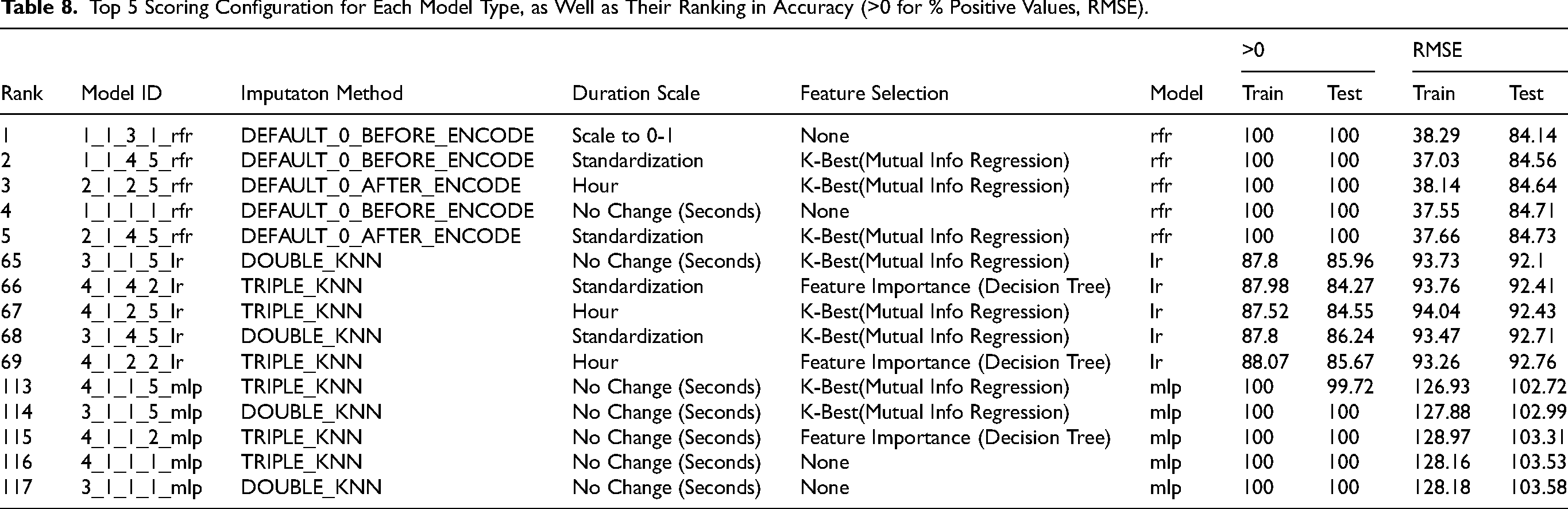
Ultimately, among learning algorithms available, Random Forest Regressor outperformed the rest of the models in both ML rounds, in both the RMSE score and the ‘larger than 0’ score (Table 8). The results of this best model are displayed and discussed in Chapter 4.2.2.
Top 5 Scoring Configuration for Each Model Type, as Well as Their Ranking in Accuracy (>0 for % Positive Values, RMSE).
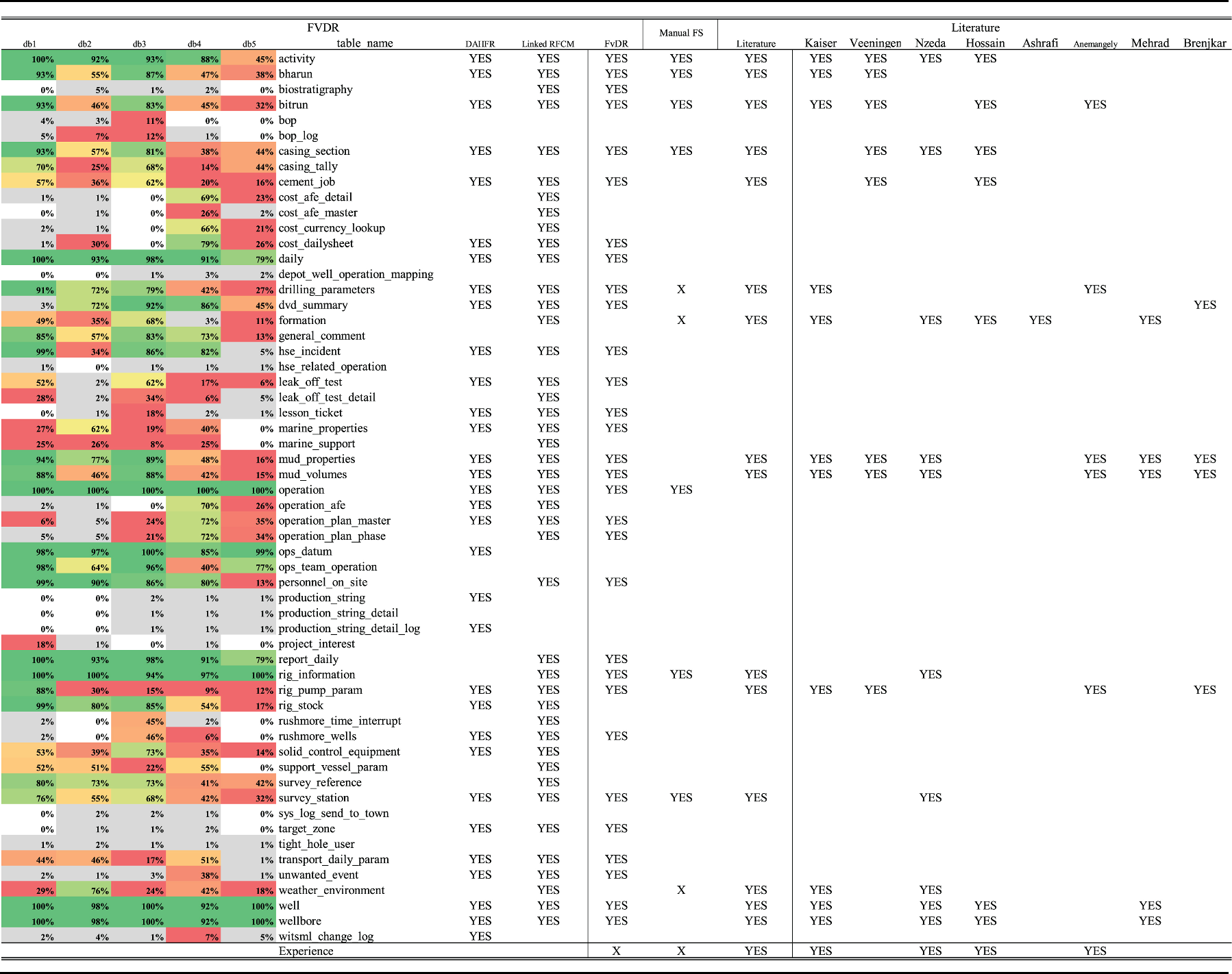
The first evaluation was done by comparing the FvDR’s selected tables against the tables suggested by literature (Table 9) that are relevant to the prediction of Rate of Penetration (a form of duration) and cost of drilling, which is directly affected by the drilling duration. Despite a reduction of scope from 700 tables to 30 tables in a multi-source environment, FvDR was able to identify 13 of the 16 tables recommended by literature. The following are the tables missed and explanations where only 1 of the tables missed is considered a failure in RFCM/FvDR.
Comparison of tables recommended by FvDR, Manual Selection, and Literature. YES refers to recommended tables/keywords, while X refers to tables or keywords that are unused with a reason. The literatures used are Anemangely et al. (2018); Ashrafi et al. (2019); Brenjkar et al. (2021); Hossain (2015); Kaiser (2007); Mehrad et al. (2020); Nzeda et al. (2014); Veeningen et al. (2009) which predicts either the cost of drilling or ROP.
Despite using only 8 tables of the 30 suggested by FvDR, the best performing model was able to estimate convincing DvDs that mimic the true DvDs of the operations (Fig. 9). To get a better estimate of the model’s viability, we use threshold of ±20% DvD duration error to be considered a successful prediction. The threshold is based on Hossain (2015) who says that operations should not exceed initial budgets by 20% and with the assumption that drilling cost is linearly related to the drilling duration. Based on the observation of training and testing cases, the accuracy increases as the length of the operations (and number of phases) and the number of phases in the operation and/or the duration of the phases increases (Figs. 10, 11). This is expected because the models trained were trained to minimize RMSE instead of percentage error.
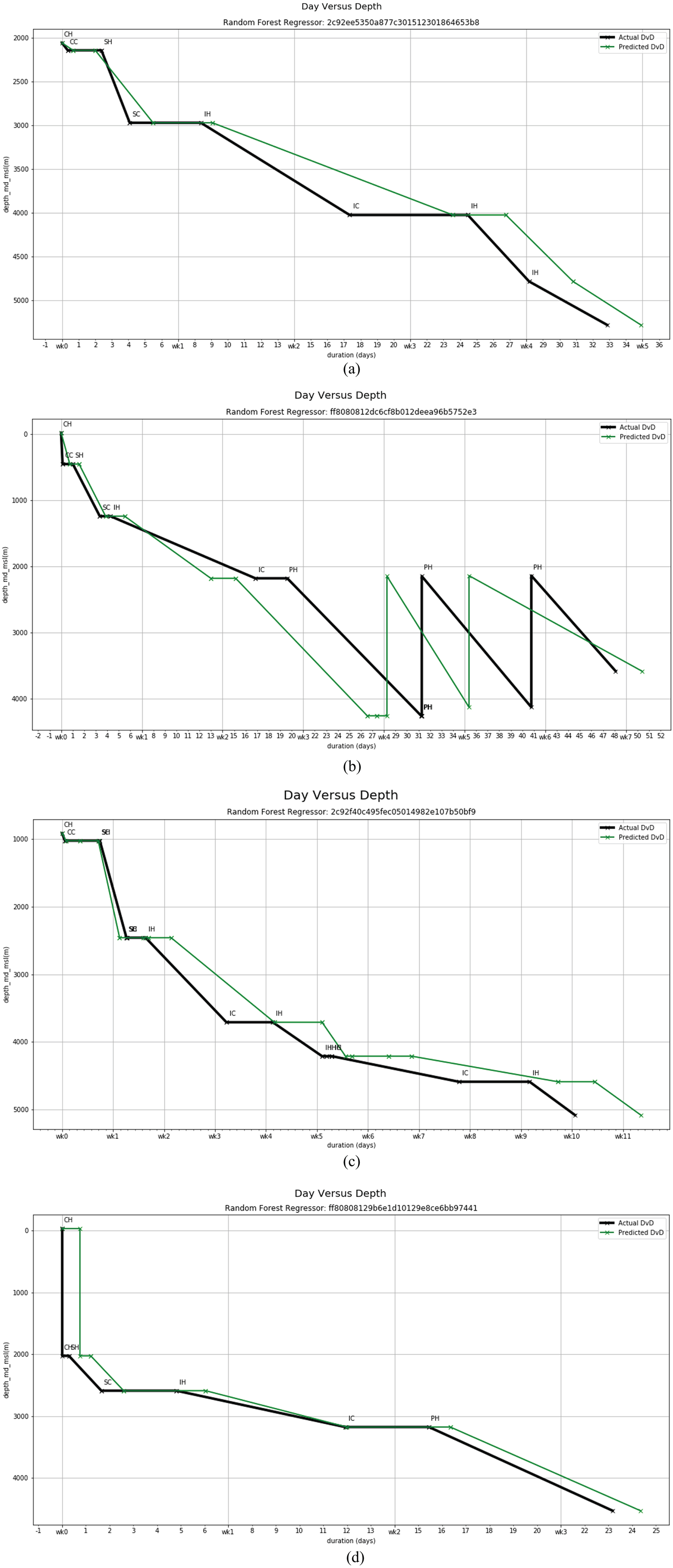
Sample Model Predictions of Well Drilling Duration.

Cumulative Count Comparing Successful Predictions vs Length of Actual Operation. Failure Rates were Expected to be Higher for Shorter Duration Operations due to Use of RMSE, but the Chart Shows the Distribution to be Relatively Stable.

Prediction Accuracy of Operation Duration Prediction Model. Dotted Lines Represent the ±20% Range Used to Determine the Accuracy.
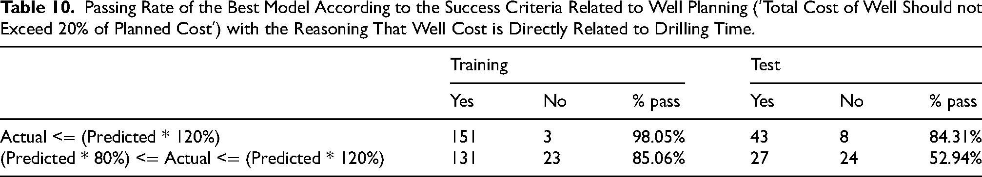
A total of 53% of test operation predictions falls within this threshold (Table 10) which shows some level of prediction success despite the limited number of features used to create the dataset.
Passing Rate of the Best Model According to the Success Criteria Related to Well Planning (‘Total Cost of Well Should not Exceed 20% of Planned Cost’) with the Reasoning That Well Cost is Directly Related to Drilling Time.
Limitations
During this project, several limitations are acknowledged:
Limited attempts at automated propositionalization were performed. It is possible that with more time and resource spent in building a framework of automated propositionalization, then harmonization, etc, that a better predictive model could be created without FvDR. Very few of the features selected by FvDR were used to create the dataset, due to the work required to add each additional feature as seen in background. In the same vein, the full effectiveness of FvDR is difficult to determine, given that FvDR’s effectiveness is entirely dependent on the predictive model, which is created after the data is processed several times over in the KDD process causing several stages of potential loss in information. The evaluation of the model’s ‘accuracy’ of RMSE is also non-ideal, as the prediction of any duration model is a probabilistic problem. Even in the oil and gas industry, duration prediction in well planning is done with the estimation of p10, p60 and p90 values (Coelho et al., 2005; Løberg et al., 2008) or probability distribution graphs (Adams et al., 2010; Codling & Leatherby, 2013; Moeinikia et al., 2014) for each phase, which are then used for monte carlo simulation to create probabilistic duration estimates.
FvDR has been instrumental as an entry point for the observation of multi-sourced oil drilling data. By reducing the scope of features to observe (from 700 to 30 tables), FvDR allows the database to be more manageable for the non-expert user to understand and study. In the case of multi-source oil drilling data where the features are often very sparse, DAHFR is important to identify features with ‘enough data’ for the user to use in follow-up decision making processes while providing a quick comparison across sources. RFCM also serves as a guide, not just by selecting the relevant keyword but for providing a scope of keywords to study, ensuring the non-expert does not spend effort in researching outside the scope.
As a FSbP process, FvDR must not only reduce the scope, but avoid removing relevant features in the process, while also not having the target label immediately available (it was feature-engineered during KDD Transformation). Preliminary results are promising. As observed in the Results, despite selecting only 4.3% of the possible tables, FvDR successfully selected 13 of the 16 tables suggested by literature, with only 1 of the missed tables being unexplainable.
As for the final predictive model’s accuracy, despite the limitations and loss of information in the rest of the KDD process, the final model was able to achieve a 52.94% success rate.
Future Work
DAHFR
DAHFR was created due to necessity when severe sparsity makes it difficult to identify which tables and features are worth examining in the database. With current work, DAH is already employed with limited success to identify less sparse data while hinting at the existence of MNAR data, as opposed to directly having MNAR data be the cause of entire features being dropped.
However, as discussed in chapter 3.1.3, missing data is a complex topic, but here are some statements and questions as food for thought.
MI is the best option for most cases, regardless of the threshold, MAR and MNAR debacle. While missing rate as a threshold is less relevant for MI (MI could still return acceptable results), the result of MI could be improved with the addition of expert knowledge and auxiliary data. DAHFR was initially created as a necessity, a method to view the extent of the sparsity in the database in the case where too little knowledge is available in the database.
Could DAHFR be modified to behave more like FMI (the better alternative to missing rate) without directly observing the data (which is a requisite for DAHFR)? Could DAHFR be used to better identify MNAR? From a single-source point of view, MNAR data could or could not be a problem when the availability of auxiliary data is not known (due to the unpropositionalized state), so should a threshold still be implemented?
When dealing with source-locked homogeneous multi-source data, the author asserted that the nature of the drilling data prevents the use of data from other sources from informing the imputation method. But to what extent is this correct, at various levels of ‘block-wise missing’ (eg: completely missing vs 95% missing) at source levels? There is room to study this in the future with the addition of more sources - only db4 was completely propositionalized and harmonized in this study so comparisons can’t be made.
RFCM
RFCM as a component of FvDR has found surprising success in identifying targeted, relevant feature groups (tables) when compared to features suggested in literature. At current levels, RFCM could only show correlation, but not the intensity of correlation between features and it is hoped that the improvements in this process could lead to better RFCM methods in the future.
By improving the correlation estimation and giving directions to the correlation, we hypothesize that RFCM could also be used to not only identify correlated data, but to outright estimate features that that predict the labels by first converting RFCM into a graph structure then searching for the Markov Blanket (Gao et al., 2015) of the target label.
Another area for improvement could be the automation of RFCM processes. Three areas could be automated in RFCM. First is the gathering of keywords, which must be done during the form-filling (to generate the report) and the resulting report, which could be done either by web and document crawling, or by image processing. Second is the grouping of keywords of similar nature. Third is the linking of these keywords to database (by identifying relevant keywords associated to the main keyword). It is possible with the increasing potency of Large Language Models, that the second and third step could be automated.
How do you compare FSbP versus other FSbP or FS techniques
In this project, the comparison in performance can’t be made because of the difficulty in processing features in the pipeline (which made FvDR necessary at the first place). Comparison in this project is limited to comparison of features selected vs those suggested in literature as well as the resulting model on its own. Future studies with data that are easier to process in its entirety is necessary for further understanding of FvDR’s capabilities as a FSbP technique, as well as its effect and competitiveness on FSbP/FS techniques.
With that, we suggest the following methodology for optimal comparisons. For this discussion, we identify Features before Propositionalization (FbP, eg: relational database) and Features after Propositionalization (FaP, eg: dataset). The following are their characteristics. FbP is converted to FaP during KDD Transformation, therefore FaP features could be traced back in a many-to-many relationship to their corresponding FbP. FSbP is made to process FbP, while regular FS algorithms (associated with machine learning) are compatible only with FaP.
When comparing multiple FSbPs, FaP could be created based on a union of the FbPs selected by FSbPs, after which the FaP dataset is split based on their corresponding FbP (Selected by the FSbP). These split FaPs datasets could be used to train models, and the accuracy of the resulting models could be used to compare the efficacy of the FSbPs.
However, when attempting to compare FSbPs versus FS techniques, all the FbP must be transformed into FaP. This is to ensure FSs has access the same features (FaP) that were observed the FSbPs. By following the same FaP dataset splitting based on the selected FaP or FbP, models could be created based on the FSbP or FS selections for comparison. Comparing FSbPs versus FS is unfeasible for oil drilling data due to the scope of data that must be processed to represent ‘all FbP’.
Conclusion
Source-locked multi-sourced oil drilling data promises a larger, better generalized dataset for oil drilling data analysis but comes with a host of complexities which negates the effectiveness of conventional automated methods in data analysis.
The FvDR framework discussed in this paper was created as a response to be performed as an aid during the KDD Selection process to reduce the scope of data processing and analysis, which is heavily dependent on manual work especially due to unavailability expert knowledge. FvDR successfully performs the FSbP (automated feature selection of relational data) functions by removing less relevant features while preserving features relevant to the learning objective in this multi-source environment and could easily be used in single-source environments too. In addition to the feature selection aspect, FvDR has the additional benefits of guiding the expert/knowledge gathering process for the user, minimizing searching for unnecessary resources.
FvDR’s success is measured by comparing the selected features against features recommended in literature, as well as based on the performance of the preliminary KDD model. The preliminary model’s results are promising despite the limitations of the KDD Transformation stage (not a fault of FvDR). The KDD Transformation stage used only a small fraction of the features recommended by FvDR and literature, and additionally due to complications during the project, only one source was ultimately processed.
The two algorithms used in FvDR measures the correlation and sparsity of the features, but there is still room for improvement. DAHFR (relational missingness) could be improved with further research and experimentation into missing data (missing rate, FMI) and source-locked block-wise missing concepts and behaviours. RFCM is rudimentary but has shown success in estimating feature relevance and could potentially be improved, one direction being with the introduction of the Markov Blanket concept.
There is also a need to properly measure FsBPs (FvDR being a FSbP framework)’s effectiveness. Both FsBP and FS are measured by the resulting model’s effectiveness, but the features examined by either process are vastly different, with significant levels of data processing potentially required to make a true comparison a reality.
Footnotes
Acknowledgments
This research was supported by Independent Data Services (IDS) who provided the research grant and monthly stipend for the project as well as Yayasan Sarawak whom through the Sarawak Foundation Tun Taib Scholarship (BYSTT) provided support for the tuition fee and monthly stipend.
Author Biographies
Appendix
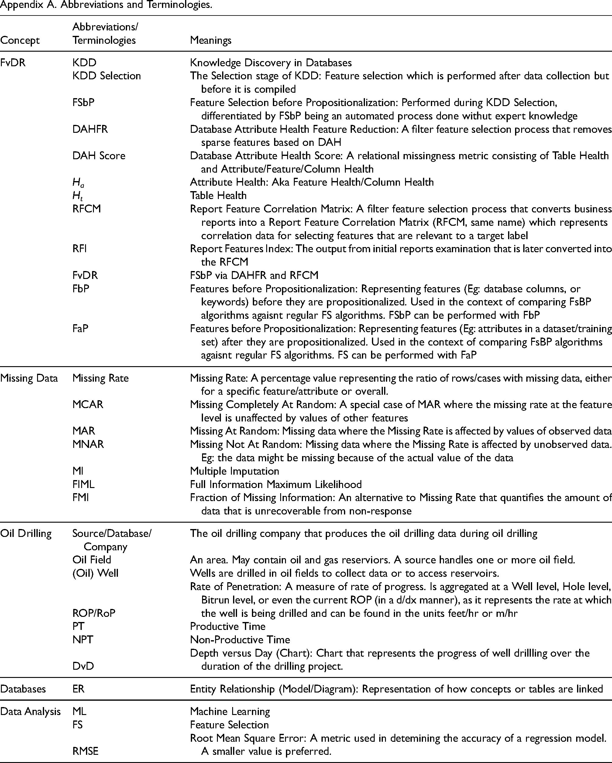
Appendix A. Abbreviations and Terminologies.
| Concept | Abbreviations/Terminologies | Meanings |
|---|---|---|
| FvDR | KDD | Knowledge Discovery in Databases |
| KDD Selection | The Selection stage of KDD: Feature selection which is performed after data collection but before it is compiled | |
| FSbP | Feature Selection before Propositionalization: Performed during KDD Selection, differentiated by FSbP being an automated process done withut expert knowledge | |
| DAHFR | Database Attribute Health Feature Reduction: A filter feature selection process that removes sparse features based on DAH | |
| DAH Score | Database Attribute Health Score: A relational missingness metric consisting of Table Health and Attribute/Feature/Column Health | |
| H a | Attribute Health: Aka Feature Health/Column Health | |
| H t | Table Health | |
| RFCM | Report Feature Correlation Matrix: A filter feature selection process that converts business reports into a Report Feature Correlation Matrix (RFCM, same name) which represents correlation data for selecting features that are relevant to a target label | |
| RFI | Report Features Index: The output from initial reports examination that is later converted into the RFCM | |
| FvDR | FSbP via DAHFR and RFCM | |
| FbP | Features before Propositionalization: Representing features (Eg: database columns, or keywords) before they are propositionalized. Used in the context of comparing FsBP algorithms agaisnt regular FS algorithms. FSbP can be performed with FbP | |
| FaP | Features before Propositionalization: Representing features (Eg: attributes in a dataset/training set) after they are propositionalized. Used in the context of comparing FsBP algorithms agaisnt regular FS algorithms. FS can be performed with FaP | |
| Missing Data | Missing Rate | Missing Rate: A percentage value representing the ratio of rows/cases with missing data, either for a specific feature/attribute or overall. |
| MCAR | Missing Completely At Random: A special case of MAR where the missing rate at the feature level is unaffected by values of other features | |
| MAR | Missing At Random: Missing data where the Missing Rate is affected by values of observed data | |
| MNAR | Missing Not At Random: Missing data where the Missing Rate is affected by unobserved data. Eg: the data might be missing because of the actual value of the data | |
| MI | Multiple Imputation | |
| FIML | Full Information Maximum Likelihood | |
| FMI | Fraction of Missing Information: An alternative to Missing Rate that quantifies the amount of data that is unrecoverable from non-response | |
| Oil Drilling | Source/Database/Company | The oil drilling company that produces the oil drilling data during oil drilling |
| Oil Field | An area. May contain oil and gas reserviors. A source handles one or more oil field. | |
| (Oil) Well | Wells are drilled in oil fields to collect data or to access reservoirs. | |
| ROP/RoP | Rate of Penetration: A measure of rate of progress. Is aggregated at a Well level, Hole level, Bitrun level, or even the current ROP (in a d/dx manner), as it represents the rate at which the well is being drilled and can be found in the units feet/hr or m/hr | |
| PT | Productive Time | |
| NPT | Non-Productive Time | |
| DvD | Depth versus Day (Chart): Chart that represents the progress of well drillling over the duration of the drilling project. | |
| Databases | ER | Entity Relationship (Model/Diagram): Representation of how concepts or tables are linked |
| Data Analysis | ML | Machine Learning |
| FS | Feature Selection | |
| RMSE | Root Mean Square Error: A metric used in detemining the accuracy of a regression model. A smaller value is preferred. |