CSIMFS: An algorithm to tune fuzzy logic controllers

Abstract

This work, presents a new tuning algorithm for type-I fuzzy logic controllers (FLCs), called Change Symmetry in Input Membership Functions (CSIMFS). The algorithm uses an iterative method that applies specific criteria to reduce mathematical operations during the tuning process to develop embedded FLCs. It uses one-input-one-output fuzzy inference system with five control rules and no more than two tuning parameters. The effectiveness of the proposed algorithm was validated experimentally using a real nonlinear pneumatic positioning system and verified with a simulation using a second order model. In both cases, CSIMFS algorithm exhibited a better performance compared with heuristically tuned FLCs. Moreover, a new combined performance index was defined and compared to traditional ITAE index offering better results, reducing the maximum overshoot and a faster convergence of settling time.

Keywords

FLC tuning algorithm fuzzy logic control controller performance indexes nonlinear control

1 Introduction

The fuzzy logic controllers are an alternative for those applications where classical control strategies are not suitable, especially when the dynamical behavior of the plant cannot be modeled mathematically. Those systems with non-linear behavior always require human operator experience to operate. A FLC is suitable in cases when numerous information exists from several variables, a low precision environment, vague information, and also in systems with no predictable disturbances, inherent uncertainties or low accurate sensors [1].

The use of a FLC is often limited, due to inadequate and insufficient methods or non-systematic procedures, for its design and tuning [2, 3]. For this reason, many researchers have tried to improve the FLC tuning methods to make its design easier and faster. A FLC has no fixed structures like conventional PD, PI, and PID controllers. A standard and systematic method for the tuning of FLCs is still under development. There is still no well-defined criteria for deciding on [4]:

The shape of membership functions (MFs)

The number of linguists terms

The standard rule-base

The most appropriate inference mechanism

Fuzzification and defuzzification strategies

Range and grade of symmetry of every input-output MF

Overlap percentage

Number of crossing points in the MFs

Input and output scaling factors

The performance of the FLCs is affected by these diverse criteria, making it difficult to find an optimal. Since pioneering works in the mid 80’s, a wide range of tuning methods has been proposed in the literature. A first approach is based on automatic rule base generation, by using different methods like gradient descent techniques [5, 6], feed-forward neural networks [7, 8], radial basis function networks [9], fuzzy clustering [10, 11] and genetic algorithms [12]. These systems learn to control the process through training. Unfortunately, a finite number of rules must be specified a priori, causing a slow learning rate with a high computational cost.

Another approach is using a combination of automatic modification of input and/or output scaling factors and the initial rule-base definition. Maeda and Murakami [13], proposed a self-tuning algorithm with two main functions: the adjustment of input-output scaling factors as parameters of the FLC and the improving of the control rules by the comparison of the control response with the target response. Daugherity et al. [14], based on Maeda and Murakami work, proposed a simpler technique, adjusting the input scaling factors without modifying the pre-established control rules to get the desired performance.

Furthermore, Jamaludin et al. [15] proposed a self-tuning mechanism to get the adjustment of the input MFs of a FLC. The tuning process was carried out by reshaping the triangles of five input MFs with the compression or expansion of the distance between the vertexes of the triangles along the universe of discourse. Considering that each vertex is equally separated from each other by a length l or changing the location of the middle bound or both.

Rajni Jain et al. [16], proposed a tuning of the MFs and control rules for a FLC using simulated annealing (SA) optimization technique. An improved performance was obtained by minimizing the error function, through adjusting the location of the peak values of the triangular input MFs, moving their base and keeping the shape unchanged. Trung-Kien Dao et al. [17] addressed the tuning problem by parameterizing the input-output MFs of a FLC with scaling factors and deforming coefficients, which could be used as control parameters in the optimization by genetic algorithms. Gomez-Ramirez [18], presented an algorithm for tuning a FLC using only one variable to manipulate the settling time of the system through the modification of the domain of the input MFs with a set of scaling factors.

Hybrid self-tuning controllers are developed using specific techniques. Chao and Teng [19], presented a PD like self-tuning FLC system based on adjusting input-output scaling factors in a two-stage process, resulting in an efficient method for fully compensating the steady-state error without modification of fuzzy logic rules. Similarly, Mudi and Pal [4], proposed a robust self-tuning method for PI and PD type FLCs, which consists in the online adjustment of the output scaling factors by fuzzy rules, according to the current trend of the controlled process.

Different AI (Artificial Intelligence) techniques have been proposed to solve the FLC tuning problem. For instance, Liu et al. [20], developed an adaptive FLC based on the concept of linguistic hedges and genetic algorithms. The linguistic hedge operators were used to dynamically adjust the shape of the system membership functions. The genetic algorithms were adopted to search the optimal hedge combination in the linguistic hedge module. Other approaches which use genetic algorithms are described in [21 –24]. Another AI technique that is widely applied is the use of neural networks [25, 26].

Another issue in a FLC is to deal with the system uncertainties due to noisy signals and truncation errors, affecting the tuning process and performance of the controller. Main uncertainties in experimental results generally come from fluctuations in measurements, either because settings are not exactly reproducible due to imperfections in the equipment, imprecision in observing the procedure, or a combination of both [27].

Considering all described references with their limitations, new approaches are needed to tune FLCs for quick and effective algorithms, especially in nonlinear plants where a mathematical model is not available. In this work, a novel methodology called Change Symmetry in Input Membership Functions (CSIMFS) is proposed, it uses an iterative algorithm to tune a FLC. Its main characteristics are:

Single-Input Single-Output (SISO) Mamdani-type system.

MFs modification occurs only in the input variable.

Five input MFs mapped one to one with five output MFs.

Sequential redefinition of input MFs is made in predefined discrete units.

Based on the comparison between performance indexes, actions are taken to adjust the input MFs.

Use of simple operations in order to be fully compatible with embedded systems [28].

In order to test the proposed tuning methodology, a non-linear pneumatic positioning plant was used, with a dynamics hard to model analytically [29]. The effectiveness of the CSIMFS algorithm applied in pneumatic positioning system was better than a FLC without the tuning algorithm. As a complement, CSIMFS tuning algorithm was tested in a simulation case using a classical plant of second-order adding to this model a type-dead-zone nonlinearity, induced noise and feedback delay time.

2 Experimental physical plant and fuzzy control algorithms

This section describes the experimental physical plant, a general Fuzzy logic controller FLC, the CSIMFS proposed tuning algorithm for FLCs, a new performance index definition, and a description of a simulated controller implementation.

2.1 The experimental physical plant

The nonlinear plant used to validate our CSIMFS tuning algorithm methodology is a closed-loop pneumatic positioning system with a FLC for ball position controller. Its components are illustrated in Fig. 1. A commercial VGA camera is used as visual feedback sensor, capturing RGB type images of the full sphere movement path inside the transparent acrylic tube. A computer vision system as shown in Fig. 4, processes the images with the algorithm coded in ‘C’ language using a Dell™ Laptop with a processor Intel^® Core™ i7-4500U CPU @ 1.80 GHz, installed memory (RAM) of 8.00GB and a 64-bit operating system Windows^® 8 of Microsoft. This program, calculates the distance of the sphere centroid to the base of the tube with less than 2% error.

Fig.1

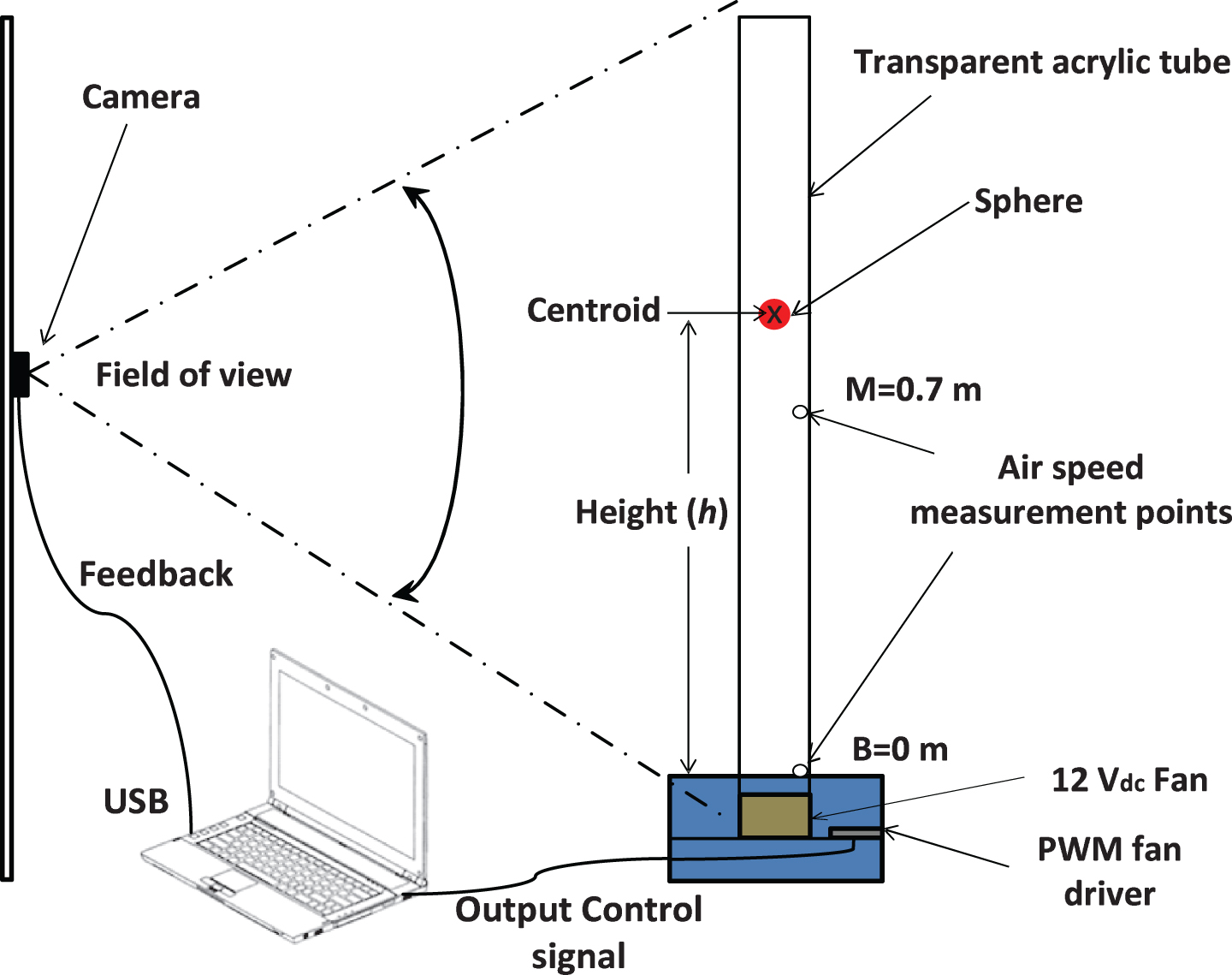
Components of the pneumatic positioning system with a close loop control.

Fig.2

Tracking the height of the sphere inside the tube versus the PWM duty cycle of the fan speed control.

Fig.3

Airflow speed measurements with and without the sphere at B = 0 m and M = 0.7 m.

Fig.4

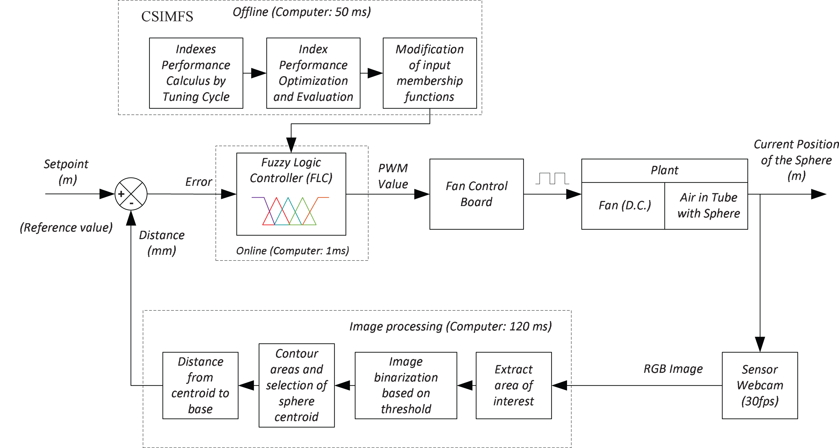
A general block diagram of the system control integrating the CSIMFS tuning algorithm and Image processing block diagram.

The main blocks of the proposed algorithm are shown in Fig. 4, details were published in [30]. The image processing system requires 120 ms to give a height sphere value (h) which is the feedback signal input to the control system. The error magnitude (e) is the difference between the setpoint and calculated height (h), and it is used to define the new fan speed to minimize it.

The transparent acrylic tube has a 1400 mm length with an external diameter of 76.2 mm and an internal diameter of 70.2 mm. A box base made with the same material of the tube has dimensions of 299×248×295 mm. Expanded polystyrene sphere has a diameter of 60 mm and a density of 0.011 g/cm³.

Considering the classical controller design, we selected as input control variable the error (e), and as output variable the sphere position (h), which has a non-linear relationship with the fan speed. The PWM duty cycle range for the fan speed was selected in the [75%, 85%] interval, where 100% is the maximum pulse width and is equivalent to 255 in digital representation. The nonlinear relation between the sphere positions versus the PWM duty cycle for the fan is shown in Fig. 2. Error bars indicate the standard deviation of five measures for every duty cycle increment from 75% to 85%. There is an initial dead zone, which is broken at an 80% duty cycle value. After that, the sphere starts rising within the airflow, presenting an exponential behavior until it reaches the top of the tube at 85% duty cycle. Error increases as height increases due to its incremental random movement related to the height of the sphere.

Air behavior inside the tube, is strongly influenced by the sphere. Air measurements were performed in two particular locations of the tube, at the bottom near to the fan (B = 0 m), and in the middle of the column (M = 0.7 m) as indicated in Fig. 1.

We sampled five times the airflow speed for every duty cycle value using a commercial Lutron™ hot wire anemometer model AM-4204; it has a resolution of 0.1 m/s and an accuracy of±5%. Figure 3, shows the comparison of the airflow speed versus the PWM duty cycle for the fan speed with and without the sphere inside the tube. An almost linear behavior is obtained when the sphere is not inside the tube, changing drastically when the sphere is placed into the tube.

When the sphere is inside the tube, the behavior becomes highly nonlinear in both testing points, presenting high turbulence and unstability in the sphere movement (77– 81% PWM duty cycle). The vertical movement starts at ∼77% PWM duty cycle, and the airflow speed changes at the bottom (B = 0 m), from ∼0.4 m/s to a maximum of ∼1 m/s at a ∼79% duty cycle, presenting a rapid increase profile. Airflow speed in the middle of the tube (M = 0.7 m) is higher than at the base. The maximum airflow reached was ∼1.8 m/s for a ∼78% duty cycle value, presenting also a rapid increase profile.

In summary, the pneumatic positioning system becomes a nonlinear plant when the sphere is introduced inside the tube. There are many variables where one or more of them, might be affecting each other; making difficult to design the controller. Some potential variables that affect the correct positioning of the sphere are:

Mass and density

Acceleration

Airflow speed

Airflow temperature

Drag effect

Rotational motion in the direction of the ‘x’, ‘y’, ‘z’ axes

Translational motion in the direction of the ‘x’, ‘y’ axes

Roughness

Sphericity

Tube diameter

Roughness of the inside wall of the tube

Air pressure distribution around the sphere

Grade of airflow turbulences

With so many factors involved, a mathematical model for describing the system is unmanageable, requiring a fuzzy controller with an adequate tuning algorithm.

2.2 Fuzzy logic controller

A robust alternative for developing controllers for non-linear plants like the one described previously is the integration of unconventional controller types with a model-free control scheme. We applied a SISO Type-I FLC for this case.

Figure 4 illustrates the complete block diagram for the implemented system. It is subdivided in three blocks: the CSIMFS tuning algorithm, the image processing algorithm, and the closed loop FLC algorithm. It works as follows:

The user selects the desired set point for positioning the sphere.

The current sphere position is obtained through a digital camera which sends the digital image to the computer to be processed.

The image processing algorithm is a four stage process [30] in which the first step is to automatically extract the area of interest which comprises the tube with the sphere inside it. Second step is to binarize the image using a color treshold that allow us to identify the red ball in a contrasting scenario (black background: A black vinyl film was adhered to the transparent tube covering half of tube).

Third step is to find a unique point which represents the centroid of the sphere by locating the contour of the sphere and calculating its center. Finally, using the centroid of the sphere, the distance to the base is calculated to obtain a unique integer representing the position h.

The error e is calculated and introduced into the FLC, which obtains the control action to modify the current fan speed by means of PWM. This signal is electronically amplified in the fan control board, converting it into a DC signal able to operate the fan.

The closed loop control leads us to step 2 continously, pushing the sphere to the desired height by increasing or decreasing the fan speed according to FLC output. This actions loops until the user stops the system.

The integration of steps 1– 5 in a fuzzy control system for the physical plant described previously (Section 2.1) in a comparative study with conventional controllers PD, PI and PID was published in 2014 [29].

The CSIMFS tuning algorithm is trained offline by adjusting the current FLC parameters to find an optimum, following the procedure explained in the next section.

2.3 CSIMFS tuning algorithm for fuzzy controllers

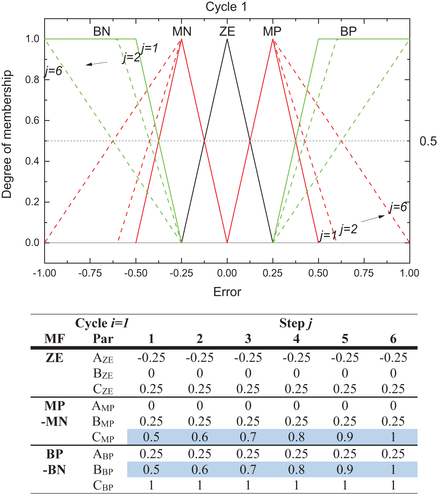
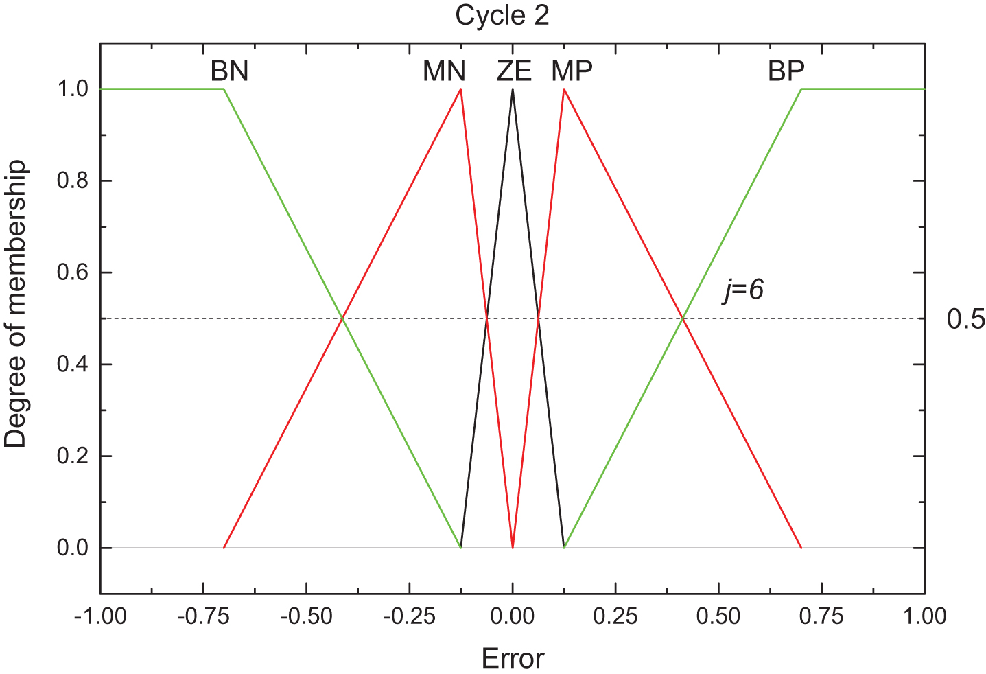
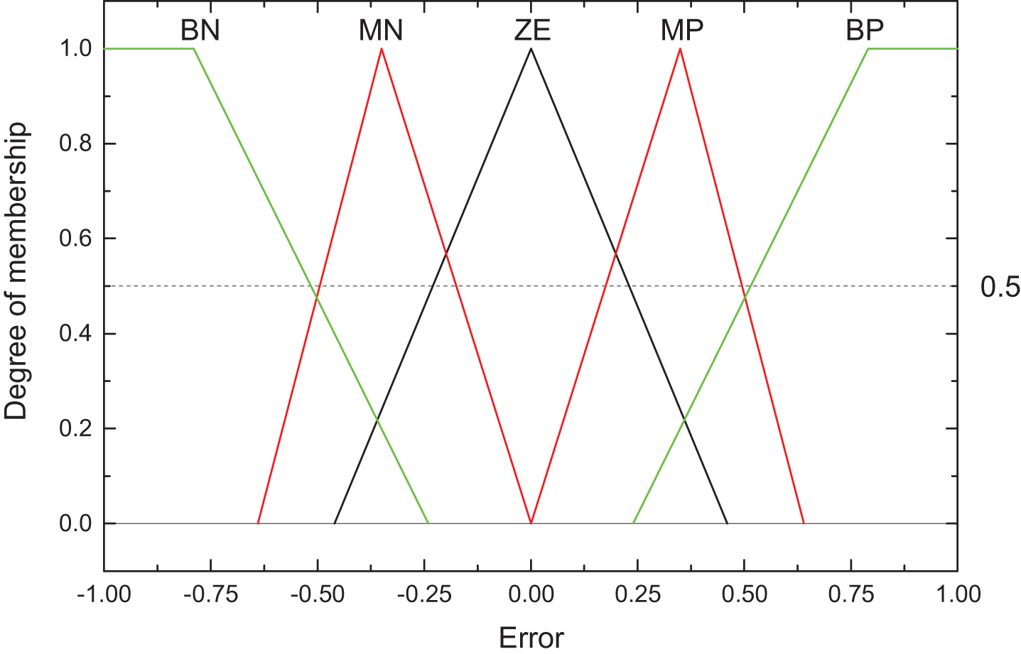
General FLCs tend to have an excessive number of parameters to configure and select appropriately (tuning process), affecting the final response of the controller. Conversely, the CSIMFS (Change Symmetry of Input Membership Functions) tuning algorithm proposed for embedded FLCs, works with only two parameters and it is described as follows:

The linguistic terms used to name each membership function at input (Error) and output (PWMdutycycle) fuzzy sets are shown in the table of Fig. 5. The distribution of the MFs is with three central triangular MFs and two trapezoidal MFs in the boundaries. Main parameters for CSIMFS algorithm, that define the shape of their triangular MFs and trapezoidal MFs are labeled over the ‘x’ axis. The input universe [– 1.4, 1.4] m was normalized to the range [– 1, 1] and the output universe [0, 100%] PWM duty cycle, was normalized to the range [0, 1]. The Mamdani fuzzy inference and centroid defuzzification methods were used. Five fuzzy rules are defined as a one to one relation, as shown in data table of Fig. 5, these are:

If <Error is BN>then <PWM is S>

If <Error is MN>then <PWM is MS>

If <Error is ZE>then <PWM is M>

If <Error is MP>then <PWM is MF>

If <Error is BP>then <PWM is F>

The input variable modification consists in changing the symmetry of the MFs that are adjacent to the central one in an step process. This is achieved by increasing to the sides, the domain of each triangular MFs on the left and right side of the central one as in Fig. 6.

The initial right boundary value of the right triangular MF next to the central MF, which comes from previous definition at the ith cycle, it is consecutively increased in 0.1 steps until it reaches +1. Symmetrically, the left boundary value of the central MF, is decreased in – 0.1 steps until reaching – 1.

The initial cycle (i = 1) begins with the positive values of C_MP = 0.5 = B_BP, which change in 0.1 steps until C_MP = 1 = B_BP. The same happens in the negative side at points B_BN and A_MN. This parameters change by steps as shown in Fig. 6.

The domain of lateral trapezoidal MFs changes its position in order to maintain the adjacent crosspoints at 0.5 value.

The consecutive redefinition at the beginning of every tuning cycle (i> 1) consists of reducing to the half the domain of the triangular MFs as illustrated in Fig. 7.

The performance analysis and tuning can be made using any of the following performance indexes: Integral Time Absolute Error (ITAE), Square Error (ISE), Maximum Overshoot percentage (% MOS), Rise Time (T_r), and Settling Time (T_s). A new combined index is proposed to improve the performance, it includes % MOS, T_r, and T_s, it was named % ZI and it is formally defined in Section 2.4.

The search of optimal parameters for the FLC, is performed in every tuning cycle. It computes all performance indexes for every step j in the cycle i. The algorithm obtains the minimum index value from the selected ones for all the iterations in the current tuning cycle.

It is necessary to complete at least two tuning cycles to compare.

If the minimum index value in the current i tuning cycle is greater than the obtained value in the previous i-1 cycle, the tuning process ends. Otherwise, the process continues with another tuning cycle. Table 1, shows the evolution of the performance indexes for the second tuning cycle where the minimum value for % ZI is found in iteration (i = 2, j = 6) and the minimum ITAE and ISE value in iteration (i = 2, j = 8) were found. These indexes were compared with the values obtained in tuning cycles 1 and 3 and the algorithm finished here because the stopping criteria was satisfied.

According with the results shown in Table 1, the tuned parameters to define the input MFs which were selected by the CSIMFS algorithm at iteration (i = 2, j = 6), are represented by the vectors (1– 5). The resulting shape is illustrated in Fig. 8.

Fig.5

The initial definition for membership functions of: a) Input universe, b) Output universe and linguistic terms used to name input- output MFs are summarized at bottom.

Fig.6

Graphs of MFs and their parameter evolution as function of iteration for cycle i = 1. Left side MFs parameters are symmetric with same values but negative. MFs are plotted for three steps values highlighted (j = 1, j = 2 and j = 6). Raws highlighted indicates the values of the parameters that changes in every step.

Fig.7

Graphs of MFs and their parameter evolution as function of iteration for cycle i = 2. Left side MFs parameters are symmetric with same values but negative. MFs are plotted for three step values highlighted (j = 1, j = 3 and j = 9).

Table 1

The numeric evolution of the performance indexes for the tuning cycle 2

Iteration 2, j	ITAE	ISE	% MOS	Tr(s)	Ts(s)	% ZI
1	106.7	35.5	24.7	3.2	44.0	36.9
2	90.2	25.1	22.3	3.1	38.0	32.6
3	90.1	25.4	23.7	3.1	44.1	36.4
4	98.5	30.3	26.5	2.7	47.2	39.3
5	100.7	30.6	22.8	3.2	48.3	38.3
6	90.4	25.5	12.1	3.6	29.7	23.4
7	107.9	36.3	19.9	3.1	47.7	36.4
8	73.9	16.7	19.0	3.2	38.0	30.9
9	85.8	22.3	18.0	3.1	48.4	35.8

Fig.8

Tuned definition of MFs for the input error as result of applying CSIMFS algorithm, where cycle i = 2, step j = 6 produced best results.

BN = [- 1, - 1, - 0.7, - 0.125]

(1)

MN = [- 0.7, - 0.125, 0]

(2)

ZE = [- 0.125, 0, 0.125]

(3)

MP = [0, 0.125, 0.7]

(4)

BP = [0.125, 0.7, 1, 1]

(5)

Although in the experimental validation of CSIMFS tuning algorithm we selected the ITAE index as our first approach, since the time appears as a factor, it will penalize errors that occur late in time, even though it practically ignores the errors that occur in early time. This produces the largest percent overshoot (% MOS), but it will give us the shortest settling time [31]. As a potential solution to attend this problem, a new mixed index is proposed in this work named % ZI. It is a function of rise time (T_r), settling time (T_s) and % MOS, to reduce the maximum overshoot equilibrating and maintaining in appropriate values the rise time and the settling time. It is defined in the next section.

2.4 The % ZI as composed performance index

If the initial overshoot is critical in the operation of specific equipment and systems, we need to choose between selecting another control strategy for overshoot cushioning or selecting a new performance index that focuses on reducing the maximum overshoot with a finite settling time during the tuning process. After a qualitative analysis, we noticed that there is not a known performance index, which guarantees to achieve these characteristics. Hence, it is proposed a new one.

As the amplitude of the maximum overshoot is related to the rise time (T_r) and the settling time (T_s), a composed performance index is proposed considering contributions from the three most critical indexes with an experimental weight factor: the MOS with a 50% weight; T_s and T_r, both with a 25% weight. Those values were selected after different experiments due to the good results obtained. The greatest weight was given to the % MOS, as it is critical for reaching the settling time (T_s) in short time with good response time (T_r), in a stable control system. According with Table 1, the ITAE and ISE indexes do not guarantee a minimum value for % MOS neither a minimum settling time (T_s). The % ZI index guarantees minimum values for % MOS and T_s and slightly major rising time (only 25%) than the minimum value found (iteration 2, 4).

The settling time (T_s) and rise time (T_r) are divided by the total response time T in order to obtain their relative magnitude in percentage. The new performance index is named % ZI and is expressed by the following Equation (6):

$\begin{matrix} % ZI & = & (0.25) (\frac{T_{r}}{T}) (100) + (0.5) (% MOS) \\ + (0.25) (\frac{T_{s}}{T}) (100) \end{matrix}$ (6)

2.5 Simulation case

To illustrate the impact of the proposed CSIMFS tuning methodology, a comparison in a simulation scenario was performed with a classical model for a DC motor, defined with a second order model. The transfer function between the motor displacement (θ_m (s)) and the input voltage (E_a (s)) is given by Equation (7) obtained in reference [32], $\frac{θ_{m} (s)}{E_{a} (s)} = \frac{K_{t}}{L_{a} J_{m} s^{3} + (R_{a} J_{m} + B_{m} L_{a}) s^{2} + (K_{b} K_{t} + R_{a} B_{m}) s}$ (7)

Where the motor parameters are defined as follows:

K_t= torque constant (Nm/A),

K_b= back-emf constant (Vs/rad),

L_a= armature inductance (H),

R_a= armature resistance (Ω),

J_m= rotor inertia (Kgm²),

B_m= viscous-friction coefficient (Nms),

The relation between angular position θ_m (s) rad and angular speed ω_m (s) rad/s is: $θ_{m} (s) = \frac{1}{s} ω_{m} (s)$ (8)

Then substituting the Equation (8) into the Equation (7), it is obtained the relation between rotor shaft speed and applied armature voltage being a second order model represented with the transfer function: $\frac{ω_{m} (s)}{E_{a} (s)} = \frac{K_{t}}{L_{a} J_{m} s^{2} + (R_{a} J_{m} + B_{m} L_{a}) s + (K_{b} K_{t} + R_{a} B_{m})}$ (9)

Several works have been published in relation to the use of this model proposing parameters for a DC motor and conventional control techniques and in combination with artificial intelligence techniques [33 –37]. We choose the DC motor number 1 parameters, proposed by Meshram et al. [35]. They use 3 different DC motors models through simulation to validate a modified Ziegler-Nichols PID tuning technique. It was selected this DC motor parameters, due to the lowest torque constant with a value of 0.015 Nm/A. This small value is adequate for a small motor with small-load and high-speed application; our DC motor is small with an input power of 2.52 W, no-load in a fan application, maximum speed of 3250 R.P.M. and maximum airflow of 1.06 m³/min. The part number is AUB0812HH™ of Delta Electronics, Inc.

Substituting the parameters selected (K_t= 0.015 Nm/A, K_b= 0.01 Vs/rad, R_a= 2Ω, J_m= 0.02 Kgm², L_a= 0.5 H and B_m= 0.2 Nms) in Equation (9), is obtained the transfer function: $G (s) = \frac{ω_{m} (s)}{E_{a} (s)} = \frac{0.015}{0.01 s^{2} + 0.14 s + 0.40015}$ (10)

This model also represents a system commonly found in many real-world applications as a mass-spring-damper system. An exponential term was added with a factor of 2.5 to consider the average delay time to start the sphere movement upward. Then, Equation (10) becomes $G (s) = \frac{(0.015) (e^{- 2.5 s})}{0.01 s^{2} + 0.14 s + 0.40015}$ (11)

Next modifications were added in the model to increase its similarity with the physical plant. a) A delay block of 0.120 s is included in the feedback loop to consider the image processing delay, b) A constant noise signal with a sample time of 0.01 s, with a maximum value of 0.025, to consider the inherent error of the measurement system of processing image unit (minor than 2%), and c) Communication delays between software and hardware.

3 Results and discussion

This section presents the response results of a FLC and its improvement by the use of CSIMFS tuning algorithm and the % ZI performance index.

To probe the efficiency of the CSIMFS tuning algorithm, the experiments were performed using three different controllers with the same initial conditions. The first one is a heuristically tuned FLC by trial and error (subsection 3.1), the second is a CSIMFS tuned controller (subsection 3.2), and the third is a simulated CSIMFS (subsection 3.3). The set point for the three controllers is at the middle of the column h = 0.7 m, since we have demonstrated from Fig. 3 that is a nonlinear section of the plant. All controllers, use qualitatively the same number of initial membership functions with the same distribution, as in Fig. 5.

Last subsections contain a general discussion and stability issues.

3.1 Heuristically tuned fuzzy logic controller

Two FLCs tuned without the CSIMFS tuning algorithm were selected to compare its response time with the one that uses the proposed tuning algorithm. FLC tuned with the initial input-output MFs showed in Fig. 1, is labeled FLC Initial. Its response is shown in Fig. 9, which also illustrates the response of a FLC tuned heuristically, labeled FLC Heuristic. This corresponds to a tuned FLC through relating the change of the symmetry of membership functions laterals next to the central, in the input universe with the change of the slope of the central region of the control surface and its corresponding response over time.

Fig.9

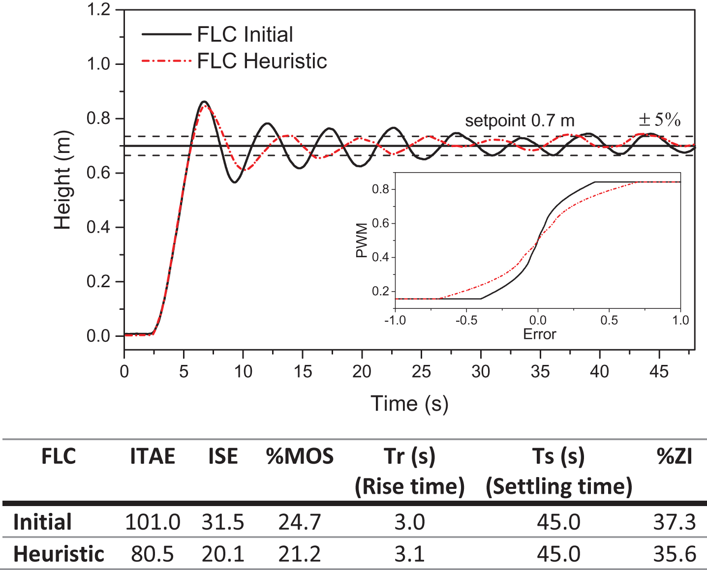
Graphs of the FLC Initial response with the initial definition of input MFs and FLC Heuristic with an additional heuristic adjustment. An inset with correspondent control curves is included.

The slope of the flat region of the control curves (inset in Fig. 9) has a direct relationship with the speed response of the system and its settling time, as well as, with expansion or compression of the MF in the center and the MFs aside of it [3]. The slope of the central region of the control curve of FLC Heuristic is lower than FLC Initial, with slower reaction to small errors and input changes so, it has lower sensitivity. This corresponds to a wider domain in the central MF and reduced domain in the lateral MFs. In contrast, the slope of the central region of the control curve of FLC Initial is higher, with a fast reaction to small errors and input changes so, it has a high sensitivity. This corresponds to a reduced domain in the central MF and the same or wider domain in the lateral MFs.

Amplitude of the oscillations around the setpoint in the FLC Initial, are bigger than the amplitude of the oscillations in the FLC Heuristic. The percent of maximum overshoot is slightly bigger in the FLC Initial response. According to the numerical values of the performance indexes, there was an overall performance improvement with the FLC Heuristic response (the final definition of input MFs for the FLC Heuristic, is shown in Fig. 10). For instance, the ITAE index decreased its value in 20.3%, the percent of maximum overshoot (% MOS) decreased in 14.1%. The % ZI decreased only 4.5% due to the integrating parameters % MOS, T_r and T_s slightly changed.

Fig.10

The final definition of input MFs of the FLC Heuristically tuned.

3.2 Fuzzy logic controller with the CSIMFS tuning algorithm

Applying the proposed CSIMFS tuning methodology to the same FLC, we obtained the responses illustrated in Fig. 11, which shows the best responses for the second (i = 2), and third (i = 3) tuning cycles. Each graph represents the best % ZI performance for a specific iteration (i, j). In the first tuning cycle (i = 1), the % ZI does not converge, and the algorithmdiscriminates all responses of every iteration.

Fig.11

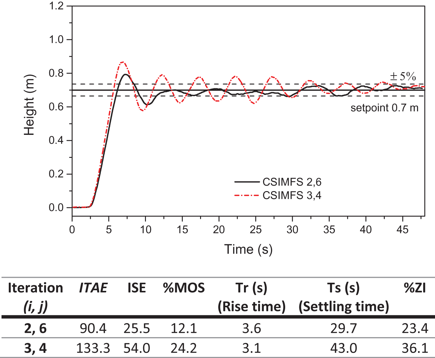
The tuning process through % ZI index, applying the proposed algorithm, showing for each of two tuning cycles the best response in iteration (i j) and their performance indexes.

The data table in Fig. 11, summarizes the performance indexes for every response. At iteration (2, 6), the minimum value for the % ZI was obtained contrasting with the second and third cycle. The tuning process finishes here because the minimum % ZI value obtained in third cycle for iteration (3, 4) is greater than the minimum % ZI value obtained in second cycle for iteration (2, 6). Example used in CSIMFS description (Fig. 8), shows the final definition of the input MFs for iteration (2, 6).

As important note, the output membership functions did not change during all tuning process.

3.3 Simulation case

According to the model proposed for a DC motor represented by Equation (11), using SIMULINK™ of MATLAB R2014a and applying the CSIMFS algorithm with the % ZI, ITAE and ISE indexes we obtained the step responses of the system, and they are shown in Fig. 12.

Fig.12

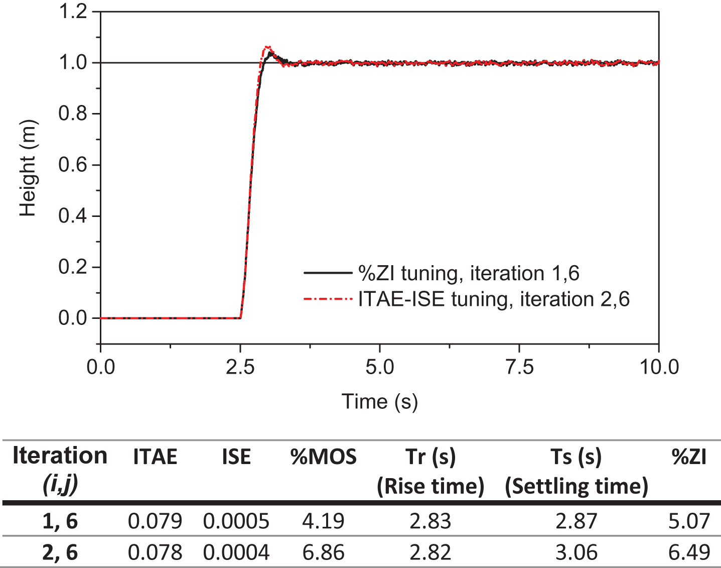
Comparison between simulated responses of the CSIMFS tuned fuzzy control system using the ITAE, ISE and % ZI performance indexes.

The minimum value for % ZI was found in iteration (1, 6), the minimum values for ITAE and ISE indexes matches in iteration (2, 6).

3.4 Discussion

Looking at Figs. 9 and 11, once the system reaches the settling time with a relative error of less than 5%, the system presents oscillations around the set point due mainly to time delay in the feedback signal originated by the image processing unit and time delays of communication between hardware and software.

A FLC with high sensitivity produces a big overshoot with an increase in settling time (due to, wider oscillations at the end of the response). In contrast, a FLC with a low sensitivity produces a smaller overshoot with narrower oscillations at the end of the response but is slower to reach the set point. The CSIMFS tuning algorithm found the best input MFs parameters for the proposed FLC, this occurs in iteration (2, 6) with the lowest % ZI index in the experimental physical plant.

According to the previous controller responses, we compared the best two controllers in Fig. 13. For the FLC Initial and the heuristically tuned FLC, this corresponds to the tagged as FLC Heuristic, and for the best FLC tuned by the CSIMFS tuning algorithm corresponds to FLC (2, 6). The performance indexes for every response are located below the graph. The CSIMFS tuned FLC (2, 6), presented a substantial performance improvement over the heuristic controller.

Fig.13

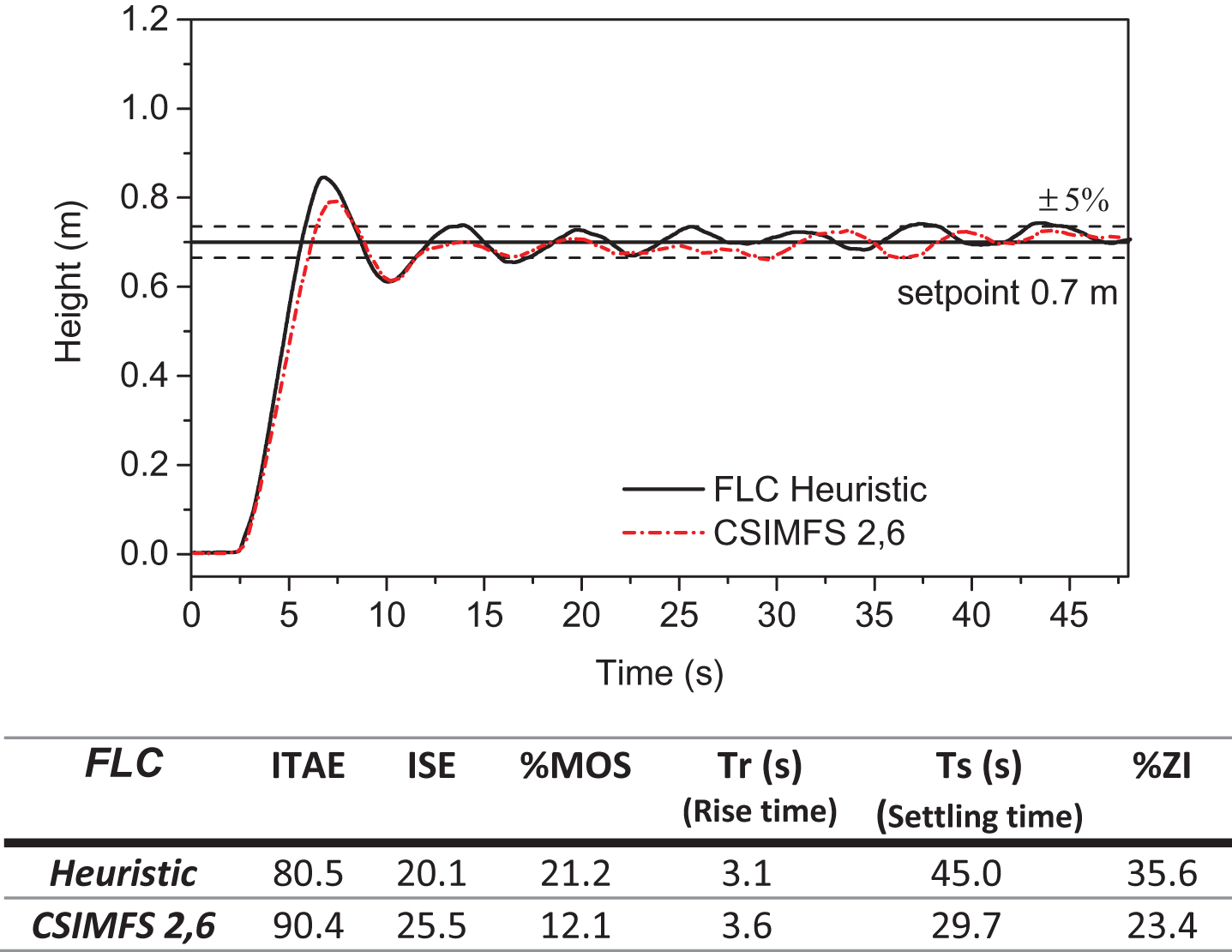
Comparison between system responses with the FLC Heuristic tuned, and the FLC tuned with the CSIMFS algorithm.

The table in Fig. 13, shows that settling time was reduced up to 34% and the percent of maximum overshoot (% MOS) decreased by 42.9%. The % ZI also improved, although there was a slight increase in the rise time. In contrast, the ITAE increased its value in 12.3% and the ISE in 26.8%.

The ITAE index is not sensitive to the initial error in the transient period causing a big overshoot. Because of this, we also selected the % ZI index, and the system found that after the first tuning cycle, the best value was found at step 6, as shown in Figs. 11–13.

By applying the CSIMFS tuning methodology and using the new % ZI performance index, we obtained an acceptable response with fewer operations in only two tuning cycles. In contrast, when using the ITAE or ISE indexes for tuning, it required three tuning cycles.

In the simulation case, the minimum values of ITAE, ISE and % ZI indexes are shown in Table 2, for the first three consecutive tuning cycles.

Table 2

The numeric behavior of the ITAE, ISE and % ZI indexes for the first 3 tuning cycles of the proposed CSIMFS tuning algorithm for the simulation case

Tuning cycle	ITAE	ISE	% ZI
1	0.079	0.0005	5.07
2	0.078	0.0004	6.24
3	0.082	0.0005	6.40

This performance contrasts with other works that required three steps for scaling factors adjustment and ten steps for rule modification [13], and thirteen tuning steps with the scale factors initialized to the unity under the same selected indexes [14].

3.5 On the stability issue for the CSIMFS

Stability analysis is very important to guarantee the functionality of nonlinear systems tuned by means of fuzzy controllers. The main problem is that majority of fuzzy models in the reported papers are used for empirically mimicking measured input– output data of the physical systems. There is a variety of stability analysis methodologies in literature [38]. Some methodologies are based in linear matrix problem solving [39], but most of them use the Lyapunov stability theorem for linear systems [40, 41]. The main disadvantage in these methods is their limitation to find an accurate mathematical model of the fuzzy controller as it is naturally nonlinear, resulting that linear control theory cannot be applied [42]. To overcome this difficulties there are other proposals which use stabilization of dynamical systems, dedicated to find the equilibrium point in terms of initial value problems [43, 44].

When referring to the stability analysis of the proposed CSIMFS tuning methodology, any of the mentioned stability approaches can be applied, but it requires an extensive analysis out of the extent of this paper and is considered as future work. For this case, the acknowledgement of the nonlinear plant is used to reduce the affectation of the perturbations in a heuristic form, since the experimental work and the experience about this pneumatic system have helped us to get the stability. By now, we can support that the proposed methodology is stable by the sufficiency condition of presenting an asymptotically stable behavior to an equilibrium point as in [42 , 46]. This behavior can be observed in the reduction of the value of the % ZI index as the iterative process reaches an optimal value which leads us to stop the tuning process.

As future research, it is recommended to analyze the behavior of the proposed CSIMFS tuning algorithm under induced physical disturbances in the pneumatic positioning system for different setpoints. In addition, it is required to probe the proposed tuning algorithm in another kind of physical plants with SISO and MIMO type topologies. Finally, to improve the response of the tuned FLC, it requires a faster feedback measurement system.

4 Conclusion

A new algorithm called CSIMFS to tune type-I SISO Mamdani FLCs is proposed and tested in a physical plant, based in a process of changing the symmetry of input MFs. As a result of applying this new tuning algorithm in the pneumatic positioning plant, a better performance is obtained, improving the settling time and the maximum overshoot percentages in 34% and 43% respectively, regarding a FLC tuned heuristically without the proposed tuning algorithm. These results were obtained in only three tuning cycles.

We used a second-order plant model to test the CSIMFS tuning algorithm in a simulation environment. It also presented a good performance in only two tuning cycles.

A new % ZI performance index was introduced, which integrates into one index, three critical performance metrics for control system response. A faster convergence was obtained to a stable response, discriminating cases of non-success. Consequently, the operations and computational time are reduced as is required for embedded systems.

The use of CSIMFS algorithm with the % ZI index, ensures a much lower overshoot and settling time, and without losing the speed response, to some extent better than using ITAE or ISE indexes.

Footnotes

Acknowledgments

Authors would like to thank the Instituto Politécnico Nacional and CONACYT for their financial support to realize this work.

References

Cordón

, Herrera

and Perergrín

, A practical study on the implementation of fuzzy logic controllers, Int J Intell Control Syst 3 (1999), 1–26.

Haber

, Mario

, Godoy

and Gajate

, Intelligent tuning of fuzzy controllers by learning and optimization, in Fuzzy Modelling and Control: Theory and Applications, Part II, Vol. 9, Matía

, Marichal

, Jimenez

, Eds. Paris: Atlantis Press, 2014, pp. 135–158. doi: 10.2991/978-94-6239-082-9

Shaw

I.S.

, Fuzzy Control of Industrial Systems Theory and Applications, Springer Science+Business Media, LLC, 2013.

Mudi

R.K.

and Pal

N.R.

, A robust self-tuning scheme for PI and PD-type fuzzy controllers, IEEE Trans Fuzzy Syst 7 (1999), 2–16.

Nomura

, Hayashi

and Wakami

, A learning method of fuzzy inference rules by Descent Method, in IEEE International Conference on Fuzzy Systems, San Diego, CA, 1992, pp. 203–210. doi: 10.1109/FUZZY.1992.258618

Hsu

, Hsu

J.Y.

and Chiang

, Automatic Generation of Fuzzy Control Rules by Machine Learning Methods, in IEEE International Conference on Robotics and Automation, Vol. I, 1995, pp. 287–292.

Wang

L.-X.

and Mendel

J.M.

, Generating fuzzy rules by learning from examples, IEEE Trans Syst Man Cybern 22 (1992), 1414–1427.

Pranevicius

, Kraujalis

, Budnikas

and Pilkauskas

, Fuzzy Rule Base Generation Using Discretization, In Dregvaite

, Damasevicius

, Eds., Information and Software Technologies. ICIST 2014. Communications in Computer and Information Science, Vol. 465. Springer, 2014, pp. 160–171.

Cho

K.B.

and Wang

B.H.

, Radial basis function based adaptive fuzzy systems and their applications to system identification and prediction, Fuzzy Sets Syst 83 (1996), 325–339.

10.

Chen

M.-Y.

and Linkens

D.A.

, Rule-base self-generation and simplification for data-driven fuzzy models, in 10th IEEE International Conference on Fuzzy Systems, Melbourne, 2001, pp. 424–427. doi: 10.1109/FUZZ.2001.1007339

11.

Priyono

, Ridwan

and Alias

, Generation of fuzzy rules with subtractive clustering, J Teknol 43 (2005), 143–153.

12.

Ishibuchi

, Nozaki

, Yamamoto

and Tanaka

, Selecting fuzzy if-then rules for classification problems using genetic algorithms, IEEE Trans Fuzzy Syst 3 (1995), 260–270. doi: 10.1109/91.413232

13.

Maeda

and Murakami

, A self-tuning fuzzy controller, Fuzzy Sets Syst 51 (1992), 29–40. doi: 10.1016/0165-0114(92)90073-D

14.

Daugherity

W.C.

, Rathakrishnan

and Yen

, Performance evaluation of a self-tuning fuzzy controller, IEEE International Conference on Fuzzy Systems, 1992, pp. 389–397. doi: 10.1109/FUZZY.1992.258646

15.

Jamaludin

J.Ã.

, Rahim

N.A.

and Hew

W.P.

, Development of a self-tuning fuzzy logic controller for intelligent control of elevator systems, Eng Appl Artif Intell 22 (2009), 1167–1178. doi: 10.1016/j.engappai.2009.04.006

16.

Jain

, Sivakumaran

and Radhakrishnan

T.K.

, Design of self tuning fuzzy controllers for nonlinear systems, Expert Syst Appl 38 (2011), 4466–4476. doi: 10.1016/j.eswa.2010.09.118

17.

Dao

, Chen

, Tuning Fuzzy-Logic Controllers in: Dadios

E.P.

(Ed.), Fuzzy Log - Control Concepts, Theor Appl, 1st ed., INTECH Open Access Publisher 2012, p. 428. doi: 10.5772-2662

18.

Gómez-Ramírez

, Simple tuning of fuzzy controllers, in: Castillo

, Melin

, Kacprzyk

and Pedrycz

(Eds.), Hybrid Intell Syst, Springer Berlin Heidelberg, 2007, pp. 115–133. doi: 10.1007/978-3-540-37421-3_7

19.

Chao

and Teng

, A PD-like self-tuning fuzzy controller without steady-state error, Fuzzy Sets Syst 87 (1997), 141–154.

20.

Liu

B.-D.

, Chen

C.-Y.

and Tsao

J.-Y.

, Design of adaptive fuzzy logic controller based on linguistic-hedge concepts and genetic algorithms, Syst Man, Cybern Part B Cybern IEEE Trans 31 (2001), 32–53.

21.

Bonissone

P.P.

, Khedkar

P.S.

and Chen

, Genetic algorithms for automated tuning of fuzzy controllers: A transportation application, Proc IEEE 5th Int Fuzzy Syst 1 (1996), 674–680. doi: 10.1109/FUZZY.1996.551819

22.

Herrera

, Lozano

and Verdegay

J.L.

, Tuning fuzzy logic controllers by genetic algorithms, Int J Approx Reason 12 (1995), 299–315. doi: 10.1016/0888-613X(94)00033-Y

23.

Homaifar

and McCormick

, Simultaneous design of membership functions and rule sets for fuzzy controllers using genetic algorithms, IEEE Trans Fuzzy Syst 3 (1995), 129–139. doi: 10.1109/91.388168

24.

Cordón

, Herrera

and Lozano

, A Three-stage method for designing genetic fuzzy systems by learning from examples. In Voigt

H.M.

, Ebeling

, Rechenberg

, Schwefel

H.P.

, Eds. Parallel Problem Solving from Nature, Lecture Notes in Computer Science, Vol. 1141, Springer, Berlin, 1996. doi: 10.1007/3-540-61723-X_1035

25.

Lin

C.-T.

and Lee

C.S.G.

, Neural-network-based fuzzy logic control and decision system, IEEE Trans Comput 40 (1991), 1320–1336. doi: 10.1109/12.106218

26.

Abraham

, Adaptation of fuzzy inference system using neural learning, Fuzzy Syst Eng 83 (2005), 53–83. doi: 10.1007/b102051

27.

Bevington

P.R.

and Robinson

D.K.

, Data Reduction and Error Analysis for the Physical Sciences, Third Edition, McGraw-Hill Education, 2003. 336 pages.

28.

Zavala

A.H.

and Nieto

O.C.

, Fuzzy hardware: A retrospective and analysis, IEEE Trans Fuzzy Syst 20 (2012), 623–635. doi: 10.1109/TFUZZ.2011.2181179

29.

Rodríguez Zalapa

, Hernández Zavala

and Huerta Ruelas

J.A.

, Fuzzy Controller for a Pneumatic Positioning Nonlinear System, in: Nature-Inspired Comput Mach Learn, Springer International Publishing, 2014, pp. 370–381.

30.

Rodríguez Zalapa

, Hernández Zavala

and Huerta Ruelas

J.A.

, Distance measurement system using images to determine the position of a sphere using the XBOX kinect sensor, Polibits 1 (2014), 59–67.

31.

Castillo

and Melin

, A review on interval type-2 fuzzy logic applications in intelligent control, Inf Sci (Ny) 279 (2014), 615–631. doi: 10.1016/j.ins.2014.04.015

32.

Kuo

B.C.

and Golnaraghi

, Automatic Control Systems, 9th ed., John Wiley & Sons, Inc., 2010.

33.

Shahgholian

and Shafaghi

, State space modeling and eigenvalue analysis of the permanent magnet DC motor drive system, in 2nd International Conference on Electronic Computer Technology, Kuala Lumpur, 2010, pp. 63–67. doi: 10.1109/ICECTECH.2010.5479987

34.

Moussavi

S.Z.

, Alasvandi

and Javadi

, Speed control of permanent magnet DC motor by using combination of adaptive controller and fuzzy controller, Int J Comput Appl 52 (2012), 11–15. doi: 10.5120/8316-1774

35.

Meshram

P.M.

and Kanojiya

R.G.

, Tuning of PID controller using Ziegler-Nichols method for speed control of DC motor, IEEE-International Conference On Advances In Engineering, Science And Management, Nagapattinam, Tamil Nadu, 2012, pp. 117–122.

36.

Akhilesh Kumar

, Khanna

Navin Kumar

and Vivek

M.K.

, Speed control of DC motor using artificial bee colony optimization technique, Univers J Electr Electron Eng 1 (2013), 68–75. doi: 10.13189/ujeee.2013.010302

37.

Shravan Kumar

, DC motor position control using fuzzy proportional-derivative controllers with different defuzzification methods, IOSR J Electr Electron Eng 10 (2015), 37–47. doi: 10.9790/1676-10133747

38.

M.J.

and Mandal

, A Survey of Adaptive Fuzzy Controllers: Nonlinearities and Classifications, in IEEE Transactions on Fuzzy Systems, vol. 24, no. 5, pp. 1095–1107, Oct. 2016. doi: 10.1109/TFUZZ.2015.2501439

39.

Wang

H.H.O.

, Tanaka

and Griffin

M.F.M.F.

, An approach to fuzzy control of nonlinear systems: Stability and design issues, IEEE Trans Fuzzy Syst 4 (1996), 14–23. doi: 10.1109/91.481841

40.

Feng

, Cao

S.G.

, Rees

N.W.

and Chak

C.K.

, Design of fuzzy control systems with guaranteed stability, Fuzzy Sets Syst 85 (1997), 1–10. doi: 10.1016/0165-0114(95)00375-4

41.

Zadeh

L.A.

, The information principle, Inf Sci (Ny) 294 (2015), 540–549. doi: 10.1016/j.ins.2014.09.026

42.

Kandel

, Luo

and Zhang

Y.Q.

, Stability analysis of fuzzy control systems, Fuzzy Sets Syst 105 (1999), 33–48.

43.

Mizukoshi

, Stability of fuzzy dynamic systems, Int J Uncertainty, Fuzziness Knowledge-Based Syst 17 (2009), 69–83. doi: 10.1142/S0218488509005747

44.

Cecconello

M.S.

, Bassanezi

R.C.

, Brandão

A.J.V.

and Leite

, On the stability of fuzzy dynamical systems, Fuzzy Sets Syst 248 (2014), 106–121. doi: 10.1016/j.fss.2013.12.009

45.

Ashtiani

A.A.

, Nikravesh

S.K.Y.

, Relational Model of Dynamic Systems 9 (2012), 39–48.

46.

Patyra

M.J.

and Mlynek

D.M.

, Fuzzy logic: Implementation and applications, John Wiley & Sons, Inc., 1996.