Prices and order quantities of substitutable products in an EPQ model over different uncertain finite budget constraints

Abstract

In current scenario, big departmental stores used to work more efficiently with the items that can be substituted either with optimum order quantities or selling prices of the products. In this paper, the models are determined as the total profit maximization problem with uncertain finite budget fuzzy constraints thereby solved through a gradient based search technique- GRG (Generalized Reduced Gradient) method. The prices and optimal order quantities of substitutable items are obtained so that total profit for store owner is maximum.

Keywords

Selling price optimal order quantities substitution inventory problems profit EPQ model finite budget constraint

1 Introduction

Inventories are the essential thing needed on most of the places [9]. The function of inventory is inimitable if it passes through the channel of producer to distributor and then finally to a customer. But the absence of inventory shows a tragic moment for customers as far as future profit is concerned. When product becomes out of stock the behavior of customer changes henceforth the following situation arises; a customer may steps aside from that shop and move to some other place or he may wait for item or he may take similar product from the store itself. The phenomenon in the third case is known as product substitution [11]. In a nutshell it depicts how inventory of product will not only effect the demand but also the demand of other products.

Further, Chang [4] calculated the optimal cycle time, optimal reorder time and minimum cost of the EOQ and EPQ models without using classical optimization techniques. Further, Teng et al. [33] determined an algorithm for optimal replenishment cycle time and ordering quantity. It was observed that increase in selling price results in increasing optimal length of ordering cycle, optimal inventory level and maximum total profit per unit time. Again, Teng et al. [34] developed EPQ model that is suitable for today’s high tech product during any time horizon in its product life cycle. Also, the model is developed for the firm which adopt vendor managed inventory.

Besides, the EPQ model shows that the optimum lot size will generate minimum production cost in the real-life scenario of environment the quality of the product usually depends on the state of the production process [36]. Thereafter, several authors developed various models to study the effect of imperfect process on the lot size. However, with imperfect items Shamsi et al. [29] integrated the production of imperfect quality items, rework, and backlogging with inspection error into a single EPQ model. The finding of this study shows that the changes in net batch quantity needed to satisfy the demand and the total cost are very sensitive to error. Furthermore, Taleizadeh et al. [31] established an EPQ model with re-workable defective items when a given multi-shipment policy was used. Likewise, with technical terms Mishra & Singh [21] developed an algorithm to find the solution of the problem. It was thus shown that as the replenishment rate, set up cost per cycle, holding cost per cycle increases, the total optimal average cost of the inventory cycle increases.

In particular, Singh et al. [30] developed EPQ model by considering stock dependent demand under inflation solving the model through Genetic Algorithm with efficient results. Also, Garg et al. [8] used the model which determines optimal discount to be given on unit selling price during deterioration to maximize the profit. The developed model is suitable for new product like automobiles, mobile phones, fashionable goods, etc. Subsequently, Khedlekar [14] conducts EPQ model to study the variation in demand with the disrupted production system. Whereas, Bansal et al. [1] developed inventory model for decaying items by considering backlogging. The developed model helps the decision maker to decide whether to rent the warehouse or not.

Wee et al. [35] applied the renewal reward theorem to calculate total expected profit per unit time while developing EPQ model for imperfect items with shortage and screening constraints. Later, Seyed et al. [28] showed that SQP has satisfactory performance in terms of optimum solutions, number of iterations to achieve the optimum solution, infeasibility, optimal error, and complementary. Analyzing the models having all the parameters with random variables, the problem can be expressed in various other constraints known as chance constraint which help to convert the problem into crisp type. Charnes constraint was initially developed by Charnes et al. [5]. Further, Liu & Iwamura [17] inculcated fuzzy parameters in the problem. To reduce the problems into crisp ones Charnes constraint is the vital source used by Panda et al. [25], Katagiri et al. [13] Liu [16]. Ultimately, Merigo et al. [19] gave an overview of fuzzy research with concerned journals, papers, institutions and authors with a picturesque representation that becomes easy to analyze with bibliometric indicators.

Conventional inventory models were usually developed over infinite timing and planning horizon. As any system involves cost like technological change, design & specification change, managerial prospects change etc., it is reluctant to fulfill assumption of infinite planning horizon by [12] and [6]. Moreover, the likeliness of some particular product also depends on seasonal business period. In order to overcome with as such knot it is better to use finite budget horizon as random. Moon et al. [22] developed an EOQ model in random planning horizon. Astonishingly, Cárdenas–Barrón et al. [2] covered 40+ papers covering extensive scope of inventory management. Later, researchers were able to propagate with new directions. Besides, Maiti et al. [18] solved inventory models with stock dependent demand under random planning horizon. Towards this way there are many more research work carried by Roy et al. [27] and Guria et al. [10]. Recently, in 2016 Nobil et al. [23] considered multi–product problems with non-identical machines that consist of different production capacities with the effective use of Hybrid Genetic Algorithm that dominates the results of general algebraic modelling system. Cárdenas–Barrón et al. [3] The determination of production-shipment policies for a vendor-buyer system by deriving the optimal replenishment lot size and shipment policy for an EPQ inventory model. Taleizadeh et al. [31] showed a manufacturing process of each production cycle where defective items are identified whilst considering scrap and the others that would convert in a perfect quality items, solving a real life case problem. Again, Taleizadeh et al. [32] derives Vendor Managed Inventory model for two-level supply chain that optimizes the retail price along with the replenishment duration of raw materials. Henceforth, Merigo et al. [20] portrayed average price useful for firm, countries or regions. Moreover, while studying range of opinions and environmental uncertainties we can calculate world average price.

In general the practicality of substitution between products can be beneficial to include in the needs of customer satisfaction effects on classical inventory models. Furthermore, it can determine the positions of customers changing their priorities due to optimum order quantities and selling price issues which is our main concern. Also, it is a fact that the demand of an item is influenced by the selling price of that item i.e. whenever the selling price of an item increases, the demand of that item decreases andvice versa.

Unit production cost is normally assumed constant in EPQ Models. Whereas, in reality it depends on several factors such as raw materials, labours engaged, rate of production. This involves some expenditures and hence unit production cost increases with this process.

So far, these lacunas were ignored by researchers. The main purpose of this present study is to develop a mathematical model with and without shortages for computing the economic order quantities where production process and substitution effect are taken into account. Further, the models are formulated in the form of a profit maximization problem with crisp, random, fuzzy, fuzzy-random, rough, fuzzy-rough constraints and then solving it through a gradient based search technique- GRG (Generalised Reduced Gradient) method. The optimal order quantities and qualities of substitutable products are determined so that total profit for the store owner is maximum. Also, the concavity of the models is derived with providing two illustration for the practical usage of the proposed methods.

The organization of this paper is as follows. In Section 2, it includes mathematical prerequisites, followed by Section 3 with assumptions and notations of inventory models. Further Sections 4 and 5, deals with our derived models. In Section 6 different type of budget constraints are involved along with Sections 7 and 8 having solution methodology and numerical solution with sensitivity analysis. Finally, Section 9 deals with discussion of graphs and figures. Conclusion and future scope at the end of the work has been reported on Section 10.

2 Mathematical prerequisites

Following to Liu and Iwamura [17], following Lemmas 1-2 are easily derived.

Lemma 1. If $\tilde{a} = (a_{1}, a_{2}, a_{3})$ be a TFN with 0 < a₁ and b is a crisp number, $Pos (\tilde{a} > b) \geq α$ iff $\frac{a_{3} - b}{a_{3} - a_{2}} \geq α$ , where ‘Pos’ represents possibility measure.

Lemma 2. If $\tilde{a} = (a_{1}, a_{2}, a_{3})$ be a TFN with 0 < a₁ and b is a crisp number, $Nes (\tilde{a} > b) \geq α$ iff $\frac{b - a_{1}}{a_{2} - a_{1}} \leq 1 - α$ , where ‘Nes’ represents necessity measure.

Fuzzy-random variable [29]. Let R is the set of real numbers, F_c (R) is set of all fuzzy variables and G_c (R) is all of non-empty bounded close interval. In a given probability space (Ω, F, P), a mapping ξ : Ω → F_c (R) is called a fuzzy random variable in (Ω, F, P), if ∀ α ∈(0,1], the set-valued function ξ_α : Ω → G_c (R) defined by $\begin{matrix} ξ_{α} (ω) \\ = (ξ (ω))_{α} = {x | x \in R, μ_{ξ (ω)} (x) \geq α}, \forall ω \in Ω, \end{matrix}$ is F measurable. Different semantics of fuzzy-random variable are also presented by Xu andZhou [37].

Theorem 1. Let $\tilde{\bar{ξ}}$ is LR fuzzy random variable, for any ω ∈ Ω, the membership function of $\tilde{\bar{ξ}} (ω)$ is $μ_{\tilde{\bar{ξ}} (ω)} (t) = {\begin{matrix} L (\frac{\bar{ξ} (ω) - t}{ξ_{L}}) for t \leq \bar{ξ} (ω) \\ R (\frac{t - \bar{ξ} (ω)}{ξ_{R}}) for t \geq \bar{ξ} (ω) \end{matrix}$ where the random variable $\bar{ξ} (ω)$ is normally distributed with mean m_ξ and standard deviation σ_ξ and ξ_L, ξ_R are the left and right spreads of $\tilde{\bar{ξ}} (ω)$ . The reference functions L: [0,1]→ [0,1], R: [0,1]→ [0,1] satisfies that L(1)=R(1)=0,L(0)=R(0)=1, and both are monotone function. Then ${\begin{matrix} \Pr [Pos {\tilde{\bar{ξ}} (ω) \geq t} \geq δ] \geq γ \\ \Pr [Nec {\tilde{\bar{ξ}} (ω) \geq t} \geq δ] \geq γ \end{matrix}$ are equivalent to $t \leq {\begin{matrix} m_{ξ} + σ_{ξ} Φ^{- 1} (1 - γ) + ξ_{R} R^{- 1} (δ) \\ m_{ξ} + σ_{ξ} Φ^{- 1} (1 - γ) - ξ_{L} L^{- 1} (1 - δ) \end{matrix}$ where Φ is standard normally distributed, δ, γ∈[0,1] are predetermined confidence levels.

Proof. According to definition of possibility [7 , 38] we get, $Pos [\tilde{\bar{ξ}} (ω) \geq t] \geq δ \Leftrightarrow R [\frac{t - \bar{ξ} (ω)}{ξ_{R}}] \leq δ \Leftrightarrow \bar{ξ} (ω) \geq t - ξ_{R} R^{- 1} (δ)$ . So for predetermined level δ, γ ∈ [0, 1] we have, $\begin{matrix} \Pr [Pos {\tilde{\bar{ξ}} (ω) \geq t} \geq δ] \geq γ \\ \Leftrightarrow \Pr [\bar{ξ} (ω) \geq t - ξ_{R} R^{- 1} (δ)] \geq γ \\ \Leftrightarrow \Pr [\frac{\bar{ξ} (ω) - m_{ξ}}{σ_{ξ}} \geq \frac{t - ξ_{R} R^{- 1} (δ) - m_{ξ}}{σ_{ξ}}] \geq γ \\ \Leftrightarrow Φ (\frac{t - ξ_{R} R^{- 1} (δ) - m_{ξ}}{σ_{ξ}}) \leq 1 - γ \\ \Leftrightarrow t \leq m_{ξ} + σ_{ξ} Φ^{- 1} (1 - γ) + ξ_{R} R^{- 1} (δ) \end{matrix}$

Similarly from the measure of necessity [7 , 38] we have, $\begin{matrix} Nes [\tilde{\bar{ξ}} (ω) \geq t] \geq δ \Leftrightarrow L [\frac{\bar{ξ} (ω) - t}{ξ_{L}}] \\ \geq 1 - δ \Leftrightarrow \bar{ξ} (ω) \geq t + ξ_{L} L^{- 1} (1 - δ) \end{matrix}$

So for predetermined level δ, γ ∈ [0, 1] we have, $\begin{matrix} \Pr [Nes {\tilde{\bar{ξ}} (ω) \geq t} \geq δ] \geq γ \\ \Leftrightarrow t \leq m_{ξ} + σ_{ξ} Φ^{- 1} (1 - γ) - ξ_{L} L^{- 1} (1 - δ) \end{matrix}$

The proof is complete.

Theorem 2. Let $\hat{ξ} = ([a, b] [c, d])$ , c ≤ a ≤ b ≤ d be a rough variable and a rough event is $\hat{ξ} \geq t$ . Then $Tr {\hat{ξ} \geq t} \geq α$ iff $t \leq {\begin{matrix} d - \frac{α (d - c)}{η}, & b \leq t \leq d \\ \frac{η (b - a) + (1 - η) b (d - c) - α (d - c) (b - a)}{η (b - a) + (1 - η) (d - c)}, & a \leq t \leq b \\ d + \frac{(1 - η - α) (d - c)}{η}, & c \leq t \leq a \\ c \end{matrix}$

Theorem 3. Let $\tilde{\hat{ξ}} = (\hat{ξ} - L, \hat{ξ}, \hat{ξ} + R)$ is a fuzzy rough variable characterized the following membership function, $μ_{\tilde{\hat{ξ}}} (t) = {\begin{matrix} \frac{t - \hat{ξ} + ξ_{L}}{ξ_{L}} for \hat{ξ} - ξ_{L} \leq t \leq \hat{ξ} \\ \frac{\hat{ξ} + ξ_{R} - t}{ξ_{R}} for \hat{ξ} \leq t \leq \hat{ξ} + ξ_{R} \\ 0 otherwise . \end{matrix}$ where ξ_L and ξ_R are left and right spreads of $\tilde{\hat{ξ}}$ , and $\hat{ξ} = ([a, b] [c, d])$ be a rough variable, characterized by the above mentioned trust measure function, then for an event $\tilde{\hat{ξ}} \geq t$ , ${\begin{matrix} Tr [Pos (\tilde{\hat{ξ}} \geq t) \geq β] \geq α \\ Tr [Nec (\tilde{\hat{ξ}} \geq t) \geq β] \geq α \end{matrix}$ are equivalent to ${\begin{matrix} t \leq {\begin{matrix} d - \frac{α (d - c)}{η} + (1 - β) ξ_{R}, \\ b \leq t - (1 - β) ξ_{R} \leq d \\ \frac{η (b - a) + (1 - η) b (d - c) - α (d - c) (b - a)}{η (b - a) + (1 - η) (d - c)} + (1 - β) ξ_{R}, \\ a \leq t - (1 - β) ξ_{R} \leq b \\ d + \frac{(1 - η - α) (d - c)}{η} + (1 - β) ξ_{R}, \\ c \leq t - (1 - β) ξ_{R} \leq a \\ c + (1 - β) ξ_{R} \end{matrix} \\ t \leq {\begin{matrix} d - \frac{α (d - c)}{η} - β ξ_{L}, b \leq t + β ξ_{L} \leq d \\ \frac{η (b - a) + (1 - η) b (d - c) - α (d - c) (b - a)}{η (b - a) + (1 - η) (d - c)} - β ξ_{L}, \\ a \leq t + β ξ_{L} \leq b \\ d + \frac{(1 - η - α) (d - c)}{η} - β ξ_{L}, \\ c \leq t + β ξ_{L} \leq a \\ c - β ξ_{L} \end{matrix} \end{matrix}$

3 Assumptions and notations

3.1 Assumptions

Multi-Product Economical Production Quantity inventory models are considered for ith items (where i = 1, 2). Products are substituted on the basis of their selling prices.

Lead time is zero with single period model.

Shortages are partially allowed in one of the model.

The inventory system considers two substitutable items and the demand of the items are price dependent.

The time horizon is infinite also unit production cost as well as setup cost is constant.

The inventory in building up at a constant rate of (P_i-D_i) units per unit time during [0, t_i].

During substitution, demand of a product is more or equally sensitive to the changes due to its own price than the changes due to its competitors price.

i.e. for the demand set d₁₁ ≥ d₁₂ and d₂₁ ≥ d₂₂

During substitution, loss of customers of product-1 is due to its own price is more or equal than the gain of customers of product-2 due to price of product-1.

i.e. for the demand set d₁₁ ≥ d₂₂ and d₂₁ ≥ d₁₂

For two susbstituable products under price with demands(1), there is loss of sales (i.e cust.) or no loss in the system if and only if s₁(d₁-d₂)+s₂(d₂-d₁) ≥ 0

i.e: for the demand set d₁₁ ≥ Max(d₁₂, d₂₁), d₂₂ ≥ Max(d₁₂, d₂₁)

3.2 Notations

Decision Variables:

Q_i: Total quantity produced unit for both the items.

s_i: Selling price for both the items.

Parameters:

t_i: Production run time in one cycle for first and second item.

T: Cycle time in appropriate unit.

D_i: Effected/Resulted Demand in the market.

Where, D₁ = d₁₀ - d₁₁s₁ + d₁₂s₂, D₂ = d₂₀ + d₂₁s₁ - d₂₂s₂

P_i: Production rates in unit per unit time.

Ch_i: Holding cost per unit per unit time.

C_0i: Setup cost per unit per time period.

Pc_i: Production cost for both the item.

d_i0: Market based original Demand.

d_i1, d_i2: Measures of each products consumer demand to its own price and competitor’s price respectively.

B: Finite Budget constraint.

4 Model-1: EPQ model having substitution with the constant demand and same time period

4.1 Model formulation

In this EPQ model during production time t_i inventory increases at rate P_i and decreases at rate (P_i - D_i) units during a production run for the ith item. For multi-item production processes with different demand functions, the governing differential equations are $\begin{matrix} \frac{d I_{1}}{dt} & = & {\begin{matrix} P_{1} - D_{1}, 0 \leq t \leq t_{1} \\ - D_{1}, t_{1} \leq t \leq T \end{matrix} \\ \frac{d I_{2}}{dt} & = & {\begin{matrix} P_{2} - D_{2}, 0 \leq t \leq t_{2} \\ - D_{2}, t_{2} \leq t \leq T \end{matrix} \end{matrix}$ with the boundary conditions, $\begin{matrix} I_{1} (0) & = & 0 = I_{1} (T), \\ I_{2} (0) & = & 0 = I_{2} (T) \end{matrix}$

Also, continuity conditions hold at t₁ and t₂. Hence, solving the above equations we have, $\begin{matrix} I_{1} & = & {\begin{matrix} (P_{1} - D_{1}) t, 0 \leq t \leq t_{1} \\ D_{1} (T - t), t_{1} \leq t \leq T \end{matrix} \\ I_{2} & = & {\begin{matrix} (P_{2} - D_{2}) t, 0 \leq t \leq t_{1} \\ D_{2} (T - t), t_{1} \leq t \leq T \end{matrix} \end{matrix}$

According to our problem $t_{1} + t_{2} = t_{1}^{'} + t_{2}^{'} = T$

Using continuity condition at t₁, we have, $(P_{1} - D_{1}) t_{1} = D_{1} (T - t_{1}) \Rightarrow T = \frac{P_{1} t_{1}}{D_{1}} = \frac{Q_{1}}{D_{1}}$

Similarly, using continuity conditions at t₂ we have, $\begin{matrix} (P_{2} - D_{2}) t_{1}^{'} = D_{2} (T - t_{1}^{'}) \\ \Rightarrow T = \frac{P_{2} t_{2}}{D_{2}} = \frac{Q_{2}}{D_{2}} \Rightarrow Q_{2} = \frac{D_{2} Q_{1}}{D_{1}} \end{matrix}$

Also, $\begin{matrix} D_{1} (t_{1} + t_{2}) = P_{1} t_{1} \Rightarrow (P_{1} - D_{1}) t_{1} = D_{1} t_{2} \\ \Rightarrow t_{2} = \frac{(P_{1} - D_{1}) t_{1}}{D_{1}} \end{matrix}$

Similarly, $\Rightarrow t_{2}^{'} = \frac{(P_{2} - D_{2}) t_{1}^{'}}{D_{2}}$ (1)

Again, we have

$\begin{matrix} P_{1} t_{1} & = & Q_{1} or t_{1} = \frac{Q_{1}}{P_{1}} Also, \\ P_{2} t_{1}^{'} & = & Q_{2} or t_{1}' = \frac{Q_{2}}{P_{2}} \end{matrix}$ (2)

Hence we have the value of $T, t_{1}, t_{1}^{'}, t_{2}, t_{2}^{'}$ respectively. Now, holding cost will be for complete time horizon and for multi-item would be

$\begin{matrix} {Ch}_{i} & = & \frac{C h_{1}}{2} (P_{1} - D_{1}) {t_{1}}^{2} + \frac{C h_{1} D_{1}}{2} ({t_{2}}^{2}) \\ + \frac{C h_{2}}{2} (P_{2} - D_{2}) {(t_{1}')}^{2} + \frac{C h_{2} D_{2}}{2} {(t_{2}')}^{2} \end{matrix}$ (3)

Substituting values of t₂, t₂′, t₁, t₁′ in the expression of holding cost we have ${Ch}_{i} = \frac{1}{2} [\begin{matrix} C h_{1} (P_{1} - D_{1}) {t_{1}}^{2} + C h_{2} (P_{2} - D_{2}) ({t_{1}')}^{2} \\ + C h_{1} D_{1} (\frac{{(P_{1} - D_{1})}^{2}}{{D_{1}}^{2}}) (t_{1})^{2} \\ + C h_{2} D_{2} (\frac{{(P_{2} - D_{2})}^{2}}{{D_{2}}^{2}}) ({t_{1}')}^{2} \end{matrix}]$

Holding Cost for both the items will be, $\begin{matrix} {Ch}_{i} & = & \frac{C h_{1}}{2} (P_{1} - D_{1}) \frac{{Q_{1}}^{2}}{P_{1} D_{1}} \\ + \frac{C h_{2}}{2} (P_{2} - D_{2}) \frac{D_{2} {Q_{1}}^{2}}{P_{2} {D_{1}}^{2}} \end{matrix}$

Production Cost for both the items can be determined by, $\begin{matrix} {Pc}_{i} & = & P c_{1} * Q_{1} + P c_{2} * Q_{2} or \\ P c_{1} * Q_{1} + P c_{2} * \frac{D_{2} Q_{1}}{D_{1}} \end{matrix}$

Similarly, Setup cost for both the item will be, $C_{0 i} = C_{01} + C_{02}$

Hence, Total Models Cost (TMC) can be expressed as = SC + PC + HC, $\begin{matrix} C_{01} + C_{01} + {P c_{1} * Q_{1} + P c_{2} * \frac{D_{2} Q_{1}}{D_{1}}} \\ + {\frac{C h_{2} {D_{2}}^{2} {Q_{1}}^{2}}{2 {D_{1}}^{2} P_{1}} + \frac{(C h_{1} D_{1} + C h_{2} D_{2}) {Q_{1}}^{2}}{2 {D_{1}}^{2}} \\ - \frac{C h_{1} {Q_{1}}^{2}}{2 P_{1}} - \frac{C h_{2} D_{2} {Q_{1}}^{2}}{{D_{1}}^{2} P_{2}}} \end{matrix}$

Also, Total Selling Price for both the models is given by TSP = $Q_{1} S_{1} + \frac{D_{2} Q_{1}}{D_{1}} S_{2}$ .

Finally the Total Profit (TP) in terms of (Q₁, s₁, s₂) will be, $\begin{matrix} Q_{1} S_{1} + \frac{D_{2} Q_{1}}{D_{1}} S_{2} \\ - {\begin{matrix} C_{01} + C_{02} + {P c_{1} * Q_{1} + P c_{2} * \frac{D_{2} Q_{1}}{D_{1}}} \\ + {\begin{matrix} \frac{C h_{2} {D_{2}}^{2} {Q_{1}}^{2}}{2 {D_{1}}^{2} P_{1}} + \frac{(C h_{1} D_{1} + C h_{2} D_{2}) {Q_{1}}^{2}}{2 {D_{1}}^{2}} \\ - \frac{C h_{1} {Q_{1}}^{2}}{2 P_{1}} - \frac{C h_{2} D_{2} {Q_{1}}^{2}}{{D_{1}}^{2} P_{2}} \end{matrix}} \end{matrix}} \end{matrix}$

5 Model-2: EPQ model substitution considering shortage in one of the item with constant demand and same time period

5.1 Model formulation

In this EPQ model during production time t_i inventory increases at rate P_i and decreases at rate (P_i - D_i) units during a production run for the ith item. For multi-item production processes with different demand functions, the governing differential equations are $\frac{d I_{1}}{dt} = {\begin{matrix} P_{1} - D_{1}, & 0 \leq t \leq t_{1} \\ - D_{1}, & t_{1} \leq t \leq t_{1} + t_{2} \end{matrix}$ (4) $\frac{d I_{2}}{dt} = {\begin{matrix} P_{2} - D_{2}, & 0 \leq t \leq {t_{1}}^{'} \\ - D_{2} & {t_{1}}^{'} \leq t \leq {t_{1}}^{'} + {t_{2}}^{'} \\ d_{20} - d_{22} S_{2} + λ d_{10}, & {t_{1}}^{'} + {t_{2}}^{'} \leq t \leq T \end{matrix}$ (5)

Shortage cost will be $\frac{{dB}_{1}}{dt} = D_{1}, t_{1} + t_{2} \leq t \leq T$ . with boundary conditions, $\begin{matrix} I_{1} (0) & = & 0 = I_{1} (t_{1} + t_{2}), \\ I_{2} (0) & = & 0 = I_{2} (T) \end{matrix}$

Here the continuity conditions holds at $t_{1}, t_{1}^{'}, t_{1} + t_{2}, t_{1}^{'} + t_{2}^{'}$ .

Solving the above equations we have,

$\begin{matrix} I_{1} & = & {\begin{matrix} (P_{1} - D_{1}) t, & 0 \leq t \leq t_{1} \\ D_{1} (t_{1} + t_{2} - t), & t_{1} \leq t \leq t_{1} + t_{2} \end{matrix} \\ B_{1} & = & D_{1} (t - t_{1} + t_{2}), t_{1} + t_{2} \leq t \leq T . \\ I_{2} & = & {\begin{matrix} (P_{2} - D_{2}) t, & 0 \leq t \leq {t_{1}}^{'} \\ P_{2} {Dt}_{1}^{'} - D_{2} t, & {t_{1}}^{'} \leq t \leq {t_{1}}^{'} + {t_{2}}^{'} \\ d_{20} - d_{22} S_{2} & {t_{1}}^{'} + {t_{2}}^{'} \leq t \leq T \\ + d_{10} (T - t), \end{matrix} \end{matrix}$ (6)

According to our problem we have, $t_{1} + t_{2} + t_{3} = {t_{1}}^{'} + {t_{2}}^{'} + {t_{3}}^{'} = T$ (7) $\begin{matrix} \Rightarrow t_{1} + t_{2} = {t_{1}}^{'} + {t_{2}}^{'} \\ \Rightarrow t_{2}^{'} = t_{1} + t_{2} - t_{1}^{'} \\ Also, & t_{3} = t_{3}^{'} \end{matrix}$ (8)

Again $P_{1} t_{1} = Q_{1} or t_{1} = \frac{Q_{1}}{P_{1}}$ ,

Similarly, $P_{2} t_{1}^{'} = Q_{2} or t_{1}^{'} = \frac{Q_{2}}{P_{2}}$

Using continuity equation at t₂ and $t_{2}^{'}$ , we have, $(P_{1} - D_{1}) t_{1} = D_{1} t_{2} or t_{2} = \frac{(P_{1} - D_{1}) t_{1}}{D_{1}}$

Using $t_{1} = \frac{Q_{1}}{P_{1}}$ , Similarly, $t_{2}^{'} = \frac{Q_{1}}{D_{1}} - \frac{Q_{2}}{P_{2}}$

Using continuity equation at t₃ and $t_{3}^{'}$ , we have,

$\begin{matrix} (P_{2} - D_{2}) {t_{1}}^{'} = D_{2} {t_{2}}^{'} + (d_{20} - d_{22} S_{2} + λ d_{10}) {t_{3}}^{'} \\ \Rightarrow t_{3}^{'} = \frac{D_{1} Q_{2} - D_{2} Q_{1}}{D_{1} (d_{20} - d_{22} S_{2} + λ d_{10})} \end{matrix}$ (9)

We know that t₃ = t₃′. Hence, we obtained the value of t₁, t₂, t₃, t₁′, t₂′, t₃′ respectively. Now, substituting them in holding cost for both the items we have.

Holding Cost (Ch₁) for First-item is

$\begin{matrix} = \frac{C h_{1}}{2} [(P_{1} - D_{1}) {t_{1}}^{2} + (D_{1}) {t_{2}}^{2}] \\ = \frac{C h_{1}}{2} [(P_{1} - D_{1}) {(\frac{Q_{1}}{P_{1}})}^{2} + (D_{1}) {(\frac{Q_{1}}{D_{1}} - \frac{Q_{2}}{P_{2}})}^{2}] \end{matrix}$ (10)

Holding Cost (Ch₂) for Second-item is $\begin{matrix} = \frac{C h_{2}}{2} [(P_{2} - D_{2}) {(\frac{Q_{2}}{P_{2}})}^{2} + (P_{2} - D_{2}) (\frac{Q_{2}}{P_{2}}) \\ (\frac{Q_{1}}{D_{1}} - \frac{Q_{2}}{P_{2}}) + (d_{20} - d_{22} s_{2} + λ d_{10}) (\frac{Q_{1}}{D_{1}} - \frac{Q_{2}}{P_{2}}) \\ (\frac{D_{1} Q_{2} - D_{2} Q_{1}}{D_{1} (d_{20} - d_{22} s_{2} + λ d_{10})}) \\ + (d_{20} - d_{22} s_{2} + λ d_{10}) {(\frac{D_{1} Q_{2} - D_{2} Q_{1}}{D_{1} (d_{20} - d_{22} s_{2} + λ d_{10})})}^{2}] \end{matrix}$

Finally the Holding cost(Ch_i) for both the items will be,

$\begin{matrix} = \frac{C h_{1}}{2} [\frac{{Q_{1}}^{2}}{P_{1} D_{1}} (P_{1} - D_{1})] \\ + \frac{C h_{2}}{2} [\begin{matrix} (P_{2} - D_{2}) \frac{{Q_{2}}^{2}}{{P_{2}}^{2}} + 2 Q_{2} (\frac{Q_{1}}{D_{1}} - \frac{Q_{2}}{P_{2}}) \\ - D_{2} {(\frac{Q_{1}}{D_{1}} - \frac{Q_{2}}{P_{2}})}^{2} \\ + \frac{{(D_{1} Q_{2} - D_{2} Q_{1})}^{2}}{{D_{1}}^{2} (d_{20} - d_{22} s_{2} + λ d_{10})} \end{matrix}] \end{matrix}$ (11)

The Production Cost (Pc_i) involving in this models will be, ${Pc}_{i} = P c_{1} * Q_{1} + P c_{2} * Q_{2}$

Also, Setup cost (SC) for both the models are, $C_{0 i} = C_{01} + C_{02}$

Hence, Total Model Cost (TMC) can be expressed as = SC + PC + HC,

$\begin{matrix} C_{01} + C_{02} + P c_{1} Q_{1} + P c_{2} Q_{2} \\ + \frac{C h_{1}}{2} (\frac{{Q_{1}}^{2}}{P_{1} D_{1}} (P_{1} - D_{1})) \\ + \frac{C h_{2}}{2} [\begin{matrix} (P_{2} - D_{2}) \frac{{Q_{2}}^{2}}{{P_{2}}^{2}} + 2 Q_{2} (\frac{Q_{1}}{D_{1}} - \frac{Q_{2}}{P_{2}}) \\ - D_{2} {(\frac{Q_{1}}{D_{1}} - \frac{Q_{2}}{P_{2}})}^{2} + \frac{{(D_{1} Q_{2} - D_{2} Q_{1})}^{2}}{{D_{1}}^{2} (d_{20} - d_{22} s_{2} + λ d_{10})} \end{matrix}] \\ + \frac{S c_{1}}{2} {(\frac{D_{1} Q_{2} - D_{2} Q_{1}}{d_{20} - d_{22} s_{2} + λ d_{10}})}^{2} \end{matrix}$ (12)

Shortage cost for both the items will be, ${Sc}_{i} = \frac{S c_{1}}{2} {(\frac{D_{1} Q_{2} - D_{2} Q_{1}}{d_{20} - d_{22} s_{2} + λ d_{10}})}^{2}$

So, Total Selling Price(TSP) will be, $TSP = Q_{1} S_{1} + Q_{2} S_{2}$

Henceforth, Total Profit (TP) in terms of Q₁, s₁, s₂ will be

$\begin{matrix} = Q_{1} S_{1} + Q_{2} S_{2} - C_{01} + C_{02} + P c_{1} Q_{1} + P c_{2} Q_{2} \\ + \frac{C h_{1}}{2} (\frac{{Q_{1}}^{2}}{P_{1} D_{1}} (P_{1} - D_{1})) \\ + \frac{C h_{2}}{2} [\begin{matrix} (P_{2} - D_{2}) \frac{{Q_{2}}^{2}}{{P_{2}}^{2}} + 2 Q_{2} (\frac{Q_{1}}{D_{1}} - \frac{Q_{2}}{P_{2}}) \\ - D_{2} {(\frac{Q_{1}}{D_{1}} - \frac{Q_{2}}{P_{2}})}^{2} + \frac{{(D_{1} Q_{2} - D_{2} Q_{1})}^{2}}{{D_{1}}^{2} (d_{20} - d_{22} s_{2} + λ d_{10})} \end{matrix}] \\ + \frac{S c_{1}}{2} {(\frac{D_{1} Q_{2} - D_{2} Q_{1}}{d_{20} - d_{22} s_{2} + λ d_{10}})}^{2} \end{matrix}$ (13)

6 Different types of budget constraints

Crisp Budget Constraint

For the crisp finite budget constraint we have to consider it as p₁Q₁ + p₂Q₂ ≤ B

Random Budget Constraint

In this consideration, the models remain same as developed above, except the budget constraint of the system. Here, $\bar{B}$ is random. For this type of model we impose constraint as $\Pr (\bar{B} \geq p_{1} Q_{1} + p_{2} Q_{2}) \geq j,$ where j ∈ (0, 1) is a specified permissible probability.

or, p₁Q₁ + p₂Q₂ ≤ m_b + σ_bΦ^-1 (1 - j), (cf. Rao [26])

where m_b and σ_b are the expectation and standard deviation of normally distributed random variable $\bar{B}$ respectively and Φ^-1 (x) denotes inverse function of standard normal distribution of standard normal variate $\frac{\bar{B} - m_{b}}{σ_{b}}$ .

Fuzzy Budget Constraint

If the space horizon $\tilde{B}$ is fuzzy in nature, it can be expressed by the fuzzy constraint $\tilde{B} \geq p_{1} Q_{1} + p_{2} Q_{2}$ which is interpreted in the setting of possibility and necessity theory (cf. Dubois et al. [7]). The above constraint reduces to $\begin{matrix} Pos (\tilde{B} \geq p_{1} Q_{1} + p_{2} Q_{2}) \geq ρ_{1}, and \\ Nes (\tilde{B} \geq p_{1} Q_{1} + p_{2} Q_{2}) \geq ρ_{2} \end{matrix}$ where ρ₁ and ρ₂ represent the degree of impreciseness. Let $\tilde{B} = (B_{1}, B_{2}, B_{3})$ be TFN then, using Lemma-1 and 2 we get $\begin{matrix} p_{1} Q_{1} + p_{2} Q_{2} \\ \leq {\begin{matrix} (1 - ρ_{1}) B_{3} + ρ_{1} B_{2}, in possibility sense \\ (1 - ρ_{2}) B_{2} + ρ_{2} B_{1}, in necessity sense . \end{matrix} \end{matrix}$

Fuzzy-random Budget Constraint

In this case, the Space Constraint $\tilde{\bar{B}}$ is fuzzy-random in nature and the fuzzy-random constraint is $\tilde{\bar{B}} \geq p_{1} Q_{1} + p_{2} Q_{2}$ . It stands for the relations which are interpreted in the setting of possibility and necessity theories (cf. Dubois et al. [7]) along with chance the constraint. The above constraint reducesto $\begin{matrix} \Pr [Pos (\tilde{\bar{B}} \geq p_{1} Q_{1} + p_{2} Q_{2}) \geq ρ_{3}] \geq j_{1}, and \\ \Pr [Nes (\tilde{\bar{B}} \geq p_{1} Q_{1} + p_{2} Q_{2}) \geq ρ_{4}] \geq j_{2} \end{matrix}$ where (ρ₃ and ρ₄) and (j₁ and j₂) represent the degree of impreciseness and uncertainty due to randomness respectively. Let $\tilde{\bar{B}} = (\bar{B}, B_{l}, B_{r})$ be L-R fuzzy-random variable then, according to Theorem-1, we get $\begin{matrix} p_{1} Q_{1} + p_{2} Q_{2} \\ \leq {\begin{matrix} m_{b} + σ_{b} Φ^{- 1} (1 - j_{1}) + R^{- 1} (ρ_{3}) B_{r}, \\ in possibility sense \\ m_{b} + σ_{b} Φ^{- 1} (1 - j_{2}) - L^{- 1} (1 - ρ_{4}) B_{l}, \\ in necessity sense . \end{matrix} \end{matrix}$ where m_b and σ_b are the expectation and standard deviation of normally distributed random variable $\bar{B}$ respectively and Φ^-1 (x) denotes inverse function of standard normal distribution of standard normal variate $\frac{\bar{B} - m_{b}}{σ_{b}}$ .

Rough Budget Constraint

If the space constraint $\hat{B}$ is rough in nature, the rough constraint $\hat{B} \geq p_{1} Q_{1} + p_{2} Q_{2}$ is reduced to the crisp form as $Tr (\hat{B} \geq p_{1} Q_{1} + p_{2} Q_{2}) \geq {tr}_{1} . (usingTheorem - 2)$ $\begin{matrix} i . e . p_{1} Q_{1} + p_{2} Q_{2} \\ \leq {\begin{matrix} B_{4} - \frac{{tr}_{1} (B_{4} - B_{3})}{ξ_{1}}, & if B_{2} \leq p_{1} Q_{1} + p_{2} Q_{2} \leq B_{4} \\ \frac{\begin{matrix} ξ_{1} (B_{2} - B_{1}) \\ + (1 - ξ_{1}) B_{2} (B_{4} - B_{3}) \\ - t r_{1} (B_{4} - B_{3}) (B_{2} - B_{1}) \end{matrix}}{\begin{matrix} ξ_{1} (B_{2} - B_{1}) \\ + (1 - ξ_{1}) (B_{4} - B_{3}) \end{matrix}}, & if B_{1} \leq p_{1} Q_{1} + p_{2} Q_{2} \leq B_{2} \\ B_{4} + \frac{(1 - ξ_{1} - {tr}_{1}) (B_{4} - B_{3})}{ξ_{1}}, & if B_{3} \leq p_{1} Q_{1} + p_{2} Q_{2} \leq B_{1} \\ B_{3} \end{matrix} \end{matrix}$

where $\hat{B} = ([B_{1}, B_{2}] [B_{3}, B_{4}]), 0 \leq B_{3} \leq B_{1} \leq B_{2} \leq B_{4}$ , is a rough variable and ξ₁ ∈ (0, 1) and tr₁ ∈ [0, 1] is the confidence level.

Fuzzy-Rough Budget Constraint

If the space Constraint $\tilde{\hat{S}}$ is fuzzy-rough in nature, the fuzzy-rough constraint $\tilde{\hat{S}} \geq p_{1} Q_{1} + p_{2} Q_{2}$ is reduced in the following forms which are crisp in nature. $\begin{matrix} Tr [Pos (\tilde{\hat{B}} \geq p_{1} Q_{1} + p_{2} Q_{2}) \geq ρ_{5}] \geq {tr}_{2}, and \\ Tr [Nes (\tilde{\hat{B}} \geq p_{1} Q_{1} + p_{2} Q_{2}) \geq ρ_{6}] \geq {tr}_{2} \end{matrix}$

According to Theorem-3, above constraints are finally reduced to the following forms. $\begin{matrix} {\begin{matrix} p_{1} Q_{1} + p_{2} Q_{2} \\ \leq {\begin{matrix} B_{4} - \frac{{tr}_{2} (B_{4} - B_{3})}{ξ_{2}} + (1 - ρ_{5}) B_{R}, \\ if B_{2} \leq p_{1} Q_{1} + p_{2} Q_{2} - (1 - ρ_{5}) B_{R} \leq B_{4} \\ \frac{ξ_{2} (B_{2} - B_{1}) + (1 - ξ_{2}) B_{2} (B_{4} - B_{3}) - {tr}_{2} (B_{4} - B_{3}) (B_{2} - B_{1})}{ξ_{2} (B_{2} - B_{1}) + (1 - ξ_{2}) (B_{4} - B_{3})} \\ + (1 - ρ_{5}) B_{R}, if B_{1} \leq p_{1} Q_{1} \\ + p_{2} Q_{2} - (1 - ρ_{5}) B_{R} \leq B_{2} \\ B_{4} + \frac{(1 - ξ_{2} - {tr}_{2}) (B_{4} - B_{3})}{ξ_{2}} + (1 - ρ_{5}) B_{R}, \\ if B_{3} \leq p_{1} Q_{1} + p_{2} Q_{2} - (1 - ρ_{5}) B_{R} \leq B_{1} \\ B_{3} + (1 - ρ_{5}) B_{R} \end{matrix} \\ and \\ p_{1} Q_{1} + p_{2} Q_{2} \\ \leq {\begin{matrix} B_{4} - \frac{{tr}_{2} (B_{4} - B_{3})}{ξ_{2}} - ρ_{6} B_{L}, \\ if B_{2} \leq p_{1} Q_{1} + p_{2} Q_{2} + ρ_{6} B_{L} \leq B_{4} \\ \frac{ξ_{2} (B_{2} - B_{1}) + (1 - ξ_{2}) B_{2} (B_{4} - B_{3}) - {tr}_{2} (B_{4} - B_{3}) (B_{2} - B_{1})}{ξ_{2} (B_{2} - B_{1}) + (1 - ξ_{2}) (B_{4} - B_{3})} \\ - ρ_{6} B_{L}, if B_{1} \leq p_{1} Q_{1} + p_{2} Q_{2} + ρ_{6} B_{L} \leq B_{2} \\ B_{4} + \frac{(1 - ξ_{2} - {tr}_{2}) (B_{4} - B_{3})}{ξ_{2}} + (1 - ρ_{6}) B_{R}, \\ if B_{3} \leq p_{1} Q_{1} + p_{2} Q_{2} + ρ_{6} B_{L} \leq B_{1} \\ B_{3} - ρ_{6} B_{L} \end{matrix} \end{matrix} \end{matrix}$ where $\tilde{\hat{B}} = (\hat{B} - B_{L}, \hat{B}, \hat{B} + B_{R})$ , $\hat{B} = ([B_{1}, B_{2}] [B_{3}, B_{4}]), 0 \leq B_{3} \leq B_{1} \leq B_{2} \leq B_{4}$ , is a fuzzy-rough variable and ξ₂ ∈ (0, 1) and ρ₅, ρ₆ ∈ [0, 1], tr₂ ∈ [0, 1] are the possibility and trust confidence levels respectively.

7 Solution methodology and numerical solution of both the models

We have considered following examples:

Example 1. The demand for two items in a company is 300 & 350 units per year respectively. Annual demand is fixed and known. The company can produce the items at rate 500 & 400 per year. Also, the holding cost of each unit is 0.50 & 0.70 paise per year. Company maintains the setup cost as 700 & 800 per production run for both items. Production cost for both the items are destined with Rs 12 & Rs 10 per year for both the items. Lastly, the model has inculcated measure of each products consumer demand to its own price i.e. d₁₁ = 10.75 & d₂₁ = 1.70 per unit per year along with consumer’s demand to it’s competitor price i.e. d₂₂ = 12.80 & d₁₂ = 1.50 respectively.

Finally, calculate

Total Profit (TP) with the production quantity (Q₁, Q₂) along with the production run-time (t₁, t₂) and total production cycle time (T)? and

Net effected demand (D₁, D₂) along with selling price (s₁, s₂)?

Example 2. Considering the first example, all the parameters are same except the measure of each products consumer demand to its own price i.e. d₁₁ = 11.75 & d₂₁ = 1.70 (same as Example 1) per unit per year along with consumer’s demand to it’s competitor price i.e. d₂₂ = 8.80 & d₁₂ = 1.50 (same as Example 1).

8 Sensitivity analysis and discussion of models

From Tables 1, 2, 3, 5 and 7

Table 1 represents the optimum results for Examples 1 and 2 for which further sensitivity analysis have been carried out in Tables 2 and 3 with the different means in the degree of substitution.

Tables 2 and 3 especially from sr. 1 to 5 represents the optimum results when the degree of substitution decreases the corresponding values of TP, $Q_{1}^{*}$ , $Q_{2}^{*}$ , s₁, s₂, D₁, D₂, t₁, t₂, t₃, $t_{1}^{'}$ , $t_{2}^{'}$ , $t_{3}^{'}$ and T for both the model increases and vice versa happens from sr. 6 to 10. Thus, in both the Tables 2 and 3 it can be observed that measures of each products consumer demand to its own price as well as competitor price that depends on the selling price not only effect the Quantities ( $Q_{1}^{*}$ , $Q_{2}^{*}$ ) and Total Profit (TP) but it also effects the rest of the parameters thereby achieving the accurate results.

Tables 5 and 7 through the given input values from Tables 4 and 6 in Model-1 and Model-2 are circumscribed here. As the Budget constraints is involved in both the models in an uncertain environments such as crisp, fuzzy, random, fuzzy-random, rough, fuzzy-rough value of B can be determined through relation p₁Q₁ + p₂Q₂ ≤ B. Thus, value of B is known and it is maximum viz. above crisp constraint sense. Interesting thing about Tables 5 and 7 is that as the Budget constraint(B) decreases then rest of the optimum results are decreasing except selling price (s₁, s₂) that increases. Hence, it determines that Budget Constraint(B) should not be limited to selling price i.e. if the quantities produced( $Q_{1}^{*}$ , $Q_{2}^{*}$ ) decreases it doesn’t means selling price will also decrease. A shop-keeper can retain the selling price or increase whether there’s a pitfall in ( $Q_{1}^{*}$ and $Q_{2}^{*}$ ) as per market condition.

Table 1
Output results of Examples 1 & 2

Product’s characteristics Product 1 Product 2

Profit TP = 44010.14

Selling price S₁ = 24.88 S₂ = 25.81

Produced Quantity Q₁ = 2390.87 Q₂ = 3808.427

Effected demand D₁ = 71.25 D₂ = 113.50

Production run time t₁ = 7.96 t₂ = 10.88

Cycle time T = 33.55

Profit TP = 20095.91

Selling price S₁ = 23.00 S₂ = 35.03

Produced Quantity Q₁ = 1212.50 Q₂ = 1191.97

Effected demand D₁ = 82.19 D₂ = 80.79

Production run time t₁ = 2.42, t₂ = 12.32, t₁′ = 2.97, t₂′ = 11.77,

t₃ = 0.10 t₃′ = 0.10

Cycle time T = 14.76

Product’s characteristics	Product 1	Product 2
Profit	TP = 44010.14
Selling price	S₁ = 24.88	S₂ = 25.81
Produced Quantity	Q₁ = 2390.87	Q₂ = 3808.427
Effected demand	D₁ = 71.25	D₂ = 113.50
Production run time	t₁ = 7.96	t₂ = 10.88
Cycle time	T = 33.55
Profit	TP = 20095.91
Selling price	S₁ = 23.00	S₂ = 35.03
Produced Quantity	Q₁ = 1212.50	Q₂ = 1191.97
Effected demand	D₁ = 82.19	D₂ = 80.79
Production run time	t₁ = 2.42, t₂ = 12.32,	t₁′ = 2.97, t₂′ = 11.77,
	t₃ = 0.10	t₃′ = 0.10
Cycle time	T = 14.76

Table 2

Model 1 Optimum values for TP, $Q_{1}^{*}$ , $Q_{2}^{*}$ , s₁, s₂, D₁, D₂, t₁, t₂, T

Input					Degree of Substitution		Optimum Result
Sr . No	d ₁₁	d ₁₂	d ₂₁	d ₂₂	d₁₁-d₁₂	d₂₂-d₂₁	TP	$Q_{1}^{*}$	$Q_{2}^{*}$	s ₁	s ₂	D ₁	D ₂	t ₁	t ₂	T
1	10.75	1.50	1.70	10.80	9.25	9.10	44010.14	2390.87	3808.42	24.88	25.81	71.25	113.50	7.96	10.88	33.55
2	10.75	2.00	2.00	10.80	8.75	8.80	51222.31	2730.35	4072.66	25.77	26.65	76.21	113.68	9.10	11.63	35.82
3	10.75	2.50	2.30	10.80	8.25	8.50	59854.30	3137.47	4341.81	26.72	27.62	81.76	113.15	10.45	12.40	38.37
4	10.75	3.00	2.60	10.80	7.75	8.20	70262.15	3639.45	4602.21	27.72	28.75	88.22	111.56	12.13	13.14	41.25
5	10.75	3.50	2.90	10.80	7.25	7.90	82932.28	4286.44	4823.70	28.76	30.11	96.17	108.22	14.28	13.78	44.57
6	12.75	1.50	1.70	12.80	11.25	11.10	20532.14	1443.94	2487.28	21.48	22.20	59.36	102.25	4.81	7.10	24.32
7	13.75	1.50	1.70	13.80	12.25	12.10	14085.86	1121.44	2031.41	20.19	20.82	53.55	97.00	3.73	5.80	20.94
8	14.75	1.50	1.70	14.80	13.25	13.10	9599.10	867.06	1666.62	19.09	19.62	47.83	91.94	2.89	4.76	18.12
9	15.75	1.50	1.70	15.80	14.25	14.10	6436.15	665.04	1371.63	18.13	18.59	42.19	87.03	2.21	3.91	15.75
10	16.75	1.50	1.70	16.80	15.25	15.10	4185.34	503.85	1131.10	17.30	17.68	36.63	82.25	1.67	3.23	13.75

Table 3

Model 2 Optimum values for TP, $Q_{1}^{*}$ , $Q_{2}^{*}$ , s₁, s₂, D₁, D₂, t₁, t₂, t₃ = $t_{3}^{'}$ , T

Input					Degree of Substitution		Optimum Result
Sr . No	d ₁₁	d ₁₂	d ₂₁	d ₂₂	d₁₁-d₁₂	d₂₂-d₂₁	TP	$Q_{1}^{*}$	$Q_{2}^{*}$	s ₁	s ₂	D ₁	D ₂	t ₁	t ₂	$t_{1}^{'}$	$t_{2}^{'}$	t₃ = $t_{3}^{'}$	T
1	11.75	1.55	1.75	8.80	10.20	7.05	20501.75	1234.63	1199.56	23.12	35.22	82.82	80.47	2.46	12.43	2.99	11.90	0.943	14.90
2	11.75	1.60	1.80	8.80	10.15	7.00	20917.33	1257.39	1207.08	23.25	35.42	83.47	80.13	2.51	12.54	3.01	12.04	0.812	15.06
3	11.75	1.65	1.85	8.80	10.10	6.95	21342.95	1280.84	1214.51	23.37	35.62	84.13	79.77	2.56	12.66	3.03	12.18	0.686	15.22
4	11.75	1.70	1.90	8.80	10.05	6.90	21778.94	1305.00	1221.84	23.49	35.82	84.79	79.39	2.61	12.77	3.05	12.33	0.564	15.38
5	11.75	1.75	1.95	8.80	10.00	6.85	22225.62	1329.91	1229.05	23.62	36.03	85.47	78.99	2.65	12.89	3.07	12.48	0.447	15.55
6	11.75	1.50	1.70	8.80	10.25	7.10	20095.91	1212.50	1191.97	23.00	35.03	82.19	80.79	2.42	12.32	2.97	11.77	0.107	14.75
7	11.80	1.50	1.70	8.85	10.30	7.15	19680.89	1196.46	1180.22	22.91	34.82	81.84	80.72	2.39	12.22	2.95	11.66	0.108	14.61
8	11.85	1.50	1.70	8.90	10.35	7.20	19275.10	1180.66	1168.62	22.82	34.62	81.49	80.66	2.36	12.12	2.92	11.56	0.110	14.48
9	11.90	1.50	1.70	8.95	10.40	7.25	18878.30	1165.10	1157.17	22.72	34.41	81.15	80.59	2.33	12.02	2.89	1.46	0.112	14.35
10	11.95	1.50	1.70	9.00	10.45	7.30	18490.24	1149.77	1145.85	22.63	34.21	80.80	80.52	2.29	11.92	2.86	11.36	0.113	14.22

Table 4

Input values for different budget constraints of Model 1

Time Horizon	Crisp	Random	Fuzzy (Pos&Nes Sense)	Fuzzy-Random (Pos&Nes Sense)	Rough	Fuzzy-Rough (Pos&Nes Sense)
			B₁ = 1330	m_b = 1350, σ_b = 25		B₁ = 1330, B₂ = 1350
Related		m_b = 1350	B₂ = 1350	B_l = 5, B_r = 7	B₁ = 1330, B₂ = 1350	B₃ = 1340, B₄ = 1355
Inputs	B = 1359.40	σ_b = 5	B₃ = 1340	ρ₃ = 0.80, ρ₄ = 0.30	B₃ = 1340, B₄ = 1355	ξ₂ = 0.50, tr₂ = 0.80
For p₁ = 0.25 &		Φ = 0.50	ρ₁ = 0.80		ξ₁ = 0.50	B_L = 5, B_R = 7
p₂ = 0.20			ρ₂ = 0.30	L (x) = R (x) =1 - x	tr₁ = 0.80	ρ₅ = 0.80, ρ₆ = 0.30

Table 5

Output values for different budget constraints of Model 1

Input		Optimum Result
Sr . No	Horizon	B	TP	$Q_{1}^{*}$	$Q_{2}^{*}$	s ₁	s ₂	D ₁	D ₂	t ₁	t ₂	T
1	Crisp	1359.40	44010.14	2390.87	3808.42	24.88	25.81	71.25	113.50	7.96	10.88	33.55
2	Random	1352.50	44009.41	2376.00	3792.49	24.90	25.83	70.98	113.30	7.92	10.83	33.47
3	Fuzzy- Pos. Sense	1348	44008.14	2366.31	3782.11	24.92	25.85	70.80	113.17	7.88	10.80	33.41
4	Fuzzy- Nes. Sense	1344	44006.50	2357.69	3772.87	24.94	25.86	70.65	113.05	7.85	10.77	33.37
5	Fuzzy-Random Pos. Sense	1331.9	44006.06	2355.76	3770.79	24.94	25.86	70.61	113.03	7.85	10.77	33.36
6	Fuzzy-Random Nes. Sense	1334	44004.94	2351.24	3765.95	24.95	25.87	70.53	112.96	7.83	10.75	33.33
7	Rough	565.42	32338.75	724.26	1921.80	28.99	29.12	31.94	84.76	2.41	5.49	22.67
8	Fuzzy-Rough Pos. Sense	523.54	32384.78	727.09	1925.27	28.98	29.11	32.03	84.83	2.42	5.50	22.69
9	Fuzzy-Rough Nes. Sense	520.78	32289.30	721.23	1918.09	29.00	29.13	31.84	84.69	2.40	5.48	22.64

Table 6

Input values for different budget constraints of Model 2

Time Horizon	Crisp	Random	Fuzzy (Pos&Nes Sense)	Fuzzy-Random (Pos&Nes Sense)	Rough	Fuzzy-Rough (Pos&Nes Sense)
Related			B₁ = 530	m_b = 530, σ_b = 5	B₁ = 530, B₂ = 535	B₁ = 530, B₂ = 535
Inputs		m_b = 530	B₂ = 520	B_l = 5, B_r = 7	B₃ = 500, B₄ = 540	B₃ = 500, B₄ = 540
For p₁ = 0.25 &	B = 548.57	σ_b = 5	B₃ = 510	ρ₃ = 0.80, ρ₄ = 0.30	ξ₁ = 0.50	ξ₂ = 0.50, tr₂ = 0.80
p₂ = 0.20		Φ = 0.50	ρ₁ = 0.80		tr₁ = 0.80	B_L = 5, B_R = 7
			ρ₂ = 0.30	L (x) = R (x) =1 - x		ρ₅ = 0.80, ρ₆ = 0.30

Table 7

Output values for different budget constraints of Model 2

Input		Optimum Result
Sr . No	Horizon	B	TP	$Q_{1}^{*}$	$Q_{2}^{*}$	s ₁	s ₂	D ₁	D ₂	t ₁	t ₂	$t_{1}^{'}$	$t_{2}^{'}$	t₃ = $t_{3}^{'}$	T
1	Crisp	548.57	20501.75	1234.63	1199.56	23.12	35.22	82.82	80.47	2.46	12.43	2.99	11.90	0.943	14.90
2	Random	532.50	20490.32	1184.99	1181.25	23.30	35.25	80.83	80.57	2.36	12.28	2.95	11.70	0.114	14.66
3	Fuzzy- Pos. Sense	523	20472.68	1155.82	1170.22	23.40	35.26	79.63	80.62	2.31	12.20	2.92	11.58	0.126	14.51
4	Fuzzy- Nes. Sense	518	20460.11	1140.51	1164.35	23.46	35.27	79.00	80.65	2.28	12.15	2.91	11.52	0.133	14.43
5	Fuzzy-Random Pos. Sense	531	20488.07	1180.38	1179.52	23.31	35.25	80.64	80.58	2.36	12.27	2.94	11.68	0.116	14.63
6	Fuzzy-Random Nes. Sense	533.10	20491.16	1186.84	1181.94	23.29	35.24	80.92	80.57	2.37	12.29	2.95	11.71	0.113	14.67
7	Rough	468.55	20209.68	991.00	1104.02	24.02	35.37	72.50	80.76	1.98	11.68	2.76	10.90	0.209	13.67
8	Fuzzy-Rough Pos. Sense	441.10	20220	995.18	1105.79	24.01	35.36	72.69	80.76	1.99	11.69	2.76	10.92	0.206	13.69
9	Fuzzy-Rough Nes. Sense	502.02	20198.40	986.51	1102.13	24.04	35.37	72.30	80.76	1.97	11.67	2.75	10.88	0.211	13.64

Fig.1

Substitution with constant demand and same time period.

Fig.2

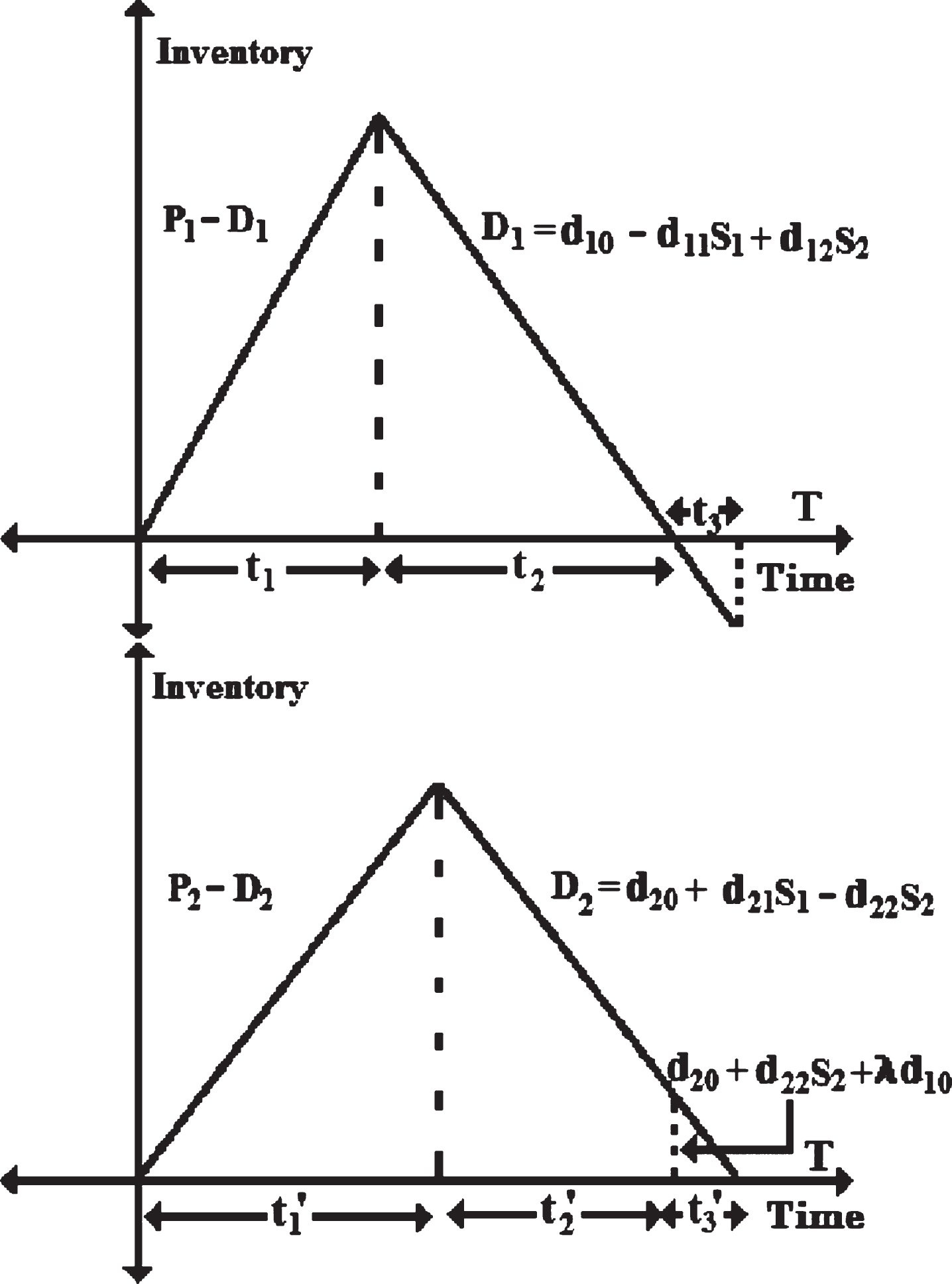
Substitution considering shortage in one of the item with constant demand & same time period.

Fig.3

Nature of 2-D graph considering total profit against selling price (s₁) and (s₂).

Fig.4

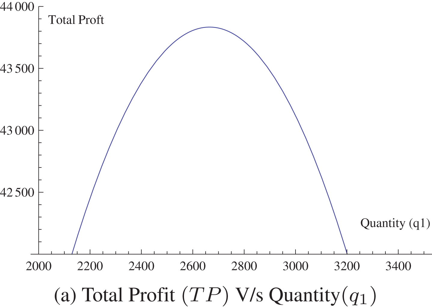
Nature of 2-D graph considering total profit against quantity (q₁).

Fig.5

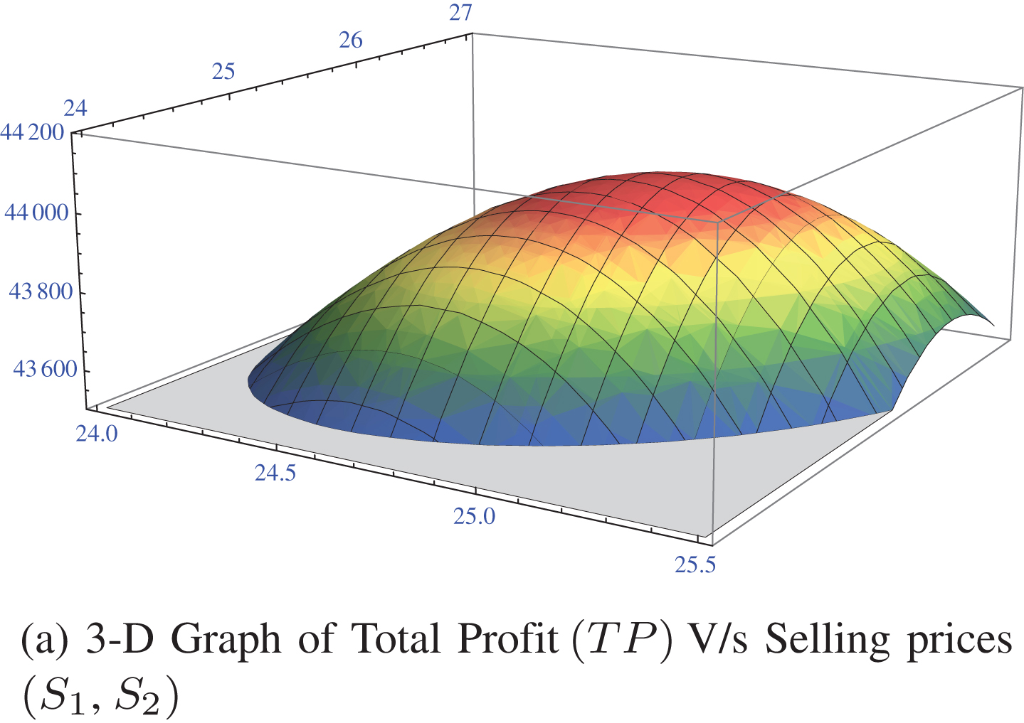
Concavity property of total profit (TP) with respect to selling prices (S₁, S₂) of Model 1.

Fig.6

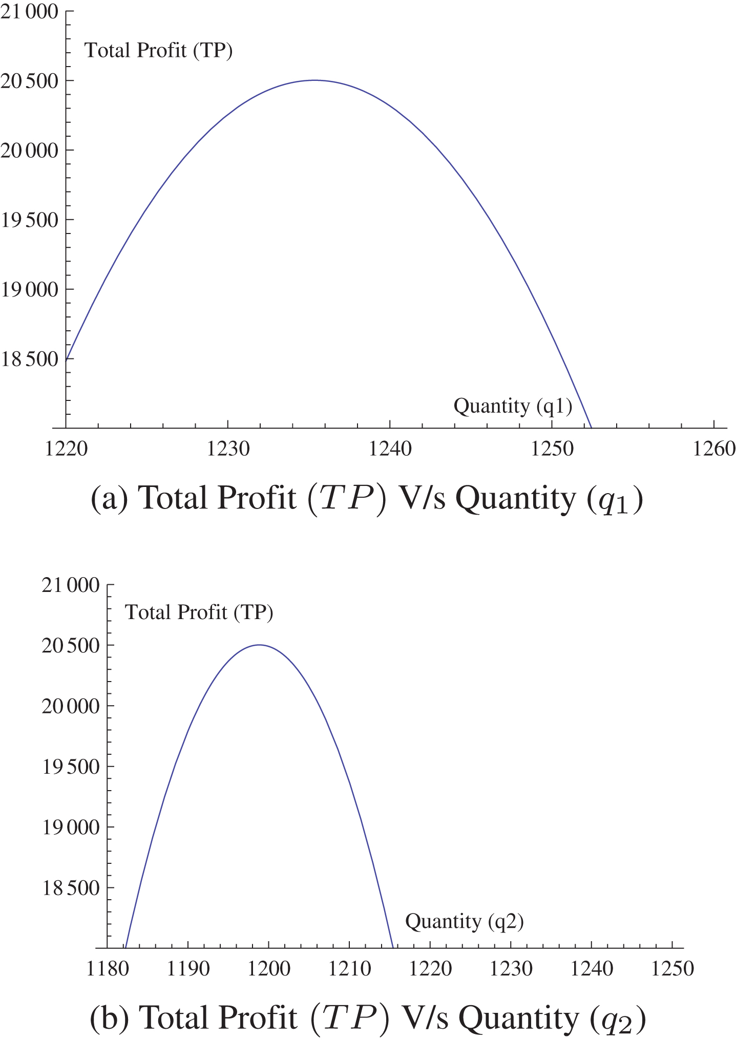
Nature of 2-D graph considering total profit against quantities (q₁) and (q₂).

Fig.7

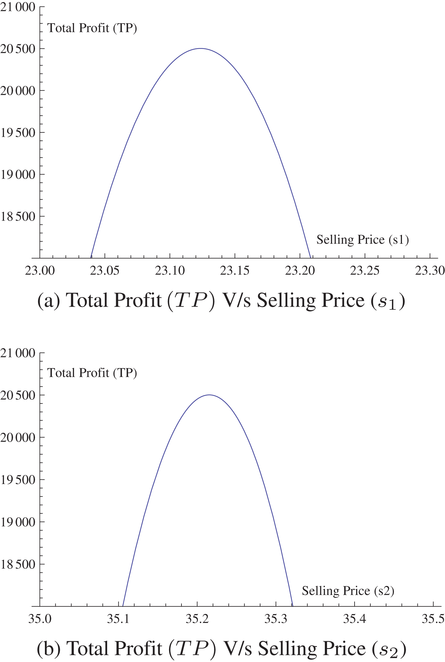
Nature of 2-D graph considering total profit against selling prices (s₁) and (s₂).

Fig.8

Concavity property of total profit (TP) with respect to selling prices (S₁, S₂) of Model 2.

From Figs. 3, 4, 5, 6, 7, 8

Considering the optimal values of Model-1, the Total Profit(TP) is plotted in Figs. 3 and 4 against the different values of s₁, s₂ and q₁ respectively. This shows the nature of the various values corresponding from Table 2 and the peak level on the graph is the maximum value from same table.

Figure 5 is obtained by plotting the Total Profit (TP) against the different values of Selling Prices (s₁ and s₂). This Total profit (TP) maximization is a convex function against selling price rate only.

Considering the optimal values Model-2, the Total Profit (TP) is plotted in Figs. 6 and 7 against the different values of s₁, s₂, q₁ and q₂ respectively. This figure shows the nature of the various values corresponding from Table 3 and the peak level on the graph is the maximum value from same table.

Figure 8 is obtained by plotting the Total Profit (TP) against the different values of Selling Prices (s₁ and s₂). This Total Profit (TP) maximization is a convex function against selling price rate only.

9 Conclusion and future work

In this paper, production cost of the substitutable products on the basis of selling prices and optimum order quantities have been circumscribed over finite time horizon, optimum quantities and production rate cycles so that total profit is maximum. Also, sensitivity analysis have been carried out particularly from the tables based on certain inputs which derives the total profit along with uncertain finite budget constraints. Furthermore, this paper can be extended with others types of production-inventory models such as inventory models with trade credit, two warehouses inventory system, EPQ model with price discount whilst introducing (AUD/IQD) on the substitutable products. Moreover, considering different cases of demand units where one-way substitution i.e. D₂ = 0 or D₁ = 0 individually can also be possible for multi-items also for those products where shortages are entertained from either of the items and vice-versa. This investigation will be helpful for the managers of stores or production cum sale companies where substitutable products are produced and sold.

The virgin ideas presented in this paper are as follows:

Reliability for the production process,

More substitutable products,

Supply-chain system incorporating retailers and customers.

Production cum sale of two substitutable products with can be incurred with effect of selling prices.

References

Bansal

K.K.

and Ahalawat

, Integrated inventory models for decaying items with exponential demand under inflation, International Journal of Soft Computing and Engineering2 (2012), 578–587.

Cárdenas–Barrón

L.E.

, Chung

K.J.

and Treviño–Garza

, Celebrating a century of the economic order quantity model in honor of Ford Whitman Harris, International Journal of Production Economics155 (2014), 1–7.

Cárdenas–Barrón

L.E.

, Treviño–Garza

, Taleizadeh

A.A.

, Treviño–Garza

and Pandian

, Determining replenishment lot size and shipment policy for an EPQ inventory model with delivery and rework, Mathematical Problems in Engineering2015 (2015), 1–8.

Chang

H.C.

, A note on the EPQ model with shortages and variable lead time, Information and Management Sciences15(1) (2004), 61–67.

Charnes

and Cooper

W.W.

, Deterministic equivalents for optimizing and satisficing under chance constraints, Operations Research11 (1963), 18–39.

Chung

K.H.

and Kim

Y.H.

, Economic analysis of inventory systems: A rejoinder, Engineering Economics35 (1989), 75–80.

Dubois

and Prade

, Possibility Theory, New York, London, 1988.

Garg

, Vaish

and Gupta

, An economic production lot size model with price discounting for non-instantaneous deteriorating items with ramp-type production and demand rates, International Journal of Contemporary Mathematical Sciences7(11) (2012), 531–554.

Goyal

S.K.

, A viewpoint on an EOQ model with substitutions between products, Journal of the Operational Research Society46 (1995), 476–477.

10.

Guria

, Das

, mandal

and Maiti

, Inventory policy for an item with inflation induced purchasing price, selling price and demand with immediate part payment, Applied Mathematical Modelling37 (2013), 240–257.

11.

Gurunani

, Economic analysis of inventory systems, International Journal of Production Research21 (1983), 261–277.

12.

Gurunani

and Drezner

, Deterministic hierarchical substitution inventory models, Journal of the Operational Research Society51 (2000), 129–133.

13.

Katagiri

, Sakawa

, Kato

and Nishizaki

, Interactive multi-objective fuzzy random linear programming: Maximization of possibility and probability, European Journal of Operational Research188(2) (2008), 530–539.

14.

Khedlekar

U.K.

, A disruption production model with exponential demand, International Journal of Industrial Engineering Computations3 (2012), 607–616.

15.

Lasdon

L.S.

, Waren

A.D.

, Jain

and Ratner

, Design and testing of a generalised reduced gradient code for nonlinear programming, ACM Transaction on mathematical Software4(1) (1978), 34–50.

16.

Liu

, Theory and Practice of Uncertain Programming, Physica-Verlag, Heidelberg, 2002.

17.

Liu

and Iwamura

K.B.

, Chance constraint Programming with fuzzy parameters, Fuzzy Sets and Systems94 (1998), 227–237.

18.

Maiti

M.K.

and Maiti

, Fuzzy inventory model with two warehouses under possibility constraints, Fuzzy Sets System157 (2006), 52–73.

19.

Merigó

J.M.

, Gil–Lafuente

A.M.

and Yager

R.R.

, An overview of fuzzy research with bibliometric indicators, Applied Soft Computing27 (2015), 420–433.

20.

Merigó

J.M.

, Palacios–Marqués

and Benavides

, Aggregation methods to calculate the average price, Journal of Business Research68 (2015), 1574–1580.

21.

Mishra

S.S.

and Singh

P.K.

, A computational approach to EOQ model with power form stock dependent demand and cubic deterioration, American Journal of Operation Research1 (2011), 5–13.

22.

Moon

and Yun

, An economic order quantity model with a random planning horizon, Engineering Economics39 (1993), 77–86.

23.

Nobil

A.H.

, Sedigh

A.H.A.

and Cárdenas–Barrón

L.E.

, A multi–machine multi–product EPQ problem for an imperfect manufacturing system considering utilization and allocation decisions, Expert Systems with Applications56 (2016), 310–319.

24.

Noori–daryan

A.A.M.

and Cárdenas–Barrón

L.E.

, Joint optimization of price, replenishment frequency, replenishment cycle and production rate in vendor managed inventory system with deteriorating items, International Journal of Production Economics159 (2015), 285–295.

25.

Panda

, Kar

, Maity

and Maiti

, A single period inventory model with imperfect production and stochastic demand under chance and imprecise constraints, European Journal of Operational Research188 (2008), 121–139.

26.

Rao

S.S.

, Engineering Optimization: Theory and Practice, 4th Edition, John Wiley & Sons, Inc., Hoboken, New Jersey, 2009.

27.

Roy

, Maiti

M.K.

, Kar

and Maiti

, An inventory model for a deteriorating item with displayed stock dependent demand under fuzzy inflation and time discounting over a random planning horizon, Applied Mathematical Modelling33 (2009), 744–759.

28.

Seyed

T.A.

, Seyed

H.P.

and Gharaei

, Optimization of a multiproduct economic production quantity problem with stochastic constraints using sequential quadratic programming, Knowledge Based Systems84 (2015), 98–107.

29.

Shamsi

, Haji

, Shadrokh

and Nourbakhsh

, Economic production quantity in reworkable production systems with inspection errors, Scraps and Backlogging, Journal of Industrial and Systems Engineering3 (2009), 170–188.

30.

Singh

and Singh

S.R.

, An EPQ model with power form stock dependent demand under inflationary environment using genetic algorithm, International Journal of Computer Application48(15) (2012), 25–30.

31.

Taleizadeh

A.A.

, Kalantari

S.S.

and Cárdenas–Barrón

L.E.

, Determining optimal price, replenishment lot size and number of shipments for an EPQ model with rework and multiple shipments, Journal of Industrial and Management Optimization11(4) (2015), 1059–1071.

32.

Taleizadeh

A.A.

, Kalantari

S.S.

and Cárdenas–Barrón

L.E.

, Pricing and lot sizing for an EPQ inventory model with rework and multiple shipments, TOP24 (2016), 143–155.

33.

Teng

J.T.

, Ouyang

L.Y.

and Chang

C.T.

, Deterministic economic production quantity model with time-varying demand and cost, Applied Mathematical Modelling29 (2005), 987–1003.

34.

Teng

J.T.

, Ouyang

L.Y.

and Cheng

M.C.

, An EOQ model for deteriorating items with power form stock-dependent demand, Information and Management Science16(1) (2005), 1–16.

35.

Wee

H.M.

, Wang

W.T.

and Yang

P.C.

, A production quantity model for imperfect quality items with shortage and screening constraint, International Journal of Production Research51(6) (2013), 1869–1884.

36.

Widyadana

G.A.

and Wee

H.M.

, Economic Production Quantity (EPQ) deteriorating inventory model with machine breakdown and stochastic repair time, Proceedings of the IEEE International Conference on Industrial Engineering and Engineering Management, Hong Kong, 2009, pp. 548–552.

37.

and Zhou

, Fuzzy Link Multiple-Objective Decision Making, Springer- Verlag, Berlin, 2011.

38.

Zadeh

L.A.

, Fuzzy sets as a basis for a theory of possibility, Fuzzy Sets and Systems1 (1978), 3–28.