Stochastic group shop scheduling with fuzzy due dates

Abstract

The group shop scheduling (GSS) problem is a general formulation that includes the job shop and the open shop scheduling problems. This paper is the first dealing with a GSS problem with random release and processing times and fuzzy due dates. While release and processing times are assumed to be random variables with known distributions, as in many real-world situations, job due dates are considered to be fuzzy tolerating a certain amount of delay. The objective is to maximize the expected total degree of satisfaction with respect to the fuzzy due dates. The problem is formulated as a stochastic disjunctive program and then two solution approaches are developed for it, both of which act within an ant colony optimization (ACO) framework. In the first approach, to estimate the performance of a constructed schedule, each random variable is replaced by its expectation, whereas in the other approach following a simulation optimization procedure, a discrete event simulation model is employed to estimate the performance of a schedule. The proposed approaches are then compared through computational experiments.

Keywords

Group shop scheduling random release times random processing times fuzzy due dates ant colony optimization simulation

1 Introduction

Generally speaking, scheduling is a decision-making process in which limited resources (machines) have to be allocated over time to perform a set of jobs with the objective of optimizing some given criterion. The GSS problem, which frequently occurs in manufacturing environments, is a general form for both the job shop and the open shop scheduling problems, and thus, seems to be a promising research area. In the GSS problem, all operations of a job are partitioned into groups based on their relationship with each other. That is, the operations which are not subject to precedence constraints and can be processed in any order are placed in the same group, while those which have to satisfy precedence constraints are placed in distinct groups. Accordingly, all groups of a job are totally ordered. This NP-hard problem, frequently occurring in industrial environments, was first posed in a mathematical contest in 1997 (http://www.win.tue.nl/whizzkids/1997).

Blum and Samples [5] are among the pioneers that consider the GSS problem. Assuming that all parameters are deterministic, they have developed an ant colony optimization (ACO) algorithm for the problem with the makespan criterion. Liu, et al. [16] have studied the same problem and proposed a tabu search algorithm. Moreover, Ahmadizar and Shahmaleki [10] have considered a similar problem with sequence-dependent setup and transportation times, where jobs are released at different times. They have developed a genetic algorithm (GA) hybridized with an active schedule generator to tackle large-sized problem instances. However, like most other research efforts conducted on scheduling problems, these studies have neglected the uncertainty in parameters. In real-world situations, uncertainty is imposed by the variations in the availability dates, machine breakdowns and so on and hence, considering a scheduling problem with uncertain data is more realistic. Ahmadizar, et al. [8, 9] have considered stochastic group shop scheduling (SGSS) problems subject to random release and processing times. In [8], the total weighted completion time minimization problem has been formulated as a deterministic mixed integer linear programming (MILP) problem, and an ACO algorithm has then been developed for the problem. Moreover, suggesting a lower bound on the expected makespan, Ahmadizar, et al. [9] have developed a simulation-based ACO approach for the makespan minimization problem. Recently, Ahmadizar and Rabanimotlagh [6] have extended the work of Ahmadizar, et al. [9] by taking into consideration an objective function related to job due dates that are known in advance. Furthermore, Ahmadizar and Zarei [7] have considered the GSS problem subject to fuzzy release and processing times. They have prepared the makespan minimization problem in a form of deterministic MILP, and then, developed a GA for the problem.

This study, however, provides an extension to that of Ahmadizar and Rabanimotlagh [6] by taking into consideration the situation with fuzzy job due dates. We consider a SGSS problem where job release times as well as processing times are stochastically distributed, governed by known probability distributions. Ahmadizar and Rabanimotlagh [6] have assumed that the due dates are crisp numbers, whereas in real-world situations, most often a certain amount of delay in due dates is acceptable. Accordingly, in the proposed model, the due dates are considered to be trapezoidal fuzzy numbers, tolerating a certain amount of delay. The objective is to find a job schedule that maximizes the expected total degree of satisfaction with respect to the fuzzy due dates. The problem is formulated as a stochastic disjunctive programming model, and two ACO-based approaches are proposed to tackle it. In the first approach, the performance of a solution to the problem is estimated by replacing all random variables by their expected values, while the other is a simulation optimization procedure in which a discrete event simulation model is employed to estimate the performance of a solution generated in the search process. Both the proposed methods are tested on large instances and comparisons are made. The differences between these two approaches are in their run times and goodness of their results. The first approach can achieve final solutions in less computational times. In contrast, as shown by the computational experiments, the second approach can achieve better results by spending more run times, since it exploits the whole information of the stochastic parameters via simulation optimization procedure. Consequently, the second proposed approach is more suitable to tackle the problem, even though the first one may be appropriate when time is a critical part of the decision making process.

The rest of the paper is organized as follows. In the next section, the problem is introduced and formulated. Section 3 provides an introduction to ACO algorithms and presents the proposed approaches. Section 4 gives computational results, followed by Section 5 concluding the paper.

2 Problem description and formulation

In order to clarify the problem in hand, a short description of the GSS problem is needed. The GSS problem including both the open shop and the job shop scheduling problems is defined as processing a set of jobs on a set of machines. Each job has at most one operation to be processed on each machine. Each job may be processed on at most one machine at a time, and each machine can process at most one job at a time. Preemption is not allowed, that is, each operation must be processed without interruption. All machines are available at time zero. Each job has a release time before which its processing cannot be started. Moreover, setup times are sequence independent, thus included in job processing times, and transportation times are negligible. There exists an unlimited storage capacity between every two machines. In addition, a distinct feature of the GSS problem is that, considering the technological constraints, the operations of each job are partitioned into groups such that the operations in the same group are unordered while those in two distinct groups satisfy the predefined precedence constraint between the groups. If each group consists of only one operation, the GSS problem is equivalent to a job shop scheduling problem. The GSS problem is equivalent to an open shop scheduling problem if all operations of each job belong to just one group. For the sake of simplicity, the following notation is used:

Set of all machines

Set of all jobs

o _ij

Processing of job j on machine i

p _ij

Processing time of operation o_ij

r _j

Release time of job j

{\tilde{d}}_{j}

Due date of job j

C _j

Completion time of job j respect to ${\tilde{d}}_{j}$

μ_j (C_j)

Degree of satisfaction of job j with

An example of the GSS problem consisting of three jobs and three machines is given in Fig. 1(a). Job 1 for example first needs to be processed by machine 1, and next by machines 2 and 3 in any order (i.e., the sequence in which these two processes take place does not matter). So, the operations of job 1 are partitioned into two groups: the first group consists of o₁₁ and the other consists of o₂₁ and o₃₁. A feasible solution to this instance is shown in Fig. 1(b), where the order of processing inside the two groups including more than one operation and the order of processing on the three machines have been determined.

Fig.1

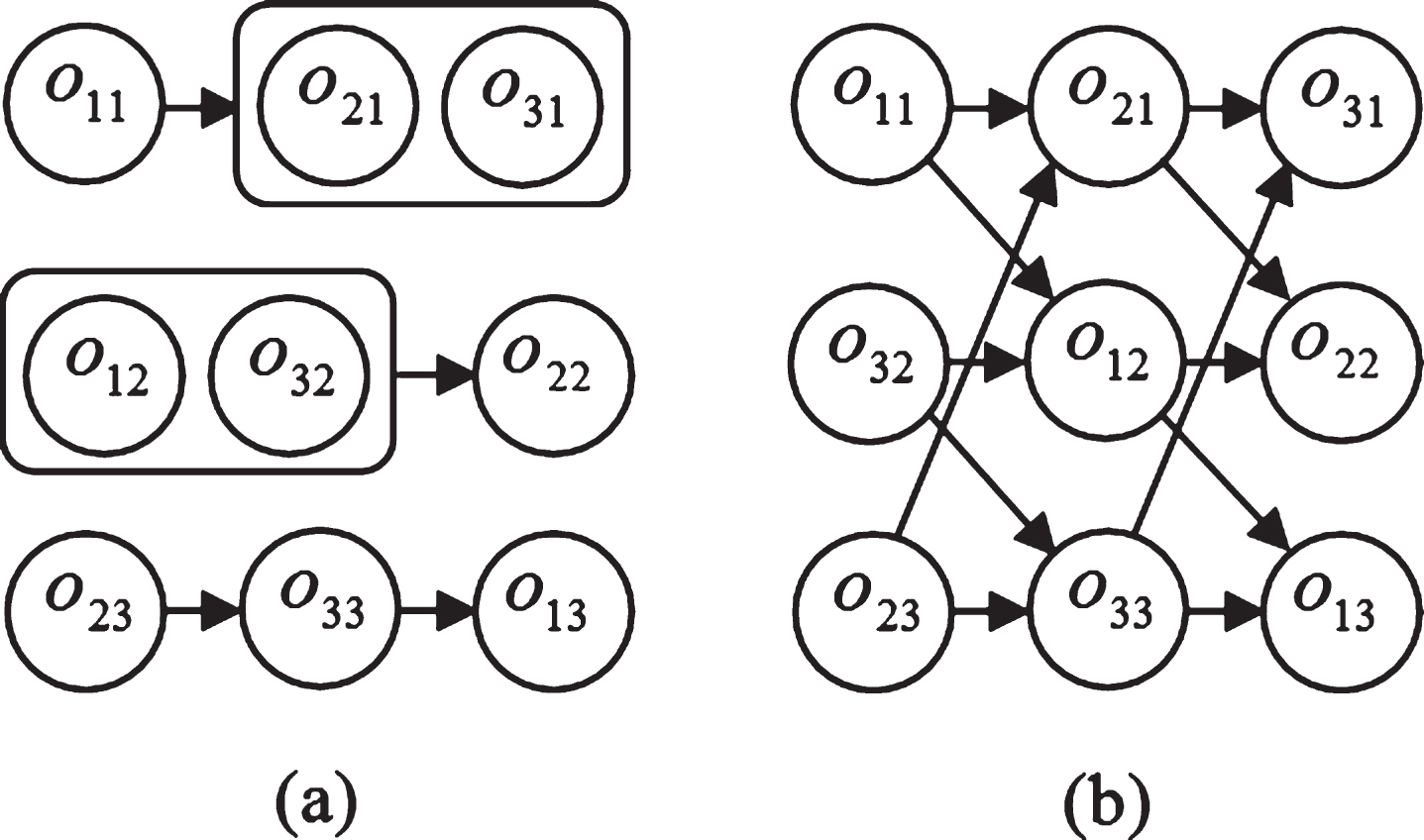
An example of the GSS problem.

In this paper, considering job release and processing times as independent random variables with known probability distributions and job due dates as trapezoidal fuzzy numbers, some potential uncertainties occurring on the shop floor are tackled.

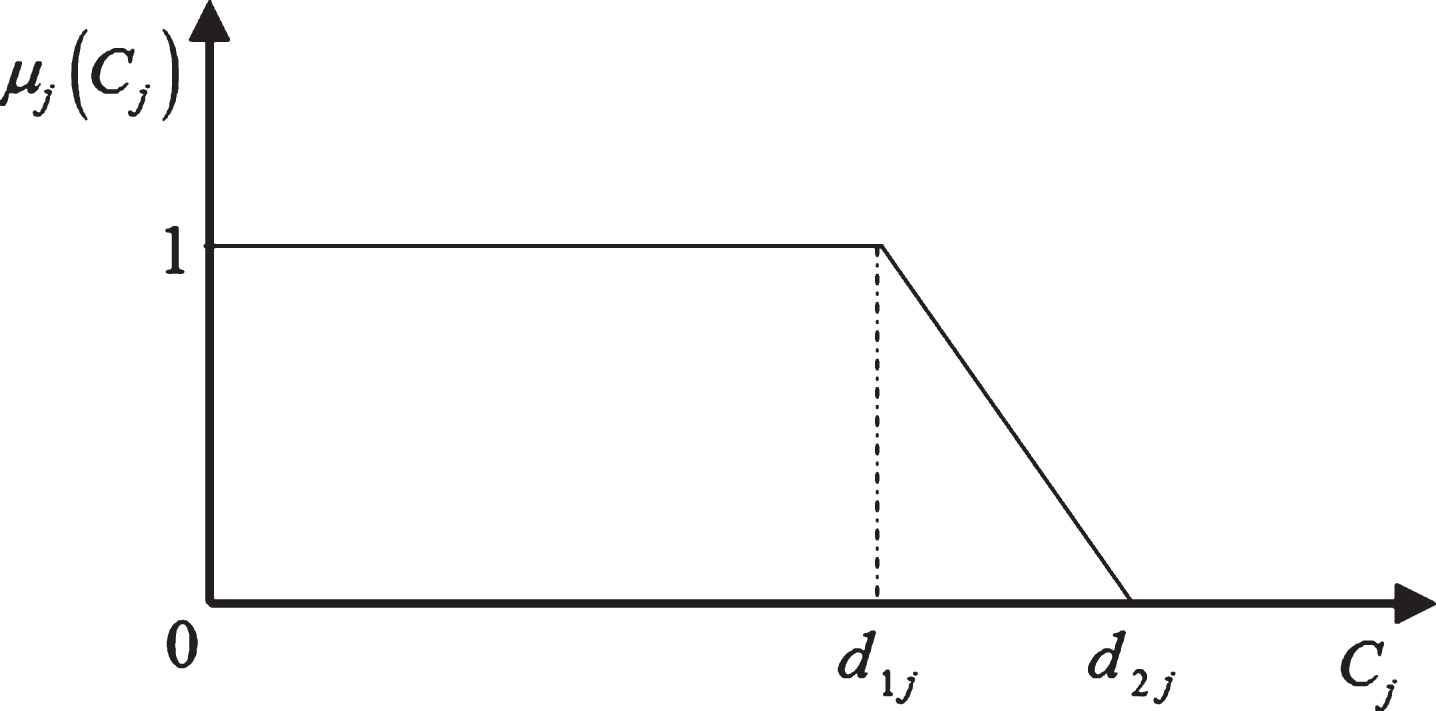
The fuzzy due date of each job j, ${\tilde{d}}_{j}$ , is represented by two real numbers d_1j and d_2j, with d_1j ≤ d_2j. This is due to the fact that most often a certain amount of delay in due date is acceptable. If C_j is not larger than d_1j, the satisfaction degree is 1, i.e., the customer is completely satisfied. If C_j is larger than d_2j, the satisfaction degree is 0. If C_j is larger than d_1j and smaller than d_2j, the satisfaction degree will change between 0 and 1 (see Fig. 2).

Fig.2

Fuzzy due date.

Since the r_j’s and p_ij’s are random variables, C_j’s and thus μ_j (C_j)’s are random variables too. In the problem under consideration, the order of processing inside the groups and the order of processing on the machines have then to be determined in order to maximize the expected total degree of satisfaction with respect to the fuzzy due dates, that is, E [∑_j∈Nμ_j (C_j)].

Lemma 1.If all the due dates are crisp values, the objective function is equivalent to minimizing the expected total number of tardy jobs.

Proof. When d_1j = d_2j for each job j, μ_j (C_j) can take only two values; 0 and 1. Job j with μ_j (C_j) equal to 1 is an on-time job, while job j with μ_j (C_j) equal to 0 is a tardy job. Maximizing E [∑_j∈Nμ_j (C_j)] then becomes maximizing the expected total number of on-time jobs and since the number of jobs is fixed, the proof is completed. ■

Let the decision variable T_ij be the earliest possible starting time of operation o_ij. The problem can then be formulated as the following stochastic disjunctive programming model. $\begin{matrix} min E [\sum_{j} μ_{j} (C_{j})], subject to : \\ T_{ij} \geq r_{j}, \forall o_{ij} \end{matrix}$ (1) $\begin{matrix} T_{ij} - T_{i^{'} j} \geq p_{i^{'} j}, \forall o_{i^{'} j} & o_{ij} with o_{i^{'} j} preceding o_{ij} \end{matrix}$ (2) $\begin{matrix} T_{ij} - T_{i^{'} j} \geq p_{i^{'} j} or T_{i^{'} j} - T_{ij} \geq p_{ij}, \\ \forall o_{i^{'} j} & o_{ij} belonging to the same group \end{matrix}$ (3) $T_{ij} - T_{{ij}^{'}} \geq p_{{ij}^{'}} or T_{{ij}^{'}} - T_{ij} \geq p_{ij}, \forall o_{{ij}^{'}} & o_{ij}$ (4) $C_{j} - T_{ij} \geq p_{ij}, \forall j, o_{ij}$ (5)

Constraints (1) ensure that the processing of each job cannot start before it is released. Constraints (2) ensure that each operation o_ij cannot start before all operations belonging to preceding groups of job j are completed. Disjunctive constraints (3) and (4) ensure that some ordering exists among operations belonging to the same group and among operations requiring the same machine for their execution, respectively. Finally, constraints (5) ensure that the processing of each job cannot complete before all its operations are completed.

To find a feasible solution to the problem, the disjunctive constraints (3) and (4) have to be turned into conjunctive constraints, that is, the order of processing inside the groups and the order of processing on the machines have to be determined, such that the resulting constraints, together with the constraints (1), (2) and (5), are not conflicting.

3 Description of the solution approaches

Nowadays, with the increasing complexity of problems and inability to find the global optimum for large problems in a reasonable amount of time, researchers tend to use metaheuristics which try to find high quality solutions, not necessarily the global optimum, within a reasonable time frame. To approximately solve combinatorial optimization problems, ACO algorithms belonging to the class of constructive metaheuristics simulate the foraging behavior of real ants using simple agents, called artificial ants. The pioneering research effort on ACO has been done by Dorigo [11], and an introduction to the ACO algorithms has then been provided by Dorigo et al. [14]. Performing an incremental construction of solutions by exploiting a probability model indicated by pheromone trails and the heuristic information is the main mechanism underlying ACO. During the search process, to reflect the agents’ acquired search experience, the pheromone trails are updated according to the quality of the solutions constructed, while the heuristic information represents a priori information about the problem or run-time information provided by a source different from the agents. ACO algorithms have so far been successfully applied to a range of optimization problems (see, e.g., [1 , 18]). For more details on ACO, the reader is referred to [13].

In this study, two ACO-based solution approaches are proposed to tackle the problem. The optimization process of these approaches can be expressed as follows (the details are presented later):

Set parameters and initialize the pheromone trails.

While the termination condition is not met, do:

For each ant in the colony, do:

Construct a feasible schedule and apply the pheromone local updating rule;

Evaluate the performance of the generated schedule;

In case of an improved solution, update the best schedule found so far as well as the trail bounds, and then limit the pheromone trails.

Apply the pheromone global updating rule and limit the pheromone trails;

If the restart criterion holds, reset the pheromone trails.

Return the best schedule found.

Although both the developed approaches follow the above algorithm as their optimization process, they are differentiated in the performance evaluation of generated schedules as well as in determining if there is an improvement. In approach 1, while searching the solution space, the performance of a schedule is evaluated by replacing all the random release and processing times by their expectations. Although the idea of replacing each random variable by its expected value seems reasonable when dealing with a stochastic problem, it may not make a good performance analysis. Hence, in approach 2, which is a simulation optimization procedure, the performance of a schedule is evaluated by employing a discrete event simulation model. Since every run of the simulation model (comprised of a total number of 30 replications) provides only an estimation of the objective function value of a solution, the comparison of the solution with the best one found so far is then made through a statistical test at the 0.95 level of confidence. However, in view of the fact that the simulation model is computationally expensive, approach 2 clearly requires more computational time than approach 1.

3.1 Pheromone model

In the proposed approaches, a pheromone model similar to that of Ahmadizar, et al. [8, 9] and Ahmadizar and Rabanimotlagh [6] is employed. To memorize previously generated schedules, pheromone trail $τ_{ij}^{g}$ is associated with the desirability of scheduling operation o_ij in the gth position of its related group and pheromone trail $τ_{ij}^{m}$ with the desirability of scheduling o_ij in the mth position of machine i.

At the initialization step and also each pheromone trails resetting, a fixed value is assigned to all pheromone trails. Then, at run-time they are updated both locally and globally. The pheromone local updating rule has a role in the diversification of the search, while the pheromone global updating rule has a role in the intensification of the search. Moreover, to prevent the approaches from premature convergence to local optima, like the max-min ant system [17], the pheromone trails are always limited between lower and upper bounds.

We calculate a lower bound τ_min and an upper bound τ_max on the pheromone trails as follows: $τ_{max} = \frac{ɛ_{1} Z^{bs}}{ρ n}$ (6) $τ_{min} = ɛ_{2} τ_{max}$ (7) where ɛ₁ is a controlling parameter, ɛ₂ is a parameter between 0 and 1, ρ is the global pheromone evaporating parameter, Z^bs denotes the objective function value of the best schedule found so far, and n is the number of jobs, which is employed tonormalize Z^bs.

Taking the above equations into account, the trail bounds are modified whenever a new best schedule is found; at that time, new upper and lower bounds are calculated and then any pheromone trail out of the range is adjusted (limited), that is, if a pheromone trail is smaller than the new τ_min or greater than the new τ_max, it is set to τ_min or τ_max, respectively. Nevertheless, it is easy to see that when a new best schedule is found, the interval [τ_min, τ_max] shifts to the right, and consequently, this only enforces that those trails having an amount of pheromone smaller than the new τ_min are increased (i.e., the amount of a pheromone trail may not be greater than the new τ_max). Besides, the effect of shifting the interval [τ_min, τ_max] to the right is to allow the pheromone trails related to the new best schedule to be increased to a great extent (i.e., to the new τ_max) by means of the pheromone global updating rule, since, as stated later, this rule is for intensification.

It is noted that, at the starting phase of the proposed approaches, the pheromone trails are set to τ₀, while at the restarting phase the current τ_max is assigned to all of them.

3.2 Schedule construction

In the proposed ACO-based approaches, a list scheduler algorithm [3] is adapted to construct feasible schedules by artificial ants. Starting with a null sequence, an ant builds a permutation of all operations step by step by appending at each step a schedulable operation, whose predecessors all are already scheduled, to the sequence. At each construction step, an operation is chosen from a set of candidates to be sequenced next, i.e., a set of preferred schedulable operations, by applying a probabilistic transition rule. The order of processing inside the groups and the order of processing on the machines, a (feasible) turning of the disjunctive constraints (3) and (4) into conjunctive constraints, are then determined easily according to the generated sequence.

In the following, the notations used in this subsection are listed and then the schedule construction mechanism is presented.

Partial sequence

Set of schedulable operations

Set of exceptional operations

Candidate set

T_{ij}^{PS}

Earliest possible starting time of operation o_ij under PS

C_{ij}^{PS}

Earliest possible completion time of operation o_ij under PS

τ_{ij}^{pos}

heromone trail associated with the desirability of placing operation o_ij in position pos of PS

η_{ij}^{pos}

Heuristic information associated with the desirability of placing operation o_ij in position pos of PS

Begin with PS as the null partial sequence. Initially, SO includes all operations belonging to the first group of every job.

For pos = 1 to total number of operations, do the following:

Identify the exceptional operations and include them in EO;

If EO is not null, select an operation from EO at random. Otherwise, identify the subset CS of SO, and then, select an operation from CS by means of the transition rule;

Put the selected operation in position pos of PS;

Remove the operation from SO, and if it is the last operation sequenced among the operations belonging to the same group, add all operations belonging to the direct successor group, if it exists, to SO.

According to the generated sequence, determine the order of processing inside the groups and the order of processing on the machines.

3.2.1 Exceptional operations

We refer to a schedulable operation o_ij as an exceptional operation if it is the only remaining unscheduled operation requiring machine i and also the only remaining unscheduled one belonging to its related group. Clearly, if such an operation o_ij is added to the partial schedule as soon as possible, the operations belonging to the next group of job j, if it exists, are included in the set of schedulable operations sooner, and this may lead to a better schedule.

3.2.2 Candidate list strategy

To guide the search towards promising regions of the solution space, at each construction step, a set (or list) of candidate operations, i.e., a subset of schedulable operations preferred to be sequenced next, is determined. Let π^PS denote the earliest completion time among all operations in SO under PS, that is, $π^{PS} = min_{o_{ij} \in SO} C_{ij}^{PS}$ . According to the candidate list strategy, CS consists of all operations o_ij in SO for which $T_{ij}^{PS} < π^{PS}$ . However, since $T_{ij}^{PS}$ and $C_{ij}^{PS}$ (and thus π^PS) are random variables, in both of the proposed approaches they are estimated by replacing all of the random release and processing times by their expected values. Denote the resulting values by ${\hat{T}}_{ij}^{PS}$ and ${\hat{C}}_{ij}^{PS}$ , respectively; obviously, ${\hat{C}}_{ij}^{PS} = {\hat{T}}_{ij}^{PS} + E (p_{ij})$ . As a result, π^PS can be estimated by $min_{o_{ij} \in SO} {\hat{C}}_{ij}^{PS}$ . It is noted that the rule ${\hat{T}}_{ij}^{PS} < π^{PS}$ has been used since the experimentation with different rules, including those that result in active and non-delay schedules [15], has shown it to perform the best.

3.2.3 Transition rule

Let q₀ be a parameter determining the relative importance of exploitation versus exploration. An artificial ant chooses one of the operations from CS to be placed in position pos of PS according to a transition rule so-called pseudo-random proportional rule [12] as follows. With probability q₀, the ant selects the operation o_ij for which the product between the pheromone trail and the heuristic information is maximum (exploitation), that is, $o_{ij} = argmax ({(τ_{ij}^{pos})}^{α} {(η_{ij}^{pos})}^{β})$ , where α and β are two parameters determining the relative importance of the pheromone trail and the heuristic information. While with probability 1 - q₀, the ant selects an operation o_ij according to the following probability distribution (exploration): $Pr (o_{ij}) = \frac{{(τ_{ij}^{pos})}^{α} {(η_{ij}^{pos})}^{β}}{\sum_{o_{i^{'} j^{'}} \in CS} {(τ_{i^{'} j^{'}}^{pos})}^{α} {(η_{i^{'} j^{'}}^{pos})}^{β}}, \forall o_{ij} \in CS$ (8)

The pheromone trail $τ_{ij}^{pos}$ is determined by $\min (τ_{ij}^{g}, τ_{ij}^{m})$ if placing operation o_ij in position pos of PS results in placing it in the gth position of its related group and in the mth position of machine i. Nevertheless, if o_ij is the last operation that is sequenced among the operations belonging to the same group, $τ_{ij}^{pos}$ is determined only by $τ_{ij}^{m}$ ; and if o_ij is the last operation that is sequenced among the operations requiring machine i, $τ_{ij}^{pos}$ is determined only by $τ_{ij}^{g}$ . It is noted that if o_ij is the last operation that is sequenced among the operations belonging to the same group and also among those requiring machine i, it is selected as an exceptional operation.

Moreover, the heuristic information $η_{ij}^{pos}$ is calculated according to the earliest due date and the earliest starting time first rules as follows: $η_{ij}^{pos} = \frac{1}{d_{j}} \times \frac{1}{1 + {\hat{T}}_{ij}^{Ps}}, \forall o_{ij} \in CS$ (9) where d_j denotes the defuzzified due date of job j, i.e., a realization of ${\tilde{d}}_{j}$ . To defuzzify ${\tilde{d}}_{j}$ , which is a right trapezoidal fuzzy number, a number y in the interval (0, 1) is considered; d_j is then the point such that its degree of membership is equal to y, that is, μ_j (d_j) = y. We choose y to be 0.9. Clearly, d_j is a number in the interval (d_1j, d_2j).

3.3 Pheromone updating rules

While constructing a schedule, to decrease its desirability and thus to explore different areas of the solution space by the next ants in the colony, the local updating rule is applied to each pheromone trail $τ_{ij}^{g}$ and $τ_{ij}^{m}$ corresponding to the schedule. Suppose that operation o_ij has been placed in position pos of PS, resulting in placing it in the gth position of its related group and in the mth position of machine i. Depending on which pheromone trails have been used in the $τ_{ij}^{pos}$ determination, both or one (or even none, in the case of an exceptional operation) of the following pheromone updates are then applied:

$\begin{matrix} τ_{ij}^{g} & = & (1 - ρ^{'}) τ_{ij}^{g} + ρ^{'} τ_{min} \\ τ_{ij}^{m} & = & (1 - ρ^{'}) τ_{ij}^{m} + ρ^{'} τ_{min} \end{matrix}$ (10) where ρ′ is the local pheromone evaporating parameter.

Moreover, once all ants in the colony have constructed their schedules, the pheromone trails are globally updated. Each pheromone trail is first evaporated, that is,

$\begin{matrix} τ_{ij}^{g} & = & (1 - ρ) τ_{ij}^{g} \\ τ_{ij}^{m} & = & (1 - ρ) τ_{ij}^{m} \end{matrix}$ (11)

However, this may cause the amount of a pheromone trail to be smaller than τ_min, and consequently, such pheromone trails are set to τ_min. Then, to make the search more directed, an extra amount of pheromone is deposited on each pheromone trail $τ_{ij}^{g}$ and $τ_{ij}^{m}$ corresponding to the best schedule found so far as follows (again, for some operations only one or even none of the two updates may be essential):

$\begin{matrix} τ_{ij}^{g} & = & τ_{ij}^{g} + ρ \frac{ɛ_{1} Z^{bs}}{n} \\ τ_{ij}^{m} & = & τ_{ij}^{m} + ρ \frac{ɛ_{1} Z^{bs}}{n} \end{matrix}$ (12)

From Equations (6, 11 and 12), and that ρ is a parameter smaller than 1, it is then easy to show that the global updating rule may not cause the amount of a pheromone trail to be greater than τ_max.

4 Computational results

To assess the performance of the developed approaches, the only real GSS instance, called whizzkids97 (http://www.win.tue.nl/whizzkids/1997), is used. It is a large enough instance that consists of 15 machines, 20 jobs, and 197 operations partitioned into 124 groups. Since in the original instance all jobs are available at time zero, the job release times are defined the same as in [8, 9]. Moreover, the (crisp) job due dates are defined the same as in [6].

In order to transform this GSS instance to various instances of the problem under consideration, the release and processing times are assumed to be normal, uniform or exponential random variables and the due dates to be right trapezoidal fuzzy numbers. The mean of the random variables as well as the d_1j values are then set to be equal to the corresponding values in the GSS instance. The standard deviation for each normal or uniform variable is given as the ratio to its mean, referred to as the variability. Moreover, the d_2j value for each job j is given as the ratio to its d_1j, referred to as the fuzziness. For simplicity, without loss of generality, the distribution and variability for all the random variables as well as the fuzziness for all the due dates are assumed to be the same. Several values for the variability, 0.05, 0.1, 0.15, 0.2, 0.25, 0.3 and 1, as well as for the fuzziness, 1.05, 1.1, 1.15 and 1.2, are then considered, thus providing a total of 60 problem instances. It is noted that the variability for an exponential random variable is equal to 1 due to the fact that its mean and standard deviation are equal.

The approaches have been coded in C# and run on a 3.60 GHz Pentium IV PC with 1 GB memory. To set up the algorithm parameters, an approach similar to that of Yagmahan and Yenisey [4] has been employed. Initially, all parameters have been set each as a fixed value. These fixed values, due to the similarity of the problem basics, have been determined as those used in [6]. In each step, one of the parameters has then been tested through repeating each test for five times; after which, five candidate values have been obtained for each parameter. Testing all combinations of candidate values for the parameters on the instances, the following has been obtained as the most appropriate setting for the parameters: τ₀ = 0.01, ɛ₁ = 0.05, ɛ₂ = 0.01, ρ = 0.05, ρ′ = 0.01, q₀ = 0.95, α= 1 and β= 0.3. There are five ants in the colony and each approach terminates when the total number of iterations reaches 14000. In addition, if the best found solution does not improve within 400 successive iterations, the pheromone trails are reset. For the second approach, the number of replications to simulate each generated solution is set as 30, on the basis of preliminary experiments; in such a case, the simulation model performs reasonably in terms of both run-time and the performance estimation quality.

For each of the proposed approaches, each problem instance has been tested for five trials, and the best solution achieved among the five trials has been chosen as the final output. Then, to have a fair and good comparison, the performance of each of the final schedules has been measured by utilizing a discrete event simulation model, where the number of simulation runs is set to be 10000. The computational results are shown in Tables 1–3, which give for each instance the estimated objective function values of the solutions achieved by both of the approaches.

Table 1
Computational results under normally distributed release and processing times

Fuzziness

1.05 1.10 1.15 1.20

Variability Approach 1 Approach 2 Approach 1 Approach 2 Approach 1 Approach 2 Approach 1 Approach 2

0.05 14.27 14.06 14.29 14.39 14.92 14.86 15.37 15.71

0.10 12.84 13.17 13.61 13.66 14.14 14.25 14.80 14.88

0.15 11.30 12.13 11.40 12.57 12.35 13.38 13.80 13.97

0.20 8.81 11.10 10.34 11.45 12.42 12.44 12.83 13.16

0.25 9.11 10.51 11.87 10.65 11.14 11.99 11.52 11.78

0.30 7.36 9.22 8.84 9.77 9.36 11.03 10.37 11.11

1.00 3.05 4.41 3.27 4.70 3.55 4.82 4.26 5.21

	Fuzziness
0.05	14.27	14.06	14.29	14.39	14.92	14.86	15.37	15.71
0.10	12.84	13.17	13.61	13.66	14.14	14.25	14.80	14.88
0.15	11.30	12.13	11.40	12.57	12.35	13.38	13.80	13.97
0.20	8.81	11.10	10.34	11.45	12.42	12.44	12.83	13.16
0.25	9.11	10.51	11.87	10.65	11.14	11.99	11.52	11.78
0.30	7.36	9.22	8.84	9.77	9.36	11.03	10.37	11.11
1.00	3.05	4.41	3.27	4.70	3.55	4.82	4.26	5.21

Table 2

Computational results under uniformly distributed release and processing times

	Fuzziness
	1.05		1.10		1.15		1.20
Variability	Approach 1	Approach 2	Approach 1	Approach 2	Approach 1	Approach 2	Approach 1	Approach 2
0.05	13.80	14.72	15.04	14.29	15.35	15.05	15.31	15.58
0.10	13.19	13.39	14.17	14.06	14.68	14.56	14.40	15.19
0.15	12.91	12.00	12.20	13.54	13.53	14.13	14.32	14.84
0.20	10.12	11.78	11.26	12.32	12.58	13.07	12.16	13.78
0.25	8.49	11.07	9.95	11.39	11.62	12.02	12.47	13.01
0.30	8.05	10.33	10.58	10.94	9.72	11.80	11.21	12.30
1.00	3.41	4.33	3.61	4.24	3.97	4.45	3.94	4.94

Table 3

Computational results under exponentially distributed release and processing times

	Fuzziness
	1.05		1.10		1.15		1.20
Variability	Approach 1	Approach 2	Approach 1	Approach 2	Approach 1	Approach 2	Approach 1	Approach 2
1.00	3.25	4.23	3.32	4.72	3.73	5.39	4.69	5.41

As anticipated, the results presented in Tables 1–3 confirm that, under identical conditions, as the variability of the release and processing times grows, the objective function value decreases, while as the fuzziness of the due dates grows, the objective function value increases (the exceptions in the tables are due to the stochastic nature of the proposed ACO-based approaches). Nevertheless, the distribution type of the random variables has no significant impact on the value of the objective function. The reason is that in most real-world situations, as in the problem instances, ∑_j∈Nμ_j (C_j) which is a random variable is composed of a large number of independent random variables, and consequently, from the central limit theorem it follows an approximately normal distribution. With this in mind, the results for the instances where the release and processing times follow normal or uniform distributions with the variability of 1 are compatible with those shown in Table 3.

The comparison of the solutions achieved by the two approaches for each problem instance is then made through a statistical test at the 0.95 level of confidence. Tables 4–6 provide the comparison results with number 0 indicating no significant difference in the performance of the proposed approaches, number 1 indicating the better performance of approach 1 and number 2 indicating the better performance of approach 2. At the 0.95 level of confidence, among the 60 instances, approach 2 has shown a better performance in 51 cases which means that it is more appropriate to tackle the problem. However, approach 1 requires remarkably less computational effort; each run of approach 1 takes on average 110 seconds, while each run of approach 2 takes on average 255 seconds. It should also be noted here that the distribution type of the random variables has no effect on the CPU time of approach 1, while that of approach 2 is affected since the time to generate a random number in the simulation phase varies depending on the distribution type. Hence, approach 1 may be more appropriate to tackle the problem in the situations where time is a very important issue.

Table 4

Comparison results under normally distributed release and processing times

	Fuzziness
Variability	1.05	1.10	1.15	1.20
0.05	1	2	1	2
0.10	2	2	2	2
0.15	2	2	2	2
0.20	2	2	0	2
0.25	2	1	2	2
0.30	2	2	2	2
1.00	2	2	2	2

Table 5

Comparison results under uniformly distributed release and processing times

	Fuzziness
Variability	1.05	1.10	1.15	1.20
0.05	2	1	1	2
0.10	2	1	1	2
0.15	1	2	2	2
0.20	2	2	2	2
0.25	2	2	2	2
0.30	2	2	2	2
1.00	2	2	2	2

Table 6

Comparison results under exponentially distributed release and processing times

	Fuzziness
Variability	1.05	1.10	1.15	1.20
1.00	2	2	2	2

5 Conclusions

In this paper, a GSS problem with uncertain data has been considered. The GSS problem provides a general formulation including two other shop scheduling problems, the job shop and the open shop.

Job release times as well as processing times are stochastically distributed with known distributions, while job due dates are represented by trapezoidal fuzzy numbers. The objective is to find a job schedule maximizing the expected total degree of satisfaction with respect to the fuzzy due dates. When all the due dates are crisp values, the objective function considered is equivalent to minimizing the expected total number of tardy jobs. After formulating the problem as a stochastic disjunctive program, two ACO-based solution approaches have been proposed and then compared through computational experiments. In the proposed approaches, an algorithm is employed to construct a feasible schedule in which schedulable operations are added to the schedule one after another. However, the two approaches differ in the way in which the objective function value of a constructed solution is estimated. In the first approach, the performance of a schedule is measured by replacing all random variables by their expectations, while in the other which is a simulation optimization procedure it is measured in a more realistic way by employing a discrete event simulation model. The first approach can achieve final solutions in less computational times as compared to the second approach. On the other hand, since the second approach exploits the whole information of the stochastic parameters via simulation optimization procedure, it can achieve better results by spending more run times. Therefore, in the situations where time is a very important issue, the first approach seems to be more effective in finding relatively good solutions in short computational times. In contrast, the second approach is more suitable in the situations where time is less important.

References

Biniaz

and Abbasi

, Unsupervised ACO: Applying FCM as a supervisor for ACO in medical image segmentation, Journal of Intelligent & Fuzzy Systems27 (2014), 407–417.

Khanra

, Maiti

M.K.

and Maiti

, A hybrid heuristic algorithm for single and multi-objective imprecise traveling salesman problems,in press, Journal of Intelligent & Fuzzy Systems. doi: 10.3233/IFS-151913

Giffler

and Thompson

G.L.

, Algorithms for solving production scheduling problems, Operations Research8 (1960), 487–503.

Yagmahan

and Yenisey

M.M.

, Ant colony optimization for multi-objective flowshop scheduling problem, Computers & Industrial Engineering54 (2008), 411–420.

Blum

and Samples

, An ant colony optimization algorithm for shop scheduling problems, Journal of Mathematical Modelling and Algorithms3 (2004), 285–308.

Ahmadizar

and Rabanimotlagh

, Group shop scheduling with uncertain data and a general cost objective, International Journal of Advanced Manufacturing Technology70 (2014), 1313–1322.

Ahmadizar

and Zarei

, Minimizing makespan in a group shop with fuzzy release dates and processing times, International Journal of Advanced Manufacturing Technology66 (2013), 2063–2074.

Ahmadizar

, Ghazanfari

and Fatemi Ghomi

S.M.T.

, Application of chance-constrained programming for stochastic group shop scheduling problem, International Journal of Advanced Manufacturing Technology42 (2009), 321–334.

Ahmadizar

, Ghazanfari

and Fatemi Ghomi

S.M.T.

, Group shops scheduling with makespan criterion subject to random release dates and processing times, Computers & Operations Research37 (2010), 152–162.

10.

Ahmadizar

and Shahmaleki

, Group-shop scheduling with sequence-dependent set-up and transportation times, Applied Mathematical Modelling38 (2014), 5080–5091.

11.

Dorigo

, Optimization, learning and natural algorithm (in Italian), Ph. D. Thesis, Politecnico di Milano, 1992.

12.

Dorigo

and Gambardella

L.M.

, Ant colony system: A cooperative learning approach to the traveling salesman problem, IEEE Transactions on Evolutionary Computingl (1997), 53–66.

13.

Dorigo

and Stutzle

, Ant Colony Optimization, MIT Press, Cambridge, 2004.

14.

Dorigo

, Maniezzo

and Colorni

, The ant system: Optimization by a colony of cooperating agents, IEEE Transactions on Systems, Man, and Cybernetics Part B26 (1996), 29–41.

15.

Pinedo

, Scheduling: Theory, Algorithms and Systems (4rd Ed.), Springer, 2012.

16.

Liu

S.Q.

, Ong

H.L.

and Ng

K.M.

, A fast tabu search algorithm for the group shop scheduling problem, Advances in Engineering Software36 (2005), 533–539.

17.

Stutzle

and Hoos

H.H.

, The MAX-MIN Ant System and local search for the traveling salesman problem, The Proceedings of the IEEE International Conference on Evolutionary Computation, New York, 1997, pp. 308–313.

18.

Sun

and Ma

, The power distribution network structure optimization based on improved ant colony algorithm, Journal of Intelligent & Fuzzy Systems26 (2014), 2799–2804.