Time series forecasting using fuzzy transformation and neural network with back propagation learning

Abstract

In this study, a hybrid time series approach has been proposed in which the fuzzy transform (F-transform) is employed for its ability of handling uncertainty due to noise and multilayer perceptron with back propagation learning for its good adapting capability. F-transform is used to decompose the time series data and then those decomposed data are used as inputs and original data are used as targets in the neural networks with back propagation (BPNN) learning to capture the pattern of original time series. Proposed approach is used in Composite Index of Shanghai Stock Exchange data collected for the period January, 1993 to December, 2009. The result is compared with the result obtained by using de-noising capability of wavelet transform along with back propagation neural network. This study also includes an empirical analysis for the forecasting of Bombay Stock Exchange SENSEX data collected for the period January, 2002 to August, 2014 and Australian electricity market – Price.

Keywords

Fuzzy transform neural network with back propagation learning time series prediction stock market data

1 Introduction

Recent trends of time series forecasting are based on the methods of data analysis as neural networks, fuzzy sets, rough sets etc. There are some time series observations like university enrollments, financial and medical time series which are short, imprecise and non-regular in nature. Such type of time series observations can not be analyzed by commonly used statistical methods. A considerable part of the real time series with imprecise observations can be handled by fuzzy techniques. F-transform is one of the important tools which is used for data decomposition specially for short time series.

Perfilieva [1] introduced fuzzy transform (F-transform) to bridge among other kinds of transform from classical methods, namely, Fourier transform, Laplace transform, wavelet transform and fuzzy approximation techniques. Hossein et al. [2] proposed a hybrid model based on local linear neuro fuzzy and fuzzy transform for prediction of energy consumption. It is shown that their model integrated with F-transform has been improved the forecasting accuracy. Novák et al. [3] proposed a new methodology for the analysis and forecasting of time series by hybridizing two techniques: F-transform and the perception-based logical deduction. They concluded that the F-transform and the fuzzy/linguistic rules are useful to compute long term forecasts without the influence of any kind of error correction and learning from the experience type model of forecasting. Perfilieva et al. [4] developed the two-term additive decomposition time series model, where first term is used for capturing the low-frequency trend by F-transform and second term is used for residual vector, which is treated as a stationary time series based on fuzzy tendency modeling.

Preprocessing of the time series by extracting important features or sometimes de-noising are useful to analyze the nature of it. Chaplot et al. [5] developed a time series model where features were extracted based on discrete wavelet transform and used as inputs in neural network self-organizing maps and support vector machine for classification of magnetic resonance (MR) images of the human brain. Huang et al. [6] proposed Empirical Mode Decomposition (EMD), a data analysis method for nonlinear and non-stationary time series by decomposing a time series into a small number of independent and implicational intrinsic modes based on scale separation. Zhang et al. [7] proposed Ensemble EMD (EEMD), an improvement of EMD which can better separate the scales naturally by adding white noise series to the original time series and then treating the ensemble averages as the true intrinsic modes. Muhammad et al. [8] proposed a hybrid wavelet based artificial neural network and concluded that the pre-processing of input rainfall data by wavelet transform increased the performance of the neural network models. They have shown a comparative study on Haar wavelet, Daubechies Wavelet (db), Coiflets (Coif), Symlets (Sym) and Meyer wavelet (mey). Matsumoto and Watada [9] proposed a method to model the chaotic portion from the data of small-dimensional space and increased the forecasting precision. Some economic data are not sufficiently chaotic to apply chaos theory, so it is difficult to analyze those time series data and capture the future trend. Time series data are first decomposed in small parts by wavelet transform and chaotic nature of every part has been analyzed. They observed that highly chaotic part helped in forecasting near future with 70% accuracy on the up-and-down movement of the TOPICS value.

Wang et al. [10] developed an algorithm of wavelet de-noising-based back propagation neural network for stock price time series prediction. They used Daubechies wavelet(db3) and compared their work with the simple neural network with back propagation learning. Wang and Gupta [11] also used wavelet analysis to de-noise the data and predicted future stock prices using neural network.

Zhang and Qi [12] studied the effectiveness of data preprocessing, including deseasonalization and detrending, on neural network modeling and forecasting performance. They concluded that neural networks were not able to capture seasonality or trend variations effectively with the unpreprocessed raw data and either detrending or deseasonalization can dramatically reduce forecasting errors. Moreover, a combined detrending and deseasonalization was found to be the most effective data preprocessing approach.

In this paper, F-transform and neural network with back propagation learning have been used for stock exchange time series prediction as well as Australian electricity market – Price.

The remainder of this paper is organized as follows. Section 2 presents the basic concepts of F-transform and neural network with back propagation learning. The model which combines the F-transform and neural network with back propagation (BPNN) learning is described in Section 3. In Section 4, there is numerical illustration. In Section 5, the computational results have been analyzed. Finally, the conclusions and future research directions are presented in Section 6.

2 Basic concepts

F-transform and multilayer perceptron with back propagation learning are discussed in this section.

2.1 Fuzzy transform

For any transformation the basic idea is to transform an original space into a special space of functions for analyzing and mining information. Then transform back to the original space either to reveal the original data or some near estimation of original data [1]. Similar ideas are followed in case of F-transform also. It can be applied to a continuous function defined on a fixed interval, say [a, b] ⊂ R (set of real numbers). The F-transform maps the original space into a space consists of a finite vector of numbers on the basis of basic functions of fuzzy partitions of the given domain or universe. Inverse transform maps the transformed values into a function which is near approximation of the original function.

Definition: Let x₁ < x₂ < . . . < x_n be fixed nodes in [a, b], such that x₁ = a, . . . , x_n = b and Fuzzy sets A₁, A₂, . . . , A_n have their membership functions A₁ (x) , A₂ (x) , . . . , A_n (x) defined on [a, b], form a fuzzy partition if they satisfy the following conditions for k = 1, 2, . . . , n: $\begin{matrix} 1 . A_{k} : [a, b] \to [0, 1], A_{k} (x_{k}) = 1, \\ 2 . A_{k} (x) = 0 if x \notin (x_{k - 1}, x_{k + 1}) where \\ x_{1} = a and x_{n} = b, \\ 3 . A_{k} (x) is continuous, \\ 4 . A_{k} (x), k = 2, 3, . . ., n are strictly increasing \\ on [x_{k - 1}, x_{k}] and A_{k} (x), k = 1, 2, . . ., n - 1 \\ are strictly decreasing on [x_{k}, x_{k + 1}], \\ 5 . For all x \in [a, b] \sum_{k = 1}^{n} A_{k} (x) = 1 \end{matrix}$ (1) $\begin{matrix} 6 . A_{k} (x_{k} - x) = A_{k} (x_{k} + x), for all x \in [0, h], \\ k = 2, . . ., n - 1 where all x_{1}, x_{2}, . . ., x_{n} s \\ are equidistant, i . e ., x_{k} = a + h (k - 1), \\ k = 1, . . ., n, h = \frac{b - a}{n - 1} \\ 7 . A_{k} (x) = A_{k - 1} (x - h), for all k = 2, . . ., n - 1 \\ and x \in [x_{k}, x_{k + 1}], and \\ A_{k + 1} (x) = A_{k} (x - h), for all k = 2, . . ., n - 1 \\ and x \in [x_{k}, x_{k + 1}] where h = \frac{b - a}{n - 1} . \end{matrix}$ where h is a length of the support of A₁ and A_n, 2h is the support of other basic functions A_k, k = 2, 3, . . . , n - 1 in case of uniform partition. The membership functions A₁, A₂, . . . , A_n are called basic functions.

F-transform: Let C ([a, b]) be the set of continuous functions on the domain [a, b], A₁, A₂, . . . , A_n are basic functions on [a, b] and let f be any function in C ([a, b]). Then n-tuple vector of real numbers [F₁, F₂, . . . , F_n] is defined by $F_{k} = \frac{\int_{a}^{b} f (x) A_{k} (x) dx}{\int_{a}^{b} A_{k} (x) dx}, k = 1, 2, . . ., n .$ (2) is called the F-transform of f with respect to A₁, A₂, . . . , A_n.

In case of discrete F-transform, f be given at nodes p₁, p₂, . . . , p_l and A₁, A₂, . . . , A_n, n < l are basic functions which form a fuzzy partition on [a, b], then [F₁, F₂, . . . , F_n] are given by $F_{k} = \frac{\sum_{j = 1}^{l} f (p_{j}) A_{k} (p_{j})}{\sum_{j = 1}^{l} A_{k} (p_{j})}$ (3) F-transform of f is denoted by F_n [f].

Components from continuous as well as discreteF-transform of a function are the weighted mean values of that function where the weights are obtained by the basic functions [1].

Inverse F-transform: The function is reconstructed by inverse F-transform which are near approximation of the original function or sometime it can be the original one.

Let A₁, A₂, . . . , A_n be basic functions forming a fuzzy partition on [a, b], f be a function from set of continuous functions C ([a, b]) and F_n [f] = [F₁, F₂, . . . , F_n] be n-tuple vector which basically denotes F-transform of f with respect to the basic functions, then the inverse F-transform f_F,n can be defined as $f_{F, n} = \sum_{k = 1}^{n} F_{k} A_{k} (x)$ (4)

Theorem [1]:Let f be a continuous function on [a, b], then for any ɛ > 0 there exist n_ɛ and a fuzzy partition A₁, A₂, . . . , A_{n
_ɛ}of [a, b] such that for all x ∈ [a, b] $| f (x) - f_{F, n_{ɛ}} (x) | \leq ɛ,$ (5)where f_{F,n_ɛ} is the inverse F-transform of f with respect to the fuzzy partition A₁, A₂, . . . , A_{n
_ɛ}.

This theorem states that after applying inverse F-transform on some function which is transformed by F-transform, we get near approximation of the original function.

Example: Let us considering a function, f (p) = p², where f (0) =0, f (0.5) =0.25, f (1) =1, f (1.5) =2.25, f (2) =4, f (2.5) =6.25, f (3) =9 and partitioning the interval (0, 3) with h = 0.6 i.e., x = [0 0.6 1.2 1.8 2.4 3]. We are finding the basic functions using triangular membership functions which is given below: $\begin{matrix} A_{1} (p) = {\begin{matrix} 1 - \frac{(p - x_{1})}{h_{1}}, & p \in [x_{1}, x_{2}] \\ 0, & otherwise \end{matrix} \\ A_{k} (p) = {\begin{matrix} \frac{(p - x_{k - 1})}{h_{k - 1}}, & p \in [x_{k - 1}, x_{k}] \\ 1 - \frac{(p - x_{k})}{h_{k}}, & p \in [x_{k}, x_{k + 1}] \\ 0, & otherwise \end{matrix} \end{matrix}$ (6) $A_{n} (p) = {\begin{matrix} \frac{(p - x_{n - 1})}{h_{n - 1}}, & p \in [x_{n - 1}, x_{n}] \\ 0, & otherwise \end{matrix}$ where h₁ = x₂ - x₁, h_k-1 = x_k - x_k-1, h_k = x_k+1 - x_k, h_n-1 = x_n - x_n-1. We are using Equation (3) to get the transformed value of f (x) at k = 1, 2, 3, 4, 5, 6. Basic functions can be written in matrix form whose elements are a_kj, k = 1, 2, 3, 4, 5, 6 and j = 1, 2, 3, 4, 5, 6, 7. The basic functions are given in Table 1.

Table 1

Values of basic functions in matrix form

	p ₁	p ₂	p ₃	p ₄	p ₅	p ₆	p ₇
A ₁	1	1/6	0	0	0	0	0
A ₂	0	5/6	1/3	0	0	0	0
A ₃	0	0	2/3	1/2	0	0	0
A ₄	0	0	0	1/2	2/3	0	0
A ₅	0	0	0	0	1/3	5/6	0
A ₆	0	0	0	0	0	1/6	1

Using Equation (3), we get F₁ = f (p₁) +1/6 * f (p₂), F₂ = 5/6 * f (p₂) +1/3 * f (p₃), F₃ = 2/3 * f (p₃) +1/2 * f (p₄), F₄ = 1/2 * f (p₄) +2/3 * f (p₅), F₅ = 1/3 * f (p₅) +5/6 * f (p₆) and F₆ = 1/6 * f (p₆) + f (p₇).

Using equation Equation (4), we get the inverse F-transform values which are f_F,6 (p₁) = F₁, f_F,6 (p₂) =1/6 * F₁ + 5/6 * F₂, f_F,6 (p₃) =1/3 * F₂ + 2/3 * F₃, f_F,6 (p₄) =1/2 * F₃ + 1/2 * F₄, f_F,6 (p₅) =2/3 * F₄ + 1/3 * F₅, f_F,6 (p₆) =5/6 * F₅ + 1/6 * F₆ and f_F,6 (p₇) = F₆.

2.2 Neural network with back propagation learning

In this paper, neural network with three layers naming input, hidden and output have been used with back propagation learning. Basic steps of the algorithm are given below.

Step 1: Weight initialize with uniformly distributed random numbers in (0, 1) in between layers.

Step 2: Perform Steps 3-9 when stopping condition is false.

Step 3: Perform Steps 4-8 for each training pair.

Feed forward phase:

Step 4: Calculate the values in hidden layer using Equation (7). $z_{inj} = v_{0} + Σ_{i = 1}^{n} x_{i} v_{ij}, j = 1, 2, . . ., p$ (7) where x_i, i = 1, 2, . . . , n are inputs and p denotes number of nodes in hidden layer. Calculate the output of hidden unit by applying activation function over z_inj using Equation (8) $z_{j} = f (z_{inj})$ (8) and send it in to the nodes of output layer.

Step 5: Calculate the values in output layer using Equation (9) $y_{ink} = w_{0} + Σ_{j = 1}^{p} z_{j} w_{jk}, k = 1, 2, . . ., m$ (9) and apply the activation function to compute the output signal using Equation (10) $y_{k} = f (y_{ink}) .$ (10)

Back propagation of error:

Step 6: Calculate error terms for all output units. For a unit, say k, of the output layer, the calculated error or change of weight, denoted by δ_k and defined by $δ_{k} = (t_{k} - y_{k}) f^{'} (y_{ink})$ (11) where t_ks are targets and y_ks are outputs.

Calculate change of weight Δw_jk using error correction term δ_k and learning rate α as below $Δ w_{jk} = α δ_{k} Z_{j} .$ (12)

Also, send δ_k to the hidden layer backwards.

Step 7: For a unit, say j, of the hidden layer, the calculated error or change of weight, denoted by δ_inj as $δ_{inj} = Σ_{k = 1}^{m} δ_{k} w_{jk} .$ (13)

The term δ_inj gets multiplied with the derivative of f (z_inj) to calculate the error term: $δ_{j} = f^{'} (z_{inj}) δ_{inj} .$ (14)

Calculate change of weight Δv_ij using error correction term δj and learning rate α as below $Δ v_{ij} = α δ_{j} x_{i} .$ (15)

Weight updates:

Step 8: Each output unit y_k, k = 12, . . . , m updates the weights: $w_{jk} (new) = w_{jk} (old) + Δ w_{jk} .$ (16)

Each hidden unit z_j, j = 1, . . . , p updates the weights: $v_{ij} (new) = v_{ij} (old) + Δ v_{ij} .$ (17)

Step 9: Check for the stopping condition. The stopping condition is certain number of epochs reached.

3 Learning algorithm for F-transform based BPNN

In this section, we present a learning scheme for proposed model. Figure 1 illustrates the flowchart of the learning algorithm for F-transform based BPNN model. In the proposed model, data is decomposed first using fuzzy transformation [1]. Total data set is broken into blocks of four data points. Each data points of the time series are equally time spaced points. To utilize fuzzy transformation, we interpolate one new point within first and second time series data point and another within second and third time series data point of each block, in this way we get seven fixed points of each block. We are using Equation (3) to get F-transform of each block, where f (x_i) , i = 1, 2, 3, . . .s are time series data points, A_k (x)s are basic functions at k = 1, 2, . . . , n. 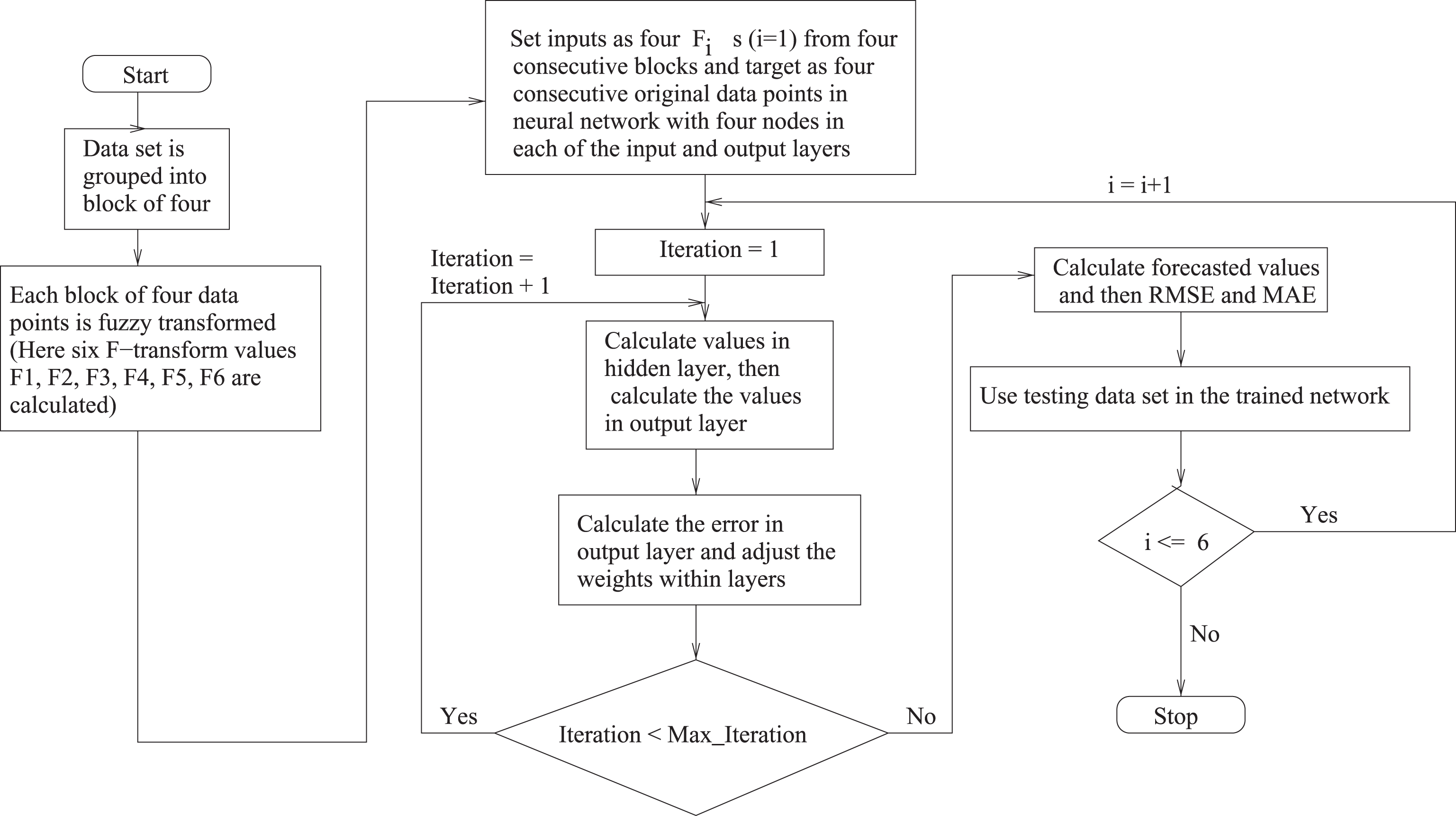Those $F_{k}^{'}$ s from consecutive blocks are used as inputs in the input layer of the neural network, where as target values are time series data points. In this way, training is completed. Test data sets are used to feed forward to the neural network with adjusted weights.

Fig.1

Flowchart of the learning algorithm for F-transform based BPNN.

From the error measurement and the test data set, we have tried to find which F_ks are able to approximate the original time series mostly. We concluded from that the set of those $F_{k}^{'}$ s are good to handle uncertainty due to noise of the noisy time series.

Steps of the proposed algorithm are as follows.

Step 1: Data points are broken into blocks of four data points.

Step 2: Fuzzy transforms F₁, F₂, . . . , F_n for each block have been calculated.

Step 3: Six neural network models F1NN, F2NN, F3NN, F4NN, F5NN and F6NN are constructed where F_k, (k = 1, 2, . . . , n)s are inputs of F_kNN, (k = 1, 2, . . . , n) respectively and original data points are targets.

After completion of training, testing data sets are used to test the proposed model.

4 Numerical illustration

Proposed model is applied on some data sets namely Shanghai Stock Exchange, Bombay Stock Exchange data and Australian electricity market – Price.

We have compared our work with the work by Wang et al. [10]. They have developed the wavelet de-noising-based back propagation neural network and used discrete wavelet transform with Daubechies wavelet on 204 trading months of SCI closing price collected on the Shanghai Stock Exchange from January 1993 to December, 2009. They have trained their model with 80% training data set and the remaining worked as testing data set. We have been able to collect the same data from January, 1993 to December, 2009, total 204 trading months. In our case, 70% of the collected data are used as training data set and remaining is used for testing purpose.

Also we have considered the data set on Bombay Stock Exchange SENSEX closing price collected from January, 2002 to August, 2014 [13] for further analysis. We have used 152 data points in the proposed model, of which 70% is used for training purpose and the remaining is used for testing purpose.

Another time series on Australian electricity price [14, 15] from September, 2013 to September, 2014 is collected as real life time series to observe the performance of the proposed model. Here, the results from the work by Gromov and Borisenko [14] is compared with our proposed idea using this time series. Also, data of four weeks in the year 2004 are collected to compare with other models mentioned in [14].

5 Result of the proposed algorithm

Forecasting is an important field of learning or adopting as it helps human being to take right decision at right moment. In case of stock market data, the movement of itself is uncertain due to several factors and hence it is noisy. So, it is really hard to decide for stock investors about their buying and selling of stocks. Predictions will be accurate when the historical data are de-noised as sudden ups and downs are removed. Wavelet transform is utilized to de-noise data and then fit those in neural network models. In our work, we have used fuzzy transform to serve the same purpose and then fit those de-noised data in neural network with back propagation learning to predict the movement of stocks from those data.

Number of basic functions is user defined, hence the number of FkNN will be same as number of basic functions. Proposed models are always compared with existing models to show the improvement and a comparison is perfect only when the methods are formed by considering same environment. We have compared our work with work in [10], where six models are developed. So, we have modeled our concepts in such a way that it is also developing six models i.e., k = 6 is considered here.

In the proposed model, we have calculated sixF-transform, say, F₁, F₂, . . . , F₆ for each block of four data points with six basic functions and seven fixed nodes of equal length. We have formed six neural network models with back propagation learning where inputs are F₁s for F1NN, F₂s for F2NN,..., F₆s for F6NN respectively.

Each model has four nodes in input layer, four nodes in hidden layer and four nodes in output layer in case of Shanghai Stock Exchange data. Similar architecture for BPNN is used in case of Bombay Stock Exchange data. Figure 2 depicts the diagram of the six models FkNN, k = 1, 2, . . . , 6 for Shanghai Stock Exchange Data.

Fig.2

Diagram of the six models FkNN, k = 1, 2, . . . , 6 for Shanghai Stock Exchange Data.

The RMSE and MAE values of both SSE CI and BSE closing price data for each six models are shown in Tables 2 and 3 respectively.

Table 2

Calculated prediction error for SSE CI closing price data

Models		RMSE		MAE
Proposed	Wang	Proposed	Wang	Proposed	Wang
approach	et al.	approach	et al.	approach	et al.
	[10]		[10]		[10]
F1NN	BP1	47.445681	2006.2	32.529069	1620.6
F2NN	BP2	47.519164	1412.7	32.621868	1038.4
F3NN	BP3	48.318567	1984.4	33.464119	1340.3
F4NN	BP4	49.702843	847.5841	34.087774	675.9543
F5NN	BP5	52.236336	1349.7	34.991938	1067.1
F6NN	BP6	55.163081	1619.1	37.012279	1377.7

Table 3

Calculated prediction error for BSE closing price data

Models	RMSE	MAE
F1NN	131.750792	78.787953
F2NN	131.592500	78.381104
F3NN	132.014587	77.641627
F4NN	132.607425	76.796036
F5NN	133.403105	76.262693
F6NN	135.213216	78.608221

Figures 5 and 6 depict the respective original data for SSE CI and BSE and their inverse F-transform data. Figure 3 depicts the original data and all the test results for F₁, F₂, F₃, F₄, F₅ and F₆ for SSE CI data. Training and test results for individual F₁, F₂, F₃, F₄, F₅ and F₆ of SSE CI data are shown in Fig. 7(a), 7(b), 7(c), 7(d), 7(e) and 7(f) respectively. Figure 4 depicts the original data and all the test results for F₁, F₂, F₃, F₄, F₅ and F₆ for BSE data. Training and test results for individual F₁, F₂, F₃, F₄, F₅ and F₆ of BSE data are shown in Fig. 8(a), 8(b), 8(c), 8(d), 8(e) and 8(f) respectively.

Fig.3

Original SSE CI data and corresponding forecasted results.

Fig.4

Original BSE Sensex data and corresponding forecasted results.

Fig.5

Original SSE CI data and corresponding inverseF-transform data.

Fig.6

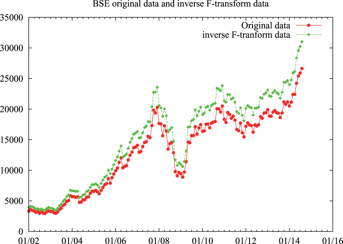
Original BSE data and corresponding inverse F-transform data.

Fig.7

Original Shanghai data and corresponding forecasted results.

Fig.8

Original BSE data and corresponding forecasted results.

In Table 2, calculated RMSE and MAE for the proposed model and model by Wang et al. [10] are compared. It is observed that our models are capable for forecasting with less prediction error. Results of testing data set by our model are shown in Figs. 3 and 4 for the two time series. The models which have bold face values are best model for our case and for the work by Wang et al. [10] respectively in Table 2.

In Table 3, model which have bold face value is best for BSE data set in our work.

Tables 4 and 5 show the results on Australian electricity market – Price. Table 4 shows the RMSE, MAE and MER with respect to different number of nodes in input and output layer of our approach. It shows that MER are lesser in comparison to the work in [14] than RMSE and MAE. Table 5 shows the better performance of proposed approach comparison to DWT, MLP, SVM, PSF and PCW where the time series on Australian electricity market – Price has been considered of four weeks from different months of the year 2004.

Table 4

RMSE, MAE and MER of the time series Australian electricity market – Price with different numbers of nodes in input and output layer

RMSE	MAE	MER(%)	Number of nodes
16.295491	8.958653	0.1572	4 input, 4 output
16.243604	9.521210	0.1671	5 input, 5 output
13.581258	4.394545	0.0771	10 input, 10 output

Table 5

MER for some weeks of the year 2004 (Australian electricity market – Price) [14]

Week	DWT	MLP	SVM	PSF	PCW	Proposed
	(%)	(%)	(%)	(%)	(%)	approach (%)
Second of January	12.94	25.81	23.37	15.62	1.33	0.15
First of July	12.23	8.36	15.03	9.12	1.47	0.11
First of August	16.17	15.85	36.18	13.98	1.28	0.07
Third of December	10.01	47.41	33.74	10.23	1.11	0.09
Average	12.84	24.36	27.08	12.23	1.30	0.105

DWT: Discrete wavelet transform, MLP: Multilayer perceptron, SVM: Support vector machine, PSF: Pattern sequence-based forecasting, PCW: predictive clustering with Wishart clustering algorithm.

6 Conclusion

In this paper, we proposed a hybrid algorithm to predict the time series of the Shanghai (composite index), Bombay (SENSEX) stock exchange and Australian electricity market – Price, where good results are obtained and shows that this algorithm is efficient in respect to forecasting errors compare to others.

Simulation results show that proposed algorithm with F-transform based preprocessing of data outperforms the algorithms where wavelet transform based preprocessing of data has been used along with BPNN in both data processing transformation.

In addition, the proposed hybrid learning algorithm has been used to get more than six F-transform value as it will approximate the curve with more accuracy. We have used triangular membership functions to compute basic functions of F-transform, so other membership functions can be tested to get the basic functions, also higher order fuzzy logic can be implemented.

Footnotes

Acknowledgments

The first author would like to thank DST INSPIRE, India for their help and supports to sustain the work.

Appendix

References

Perfilieva

, Fuzzy transforms: Theory and applications, Fuzzy Sets and Systems157 (2006), 993–1023.

Iranmanesh

, Abdollahzade

and Miranian

, Forecasting energy consumption using fuzzy transform and local linear neuro fuzzy models, International Journal on Soft Computing (IJSC)2(4) (2011), 11–24.

Novák

, Štěpnička

, Dvořák

, Perfilieva

, Pavliska

and Vavříčková

, Analysis of seasonal time series using fuzzy approach, International Journal of General Systems39(3) (2010), 305–328.

Perfilieva

, Yarushkina

, Afanasieva

and Romanov

, Time series analysis using soft computing methods, International Journal of General Systems42(6) (2013), 687–705.

Chaplot

, Patnaik

L.M.

and Jagannathan

N.R.

, Classification of magnetic resonance brain images using wavelets as input to support vector machine and neural network, Biomedical Signal Processing and Control1 (2006), 86–92.

Huang

N.E.

, Shen

and Long

S.R.

, The empirical mode decomposition and the Hilbert for nonlinear and nonstationary time series analysis, Process of the Royal Society of LondonA 454 (1998), 903–995spectrum.

Zhang

, Lai

K.K.

and Wang

S.Y.

, A new approach for crude oil price analysis based on Empirical Mode Decomposition, Energy Economics30 (2008), 905–918.

Shoaib

, Shamseldin

A.Y.

and Melville

B.W.

, Comparative study of different wavelet based neural network models for rainfall-runoff modeling, Journal of Hydrology515 (2014), 47–58.

Matsumoto

and Watada

, A wavelet transform approach to chaotic short-term forecasting, Time Series Analysis, Model, & Applications47 (2013), 177–197.

10.

Wang

J.Z.

, Wang

J.J.

, Zhang

Z.G.

and Guo

S.P.

, Forecasting stock indices with back propagation neural network, Expert Systems and Applications38 (2011), 14346–14355.

11.

Wang

and Gupta

, Neural networks and wavelet denoising for stock trading and prediction, Time Series Analysis, Model, & Applications47 (2013), 229–247.

12.

Zhang

G.P.

and Qi

, Neural network forecasting for seasonal and trend time series, European Journal of Operational Research160 (2005), 501–514.

13.

Bombay stock exchange SENSEX data collected from the website “”, –http://www.bseindia.com/indices/indexarchivedata.aspx.

14.

Gromov

V.A.

and Borisenko

E.A.

, Predictive clustering on non-successive observations for multi-step ahead chaotic time series prediction, Neural Computing & Application26 (2015), 1827–1838.

15.

Martinez-Alvarez

, Troncoso

, Riquelme

J.C.

and Aguilar-Ruiz

J.S.

, Energy time series forecasting based on pattern sequence similarity, IEEE Transactions on Knowledge and Data Engineering23(8) (2011), 1230–1243.