A fuzzy-wavelet denoising technique with applications to noise reduction in audio signals

Abstract

In most of the data analysis tools, the sensitivity toward noise exists. Since real data is always contaminated by noise, a preprocessing technique to reduce noise is of interest. We propose a new method to eliminate noise using the fuzzy wavelet technique. We decompose a function using fuzzy wavelets to extract detail and approximation coefficients. Consequently, we threshold the detail coefficients to reduce the effect of noise and reconstruct a denoised signal. This new method exhibits robust behavior even applied for signals with a very small signal to noise ratio. It shows better results compared to ordinary wavelet denoising and fuzzy denoising on very irregular data. We apply the proposed method to noise reduction in audio signals and compare it with ordinary wavelet denoising. The obtained results are satisfactory.

Keywords

Fuzzy transform wavelet transform thresholding wavelet denoising

1 Introduction

On one hand, real-world data is always corrupted by noise. Since most of the data analysis tools are sensitive to noise, it is very important to perform a preprocessing to reduce noise before using these tools. On the other hand, wavelet denoising techniques are popular techniques for signal extraction and denoising (see for instance, [4 , 17, 20]).

Consider the following noisy model: $Y_{i} = f (x_{i}) + ɛ_{i}, i = 1, . . ., n and x_{i} \in τ,$ (1) where ɛ = (ɛ₁, ɛ₂, …, ɛ_n) ′ ∼ N (0, σ²I) is the noise with unknown σ², I is an identity matrix with size n and f (x_i) is a function to be estimated defined on some index set $τ \subset ℝ$ , without any parametric assumptions such as linearity. Inference about f such as its estimation is of interest. We construct an estimator based on fuzzy wavelet transform using one of the three fuzzy transforms given in [11].

Singular Spectral Analysis (SSA) can be considered as an effective nonparametric tool to denoise noisy signals [19] but it is only efficient for very smooth models with a high signal to noise ratio.

Several types of transformations such as Fourier, Laplace and wavelet are used as effective tools to construct an approximation of a model. The core idea of these tools consists in transforming an original function space into a space with simpler computations. The inverse transform produces either the original function (perfect reconstruction) or its approximation.

Using ordinary wavelet transform, we estimate f or denoise Y with the following steps:

Step 1: Decompose (Y₁, …, Y_n) by wavelet transform to obtain wavelet coefficients up to level J;

Step 2: Threshold wavelet coefficients based on a thresholding strategy;

Step 3: Apply inverse wavelet transform on the thresholded detail coefficients and the approximation coefficients to obtain a denoised version of Y.

Hereafter, wavelet denoising method is denoted by (WD). For more details about this method see [3 , 20].

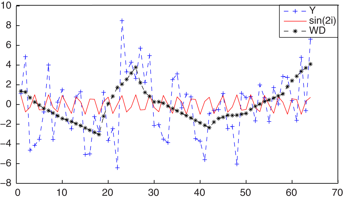
As we can see in these papers, this method works well in most cases. Nevertheless, for small signal to noise ratio (SNR) or for an irregular function of interest, WD method does not give satisfactory result. To illustrate this fact, see the following example. Consider the model Y_i = sin(2i) + ɛ_i where $ɛ_{i} \overset{iid}{\sim} N (0, 8)$ ; i = 1, …, 64 with small SNR. In Fig. 1, data and WD fit are denoted by squo+’ and squo*’ respectively and sin(2i) is plotted in the solid curve. Figure 1 shows that the estimate obtained by WD is not similar to sin(2i) which shows it is not a good estimation of this function. In this example, we use hard threshold and Daubechies wavelet with 2 vanishing moments. This wavelet family has been commonly used in different applications of wavelets, see for example [16].

Fig.1

Wavelet denoising of Y_i = sin(2i) + ɛ_i (shown by ‘+’), sin(2i) (solid curve) and WD (shown by ‘*’).

Since the noise level is high, WD method cannot approximate f well. Hence for some functions and models, we need to use a method to denoise with more precision.

Perfilieva [11] developed three techniques for fuzzy transform (or, shortly, F-transform). The main idea of F-transform is a fuzzy partition of the domain into fuzzy subsets. A simple approximation of the original function is accessible via the inverse formula of the F-transform.

Perfilieva and Hodakova [10] proved that the inverse F-transform has efficient filtering properties. Beg and Aamir [8] developed the notion of fuzzy wavelets and proved a theorem establishing properties of fuzzy wavelets using filtering properties of F-transform. They have extended fuzzy multiresolution analysis schemes to the fuzzy wavelets.

The structure of the paper is as follows. In Section 2, the concept of fuzzy partition, F-transform, inverse F-transform and fuzzy wavelet transform are introduced. In Section 3, fuzzy wavelet denoising is proposed. Section 4 contains some simulation examples to compare fuzzy wavelet denoising, ordinary wavelet denoising and fuzzy denoising. The proposed method is applied to audio signals in Section 5. The paper is concluded in Section 6.

2 Preliminaries

The F-transform is a transformation that can be applied to a continuous function with a bounded domain or discrete function with a finite domain. The domain of function is partitioned to fuzzy sets. The F-transform takes a function and transfers it to a real vector, i.e. it produces a set-to-point correspondence between the partitions and the average values of the function. Let [a, b] be the space of points, a fuzzy set 𝒜 in [a, b] is characterized by a membership function A (x) which associates each point in [a, b] to a real number in the interval [0, 1]. The value of A (x) represents the “grade of membership” of x in 𝒜.

Suppose the domain of a function is the interval [a, b]. In what follows, the fuzzy partition is given by fuzzy subsets of this interval.

Let x₁ < … < x_n be fixed real numbers in the interval [a,b] such that x₀ = a, x_n+1 = b and n ≥ 2. Let 𝒜₁, …, 𝒜_n be the fuzzy sets characterized with their membership functions A₁ (x) , …, A_n (x). They constitute a fuzzy partition of [a,b], if they satisfy the following conditions for k = 1, …, n:

A_k : [a, b] → [0, 1] , A_k (x_k) =1;

A_k (x) =0 if x ∉ (x_k-1, x_k+1);

A_k (x) is continuous;

A_k (x) is strictly increasing on [x_k-1, x_k] for k = 2, …, n, and A_k (x) is strictly decreasing on [x_k, x_k+1] for k = 1, …, n - 1;

∀ x ∈ [a, b], $\sum_{k = 1}^{n} A_{k} (x) = 1$ .

The membership functions A₁ (x) , …, A_n (x) are called basic functions. If the points x₁, …, x_n are equidistant then the fuzzy partition 𝒜₁, …, 𝒜_n, n > 2, is uniform, i.e. x_k = a + (k - 1) h, k = 1, …, n, where $h = \frac{(b - a)}{(n - 1)}$ . Furthermore, two following properties are fulfilled for k = 2, …, n - 1:

A_k (x_k - x) = A_k (x_k + x), for all x ∈ [0, h];

A_k (x) = A_k-1 (x - h), for all x ∈ [x_k, x_k+1] and A_k+1 (x) = A_k (x - h), for all x ∈ [x_k, x_k+1].

Let f be any continuous function in [a, b] and S_△x,n = {A_1,△x, …, A_n,△x} be a set of basic functions which form a fuzzy partition of [a, b] where △x is the support of each basic function. We say that the n-tuple of real numbers [ℱ₁, …, ℱ_n] given by: $ℱ_{k} = \frac{\int_{a}^{b} f (x) A_{k} (x) dx}{\int_{a}^{b} A_{k} (x) dx} k = 1, \dots, n$ (2) is the (integral) F-transform of f with respect to A₁, …, A_n.

The inverse F-transform of a function f (with respect to A₁, …, A_n) is a linear combination of the F-transform components ℱ_n [f] = [ℱ₁, …, ℱ_n] and A₁, …, A_n. Then the function: $f_{ℱ, n} (x) = \sum_{k = 1}^{n} ℱ_{k} A_{k} (x)$ (3) is called the inverse F-transform of f with respect to A₁, …, A_n.

We can reconstruct the function from its F-transform components by inverse F-transform but we lose some information because this is not a perfect reconstruction [11].

For a function f given at points p₁, p₂, …, p_l ∈ [a, b], we define its discrete F-transform by n-tuple of real numbers [F₁, …, F_n] if we use a summation instead of the integral in Equation (2). Therefore, the discrete F-transform of the function f is given as follows with respect to basic function A₁, …, A_n, n ≤ l: $F_{k} = \frac{\sum_{i = 1}^{l} f (p_{i}) A_{k} (p_{i})}{\sum_{i = 1}^{l} A_{k} (p_{i})}; k = 1, \dots, n .$ (4)

In the case of discrete F-transform, we define the inverse F-transform only at points where the original function is given: $f_{F, n} (p_{j}) = \sum_{k = 1}^{n} F_{k} A_{k} (p_{j})$ (5) see [5, 11] for more details. Hereafter, for simplicity, we use the expression F-transform instead of the expression discrete F-transform.

Let A (x) be a fuzzy basic function but centered at the first point, i.e., k = 0; such that, A_k (x) = A (x - x_k) = A (x_k - x). The shift operator R_k is defined as follows: $R_{k} A (x) = A_{k} (x) .$ (6)

The components of F_n [f] are weighted mean values of f where the weights are given by the basic functions. For each value of p_i in (x_i-1, x_i+1), we have a different approximation of the original function [11].

We consider p_i = i for i = 1, …, l and we normalize the values of A by dividing them by $\sum_{i = 1}^{l} A_{k} (p_{i})$ . For the sake of simplicity, hereafter, we use the notation A for normalized one. Then without loss of generality, we assume that l = n and we can express Equation (4) as follows [10]: $F_{k} = \sum_{i = 1}^{n} A (k - i) f (i); k = 1, \dots, n .$ (7)

In this case, F_k is a convolution of two functions f and A i.e., F_k = A ∗ f.

If A (x) be a fuzzy basic function, its reflection, $\tilde{A}$ , is defined as follows: $\tilde{A} (x) = A (- x)$ (8) for x ∈ [a, b]. In the discrete case, we have: $\tilde{A} (i) = A (- i) = A (n - i)$ (9) for all i ≤ n and $n \in ℕ$ .

Let $M \in ℕ$ and n = 2M. A set of fuzzy orthonormal basis is of the form ${R_{2 k} A}_{k = 1}^{M} \cup {R_{2 k} AT}_{k = 1}^{M}$ , which is called the first stage fuzzy wavelets and A is the generator of the first stage fuzzy wavelet basis, where $AT (i) = (- 1)^{i} A (n - i) = (- 1)^{i} \tilde{A} (i)$ for i = 1, …, n, [8].

For fuzzy wavelet transform orthonormality holds in the fuzzy sense i.e., basic functions are approximately orthonormal. As a result, there was not a perfect reconstruction with an approximation of the original function.

To obtain next stages of decomposing Y, we consider n as the maximum number of fuzzy basic functions to approximate f (x) such that it is divisible by 2^p, where $p \in ℕ$ . If we expand the support of the basic functions twice, the number of basic functions is divided by 2. We define $S_{2^{j - 1} △ x, \frac{n}{2^{j - 1}}} = {A_{1, 2^{j - 1} △ x}, \dots, A_{\frac{n}{2^{j - 1}}, 2^{j - 1} △ x}} .$ (10)

For different values of j, we get different approximations of functions. It is called fuzzy multiresolution analysis of a function. Therefore, ${S_{2^{j - 1} △ x, \frac{n}{2^{j - 1}}}}_{j = 1}^{p}$ is a set of basic functions for a complete fuzzy multiresolution analysis of p stages.

In general, a set of fuzzy orthonormal basis is of the form

$\begin{matrix} {R_{2^{p} k} A_{\frac{k}{2^{p - 1}}, 2^{p - 1} △ x}}_{k = 1}^{M} \\ \cup {{R_{2^{j} k} {AT}_{\frac{k}{2^{j - 1}}, 2^{j - 1} △ x}}_{k = 1}^{M}}_{j = 1}^{p} \end{matrix}$ (11) which is called p^th stage fuzzy wavelet basis.

If we consider $M \in ℕ$ and n = 2M then the decimation operator is defined as scripfontDf (i) = f (2i) where $𝒟 : ℓ^{2} (ℝ_{n}) \to ℓ^{2} (ℝ_{M})$ . In fuzzy wavelet decomposition using the decimation operator and a low-pass filter, we can extract approximation coefficients where ${R_{2 k} A}_{k = 1}^{M}$ is the low-pass filter. To extract detail coefficients, we can use the high-pass filter and the decimation operator where ${R_{2 k} AT}_{k = 1}^{M}$ is a high-pass filter.

The recursive algorithm of fuzzy wavelet transform can be obtained as follows, [8]: $\begin{matrix} d_{j + 1} & = & 𝒟 (a_{j} * {ST}_{2^{j} ▵ x, \frac{n}{2^{j}}}) \\ = & \sum_{i} {AT}_{2^{j} ▵ x} (2 k - 2^{j} i) a_{j} (i) \in ℓ^{2} (ℝ_{\frac{n}{2^{j}}}) \end{matrix}$ (12) $\begin{matrix} a_{j + 1} & = & 𝒟 (a_{j} * S_{2^{j} ▵ x, \frac{n}{2^{j}}}) \\ = & \sum_{i} A_{2^{j} ▵ x} (2 k - 2^{j} i) a_{j} (i) \in ℓ^{2} (ℝ_{\frac{n}{2^{j}}}) \end{matrix}$ (13) for j = 0, …, p, where ${d_{j}}_{j = 1}^{p}$ are the set of detail fuzzy wavelet coefficients, ${a_{j}}_{j = 1}^{p}$ are the set of approximation fuzzy wavelet coefficients, a₀ = {f₁, …, f_n}, $S_{2^{j} ▵ x, \frac{n}{2^{j}}} = {A_{\frac{k}{2^{j}}, 2^{j} ▵ x}}_{k = 1}^{M}$ and ${ST}_{2^{j} ▵ x, \frac{n}{2^{j}}} = {{AT}_{\frac{k}{2^{j}}, 2^{j} ▵ x}}_{k = 1}^{M}$ . The reconstruction is obtained from:

$\begin{matrix} a_{j} (i) & = & \sum_{k} \tilde{A} T_{2^{j} ▵ x} (2 k - i) d_{j + 1} (k) \\ + \sum_{k} {\tilde{A}}_{2^{j} ▵ x} (2 k - i) a_{j + 1} (k) . \end{matrix}$ (14)

Figure 2 shows the decomposition and reconstruction algorithm of the j^th stage of fuzzy wavelet transform.

Fig.2

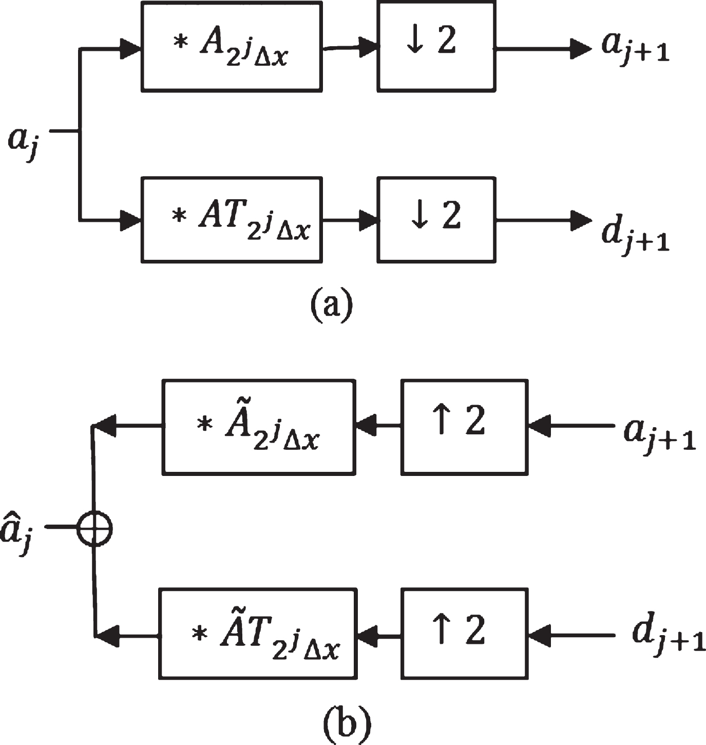
Representation of a fuzzy wavelet decomposition and reconstruction step where convolution, decimation and upsampling are denoted by ∗, ↓2 and ↑2, respectively.

3 Fuzzy wavelet thresholding

We consider the usual nonparametric model: $Y_{i} = f (i) + ɛ_{i}; i = 1, . . ., n$ (15) where Y₁, …, Y_n are observations, f is an unknown function to be recovered through the observations and $ɛ_{i} \overset{iid}{\sim} N (0, σ^{2})$ with unknown σ². To estimate f or denoise Y by fuzzy wavelet transform we propose a new method as follows:

Step 1: Decompose (Y₁, …, Y_n) by the fuzzy wavelet transform to obtain fuzzy wavelet coefficients up to level p using Equations (12) and (13);

Step 2: Threshold detail fuzzy wavelet coefficients obtained in Step 1;

Step 3: Perform the inverse fuzzy wavelet transform to obtain a denoised version of Y.

We apply our method to the example explained in Section 1. In Fig. 3, we can see the denoised version of Y_i = sin(2i) + ɛ_i based on the ordinary WD and the proposed method, i.e. Fuzzy Wavelet Denoising (FWD). In this figure, sin(2i), WD and FWD are denoted by dashed line, ‘∗’ and solid curve respectively. As it is evident, our method gives better results than WD.

Fig.3

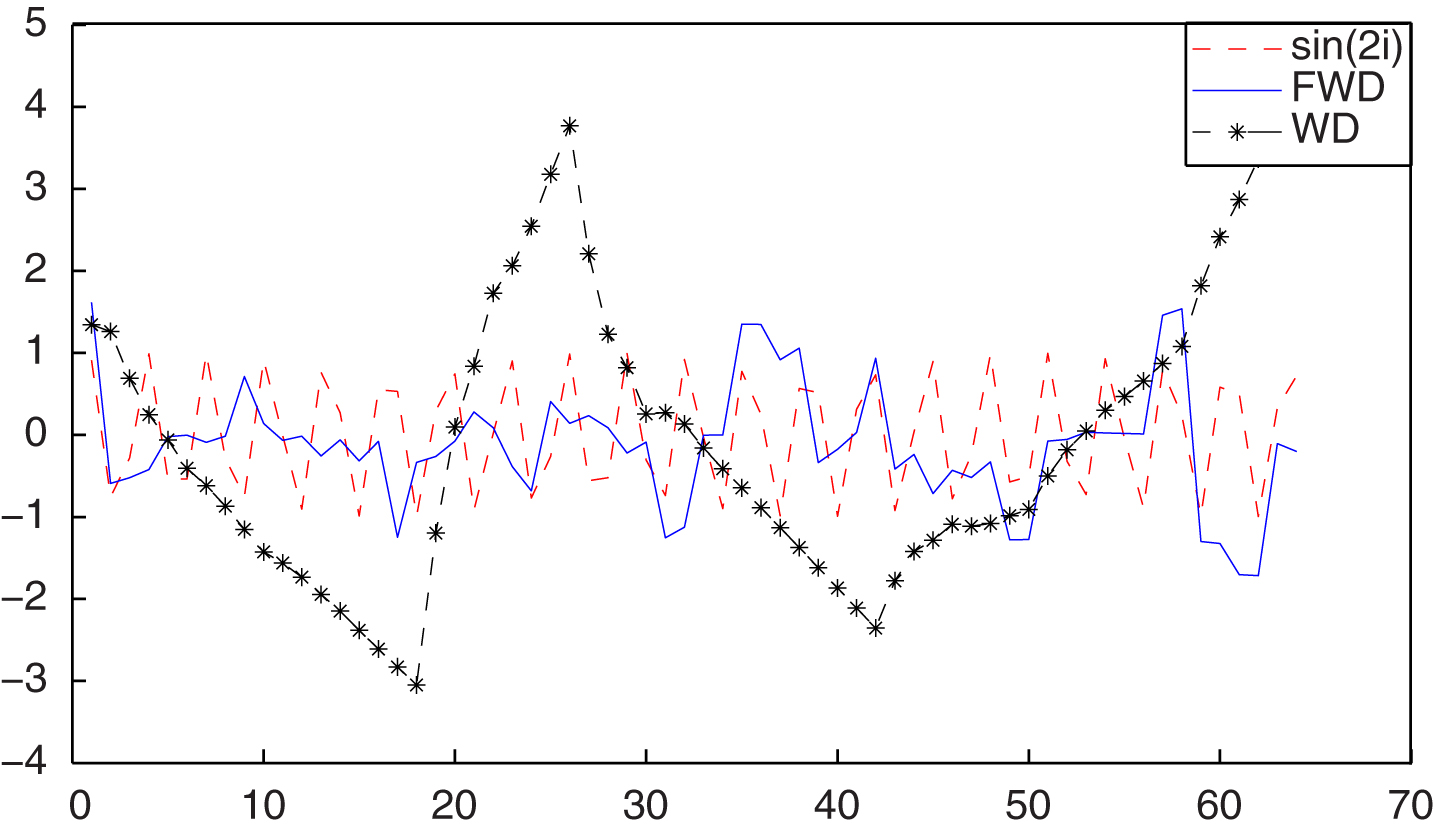
Fuzzy wavelet and ordinary wavelet denoising of Y_i = sin(2i) + ɛ_i. FWD fit (solid curve) and WD fit (‘∗’) and sin(2i) (dashed line).

In this example, since f is a periodic function, Fourier based denoising seems to be a good candidate. Figure 4 shows Fourier denoising (i.e., thresholding the Fourier coefficients by universal threshold) and our method for Y_i = sin(2i) + ɛ_i. In this figure, sin(2i), Fourier denoising and FWD fit are denoted by dashed line, ‘∗’ and solid curve respectively.

Fig.4

Fuzzy wavelet and Fourier denoising of Y_i = sin(2i) + ɛ_i. FWD fit (solid curve) and Fourier denoising fit (‘∗’) and sin(2i) (dashed line).

As it is shown in Figs. 3 and 4, our method works better than both Fourier denoising and ordinary wavelet denoising methods. The comparison of these three methods for 50 iterations is displayed in Section 4.

Let us provide more comments on step 2 of the FWD algorithm. When detail coefficients are small, it could be due to noise and can be ignored without affecting the estimation of f substantially. Thus, the idea of thresholding fuzzy wavelet coefficients is a way of cleaning out insignificant details. There are a variety of methods to choose a threshold denoted by λ. The threshold depends on the noise level and therefore, an estimate of the noise variance, σ². A robust estimator of σ (based on the median absolute deviation) is given by [3, Chapter 6]: $\hat{σ} = 1.4825 median (| d_{1} - median (d_{1}) |)$ (16) where d₁ is the vector of finest detail fuzzy wavelet coefficients.

We use the universal threshold where the name of the universal threshold given by Donoho and Johnstone [4] to $λ = \hat{σ} \sqrt{2 \log (n)}$ , where n is the sample size. For Gaussian white noise, the maximum noise level is smaller than $σ \sqrt{2 \log (n)}$ . The estimator $\hat{f}$ is obtained by preserving only detail fuzzy wavelet coefficients which are larger than λ. Similar to wavelet transform, fuzzy wavelet is also a linear transform.

Lemma 1. If the fuzzy partition of [a, b] (basic functions) is fixed, then the F-transform establishes a linear mapping from function space to $ℝ^{n}$ i.e., we have: $F_{n} [α f + β g] = α F_{n} [f] + β F_{n} [g]$ (17) for $α, β \in ℝ$ and arbitrary functions f and g given at points Z_n = {1, …, n}.

Proof 1. We denote k-th component of F_n [αf + βg] by F_k,αf+βg and k-th component of F_n [f] and F_n [g] by F_k,f and F_k,g, respectively. Based on Equation (7) for each component of F_n [αf + βg], we can write:

$\begin{matrix} F_{k, α f + β g} & = & \sum_{i = 1}^{n} (α f (i) + β g (i)) A_{k} (i) \\ = & \sum_{i = 1}^{n} α f (i) A_{k} (i) + \sum_{i = 1}^{n} β g (i) A_{k} (i) \\ = & α \sum_{i = 1}^{n} f (i) A_{k} (i) + β \sum_{i = 1}^{n} g (i) A_{k} (i) \\ = & α \sum_{i = 1}^{n} f (i) A (k - i) + β \sum_{i = 1}^{n} g (i) A (k - i) \\ = & α F_{k, f} + β F_{k, g} . \end{matrix}$ (18)

Therefore, based on this lemma, after decimation we have:

$\begin{matrix} 𝒟 (F_{n} [α f + β g]) \\ = {\sum_{i = 1}^{n} (α f (i) + β g (i)) A_{2 k} (i)}_{k = 1}^{\frac{n}{2}} \\ = {\sum_{i = 1}^{n} α f (i) A_{2 k} (i) + \sum_{i = 1}^{n} β g (i) A_{2 k} (i)}_{k = 1}^{\frac{n}{2}} \\ = 𝒟 (α F_{n} [f] + β F_{n} [g]) \\ = 𝒟 (α F_{n} [f]) + 𝒟 (β F_{n} [g]) \end{matrix}$ (19)

As it is mentioned before, scripfontD denotes the decimation operator. For j-th stage we have:

$\begin{matrix} 𝒟 ((α a_{j - 1} + β b_{j - 1}) * A_{2^{j - 1} △ x}) \\ = 𝒟 (α a_{j - 1} * A_{2^{j - 1} △ x} + β b_{j - 1} * A_{2^{j - 1} △ x}) \\ = 𝒟 (α a_{j - 1} * A_{2^{j - 1} △ x}) + 𝒟 (β b_{j - 1} * A_{2^{j - 1} △ x}) \\ = α a_{j} + β b_{j} \end{matrix}$ (20) where a_j and b_j are approximation fuzzy wavelet coefficients of the j-th stage decomposition of f and g, respectively. Therefore, fuzzy wavelet transform is also a linear transform: $θ_{i} = τ_{i} + ω_{i}, i = 1, \dots, n$ (21) where θ_i, τ_i and ω_i, denote fuzzy wavelet coefficients of Y_i, f (i) and ɛ_i, respectively.

The function A (x) in Equation (13) works as a weight in this transform since fuzzy wavelet characterizes some local characteristic of the original function. For instance, precise values of independent variables in nonparametric regression problem are factorized or fuzzified by a “closeness” relation like “approximately 2”, and precise values of dependent variables (nonparametric regression function values) are averaged to an approximate value. Therefore, the following theorem is established.

Theorem 1. Let $ɛ_{i} \overset{iid}{\sim} N (0, σ^{2})$ and {A_i} , i = 1, …, n, be basic functions on the domain of ɛ_i that satisfy all conditions described in Section 2. The detail fuzzy wavelet coefficients of ɛ_i is colored noise with $d_{j} = {d_{j, 1}, \dots, d_{j, \frac{n}{2^{j}}}} \sim N (0, Σ_{\frac{n}{2^{j}} \times \frac{n}{2^{j}}}^{j})$ where $Σ_{\frac{n}{2^{j}} \times \frac{n}{2^{j}}}^{j} = [σ_{l, m}^{j}]_{l, m}$ such that:

$\begin{matrix} σ_{l, m}^{j} & = & Cov (d_{j, l}, d_{j, m}) \\ = & \sum_{i = 1}^{\frac{n}{2^{j - 1}}} \sum_{k = 1}^{\frac{n}{2^{j - 1}}} {({AT}_{2^{j - 1} △ x} (2 l - 2^{j - 1} i)) \\ \times ({AT}_{2^{j - 1} △ x} (2 m - 2^{j - 1} k)) \\ Cov (a_{j - 1, i}, a_{j - 1, k})} \end{matrix}$ (22) for j-th stage.

Proof 2. Using Lemma 1, for the first stage, the transform of ɛ_i is F_n [ɛ] = [F₁, …, F_n] where: $F_{k} = \sum_{i = 1}^{n} ɛ_{i} {AT}_{k} (i) = \sum_{i = 1}^{n} ɛ_{i} AT (k - i)$ (23) for k = 1, …, n. Using the decimation operator, we have: $d_{1} = [d_{1, 1}, d_{1, 2}, \dots, d_{1, \frac{n}{2}}] = [F_{2}, F_{4}, \dots, F_{n}] .$ (24) In this case, the expectation of d₁, is computed as follows:

$\begin{matrix} 𝔼 (d_{1, m}) & = & 𝔼 (F_{2 m}) = 𝔼 (\sum_{i = 1}^{n} ɛ_{i} AT (2 m - i)) \\ = & \sum_{i = 1}^{n} AT (2 m - i) 𝔼 (ɛ_{i}) = 0 \end{matrix}$ (25)

For j-th stage, based on Equation (12) the mean of d_j,m is obtained as follows:

$\begin{matrix} 𝔼 (d_{j, m}) & = & 𝔼 (\sum_{i = 1}^{\frac{n}{2^{j - 1}}} a_{j - 1, i} {AT}_{2^{j - 1} △ x} (2 m - 2^{j - 1} i)) \\ = & \sum_{i = 1}^{\frac{n}{2^{j - 1}}} {AT}_{2^{j - 1} △ x} (2 m - 2^{j - 1} i) 𝔼 (a_{j - 1, i}) = 0 \end{matrix}$ (26) since a_0,i = ɛ_i. For next stages, each approximation coefficient is also a linear combination of fuzzy basic functions and approximation coefficients of the previous stage, therefore, $𝔼 (a_{j - 1, i}) = 0$ .

Also, the covariance of d_1,l and d_1,m is computed as follows:

$\begin{matrix} Cov (d_{1, l}, d_{1, m}) \\ = Cov (\sum_{i = 1}^{n} ɛ_{i} AT (2 l - i), \sum_{k = 1}^{n} ɛ_{k} AT (2 m - k)) \\ = \sum_{i = 1}^{n} \sum_{k = 1}^{n} (AT (2 l - i)) (AT (2 m - k)) Cov (ɛ_{i}, ɛ_{k}) \\ = \sum_{i = 1}^{n} (AT (2 l - i)) (AT (2 m - i)) Var (ɛ_{i}) \end{matrix}$ (27) for i = k, otherwise, Cov (ɛ_i, ɛ_k) =0. For j-th stage, the covariance of d_j,l and d_j,m is calculated as follows:

$\begin{matrix} Cov (d_{j, l}, d_{j, m}) \\ = Cov (\sum_{i = 1}^{\frac{n}{2^{j - 1}}} a_{j - 1, i} {AT}_{2^{j - 1} △ x} (2 l - 2^{j - 1} i), \\ \sum_{k = 1}^{\frac{n}{2^{j - 1}}} a_{j - 1, k} {AT}_{2^{j - 1} △ x} (2 m - 2^{j - 1} k)) \\ = \sum_{i = 1}^{\frac{n}{2^{j - 1}}} \sum_{k = 1}^{\frac{n}{2^{j - 1}}} {({AT}_{2^{j - 1} △ x} (2 l - 2^{j - 1} i)) \\ ({AT}_{2^{j - 1} △ x} (2 m - 2^{j - 1} k)) Cov (a_{j - 1, i}, a_{j - 1, k})} . \end{matrix}$ (28)

Since convolution is a linear mapping and all properties of normal distribution are preserved, hence, $d_{j} = {d_{j, 1}, \dots, d_{j, \frac{n}{2^{j}}}} \sim N (0, Σ_{\frac{n}{2^{j}} \times \frac{n}{2^{j}}}^{j})$ .

Since d_js are colored noise with a different variance in each level, we have to use level-dependent thresholding [9, 18]. It means that we estimate the variance of the noise based on detail coefficients of each level. We can calculate λ, the threshold of each level, through the estimator of the variance of the same level.

Figure 5 shows a scheme of our proposed method for one level decomposition.

Fig.5

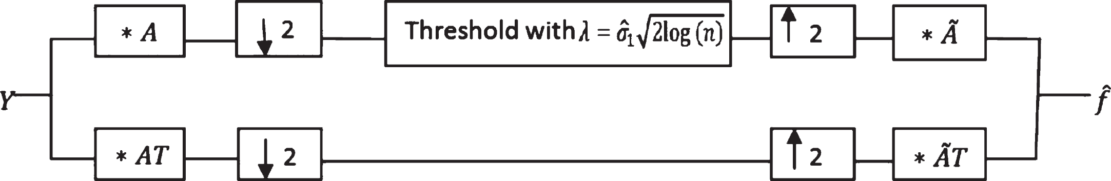
A scheme of our proposed method for one level decomposition.

4 Simulation results

In this section, we compare WD, FWD and Fuzzy denoising (F-transform denoising i.e,. thresholding the F-transform coefficients by universal threshold) through Mean Square Error (MSE) on simulations based on bench mark examples in the MATLAB software. MSE is estimated by: $R (k) = \frac{1}{n} \sum_{i = 1}^{n} (f_{i}^{k} - {\hat{f_{i}}}^{k})^{2}$ (29) where ${\hat{f_{i}}}^{k}$ is an estimator of $f_{i}^{k}$ over k-th iteration with sample size of n = 128. We estimate f_i by FWD, WD and Fuzzy denoising (shortly Fuzzy-D) and then compute R for each sample. We iterate this procedure 50 times and calculate the mean of R over the results of the 50 iterations. In the following example, a Gaussian noise $ɛ_{i} \overset{iid}{\sim} N (0, σ^{2})$ with σ² = 8 is added to signals. As we can see in Table 1, our proposed method works better than ordinary WD and Fuzzy-D methods. The best result in each row of the tables is bolded. In what follows, we use hard threshold and Daubechies wavelet with 2 vanishing moments.

Table 1

Mean(R) for FWD, WD and Fuzzy-D methods with sample size 128

Signal	FWD	WD	Fuzzy-D
Doppler	0.35	1.37	1.44
Quadchirp	0.71	1.61	1.67
Mishmash	2.00	2.37	2.55

Figures 6, 7 and 8 show denoised signals of noisy Doppler, Quadchirp and Mishmash respectively based on FWD, WD and Fuzzy-D methods for an iteration where ‘∘’, ‘-’, ‘∗’, ‘+’ and ‘▵’ represent Y, f, FWD, WD and Fuzzy-D, respectively. Although the SNR of all these examples is low, our method works well and outperforms WD and Fuzzy-D methods.

Fig.6

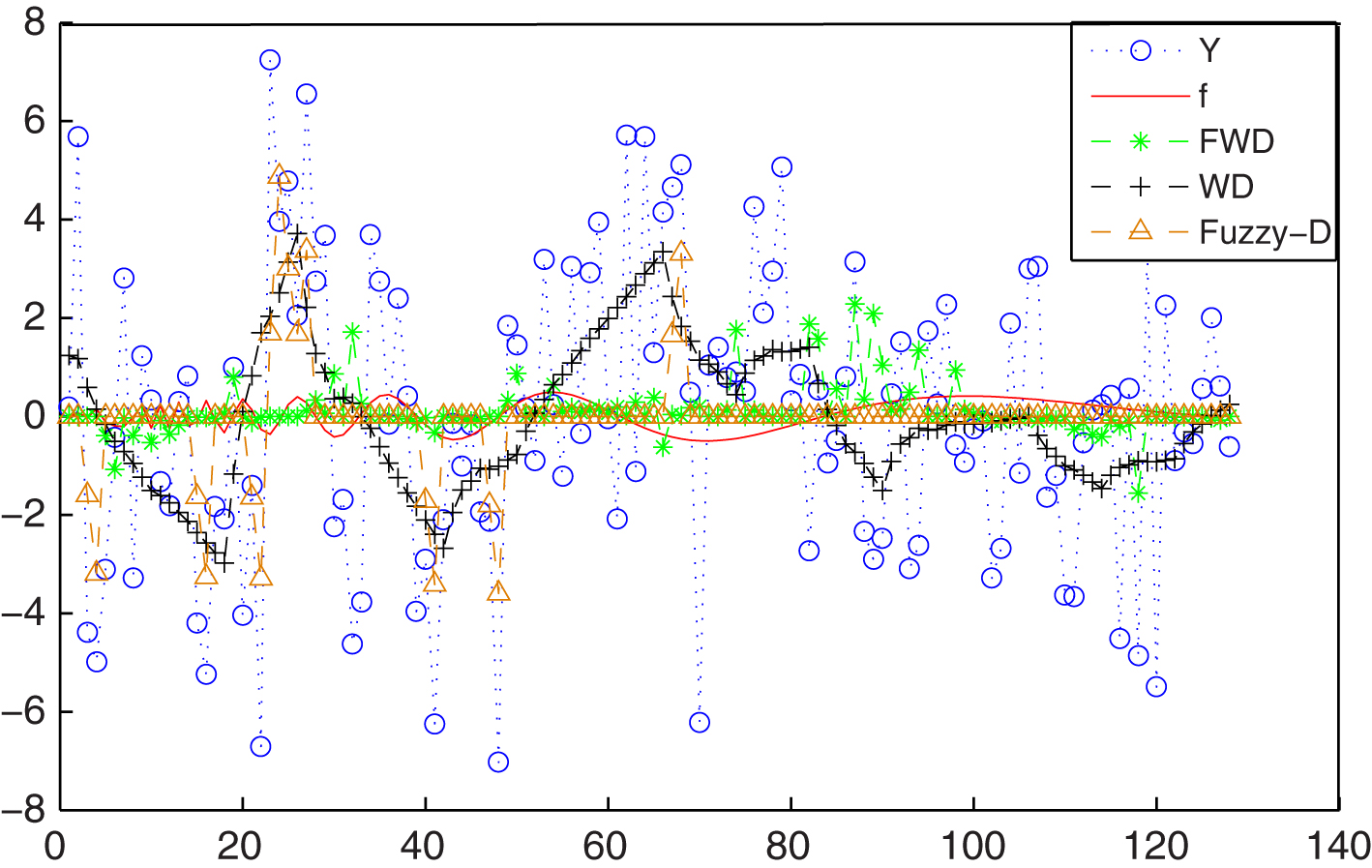
Denoising of Doppler signal contaminated by Gaussian noise using FWD, WD and Fuzzy-D methods. Y is denoted by ‘∘’, f by solid curve, corresponding FWD, WD and Fuzzy-D results by ‘∗’, ‘+’ and ‘▵’, respectively.

Fig.7

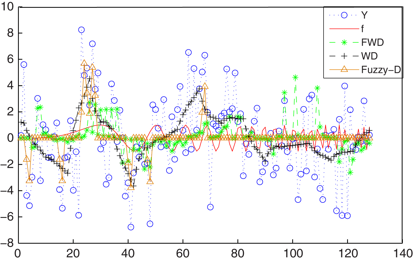
Denoising of Quadchirp signal contaminated by Gaussian noise using FWD, WD and Fuzzy-D methods. Y denoted by ‘∘’, f by solid curve, corresponding FWD, WD and Fuzzy-D results by ‘∗’, ‘+’ and ‘▵’, respectively.

Fig.8

Denoising of Mishmash signal contaminated by Gaussian noise using FWD, WD and Fuzzy-D methods. Y denoted by ‘∘’, f by solid curve, corresponding FWD, WD and Fuzzy-D results by ‘∗’, ‘+’ and ‘▵’, respectively.

In addition, in these examples we compar the standard deviation of R (denoted by std (R)) for FWD, WD and Fuzzy-D methods and their results are summarized in Table 2. The best performance corresponds to our method.

Table 2

std(R) for FWD, WD and Fuzzy-D methods with sample size 128

Signal	FWD	WD	Fuzzy-D
Doppler	0.29	0.69	0.69
Quadchirp	0.29	0.68	0.62
Mishmash	0.43	0.70	0.54

Figures 9, 10 and 11 show boxplots of R for Doppler, Quadchirp and Mishmash respectively based on FWD, WD and Fuzzy-D methods. As we can see in Figs. 9, 10 and 11, our method outperforms the other methods.

Fig.9

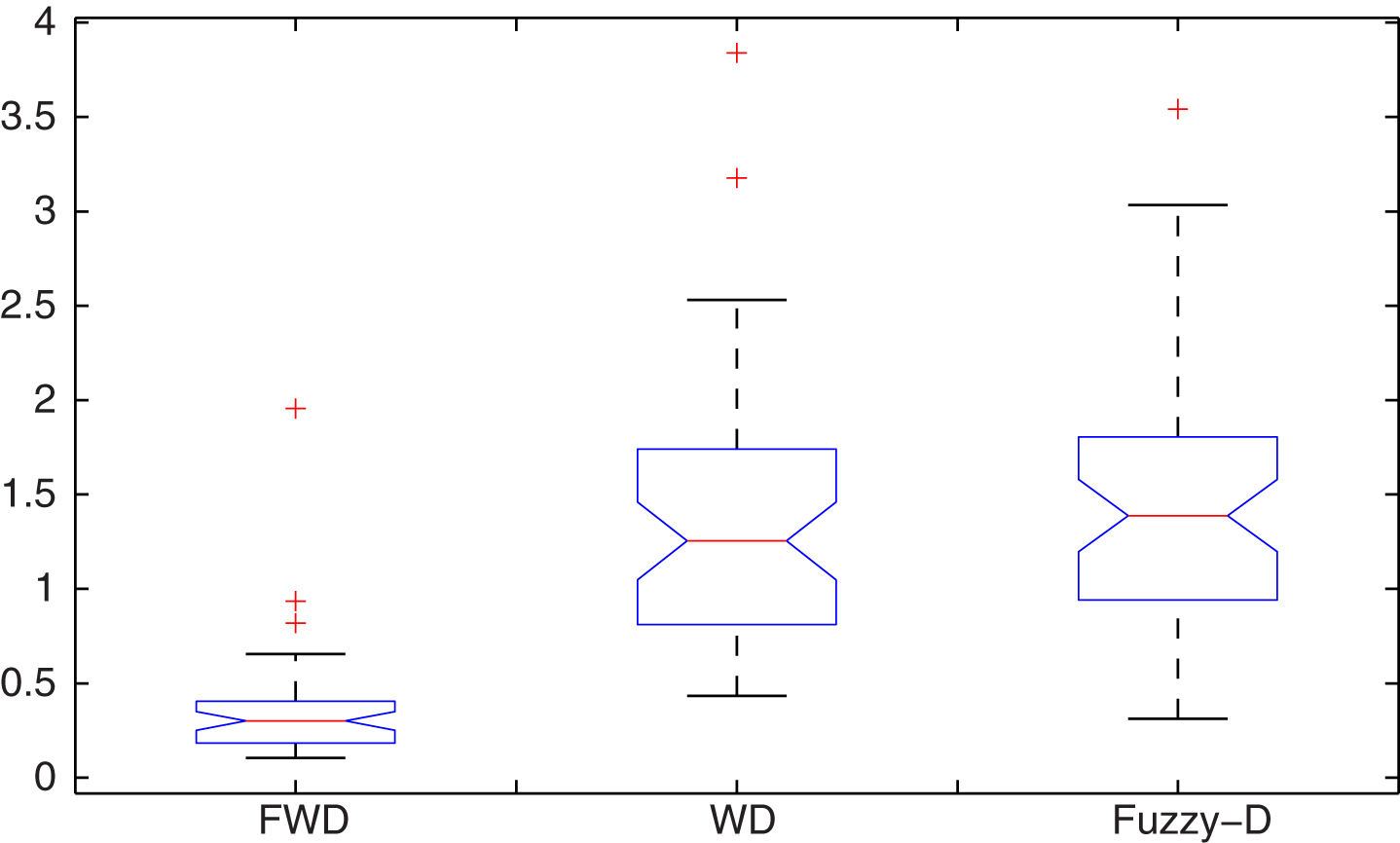
Boxplot of R for Doppler signal based on FWD, WD and Fuzzy-D methods.

Fig.10

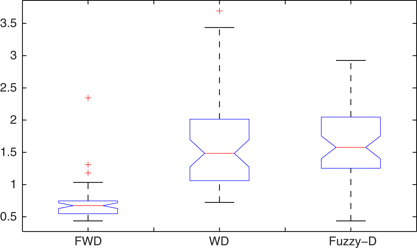
Boxplot of R for Quadchirp signal based on FWD, WD and Fuzzy-D methods.

Fig.11

Boxplot of R for Mishmash signal based on FWD, WD and Fuzzy-D methods.

To see more about the performance of the proposed method, we consider Doppler signal with different noise variances. In this case, the difference between the performance of the proposed method, WD and Fuzzy-D becomes more obvious when the noise variance is increased. The results are shown in Table 3.

Table 3

Mean(R) for FWD, WD and Fuzzy-D methods with sample size 128 of Doppler signal

σ ²	FWD	WD	Fuzzy-D
1	0.12	0.19	0.23
2	0.15	0.36	0.41
4	0.22	0.69	0.75
8	0.35	1.37	1.44
16	0.62	2.73	2.75

We also denoise an example which is mentioned in Section 3. This example is the noisy sinusoid i.e., Y_i = sin(2i) + ɛ_i for i = 1, …, 64. The performance of denoising methods, FWD, WD, Fuzzy-D and Fourier, over 50 iterations, are presented in Table 4.

Table 4

Mean(R) for FWD, WD, Fuzzy-D and Fourier denoising methods for sin(2i) + ɛ_i

FWD	WD	Fuzzy-D	Fourier Denoising
0.49	2.09	2.16	4.24

As it is shown the performance of the proposed method is far better than WD, Fuzzy-D and Fourier denoising methods. Figure 12 shows that $\bar{R} (n)$ for different methods against n, i.e. sample size, when J = 2. $\bar{R} (n)$ of our method converges to the constant value (its expectation) faster than other ones as n increasing.

Fig.12

Convergence of $\bar{R} (n)$ for our method against n for sin (2i) + ɛ_i.

5 Application of FWD to analysis of real audio data

We apply our method to different audio signals. The initial task is to improve the SNR by removing noise. We use the following definition of the SNR in db of a signal Y, $SNR (Y) = 20 {log}_{10} (\frac{max | Y |}{s (Y)})$ , where s (Y) is a robust estimator of the standard deviation of signal Y. This SNR is used in [12]. A greater SNR corresponds to the better method.

We consider two sets of data, a bird chirp signal and a musical signal. These audio signals are available examples in the MATLAB software with the name of chirp.mat and handel.mat, respectively. The bird chirp signal is used in [6].

To compare the performance of a method in speech signal processing, it is common to add some noises to the signal and then denoise it through different methods such as wavelet transform [1 , 20]. Therefore, we add a centered Gaussian white noise to the audio signals and compute SNR and R for 100 different initial SNR levels. The mean SNR and R for both FWD and WD are presented in Tables 5 and 6 for bird chirp and musical signal, respectively. Our method gives better results than WD method.

Table 5
Mean SNR and R for different SNR levels of the bird chirp signal

Measurement FWD WD

SNR 19.57 13.15

R 0.19 0.28

Measurement	FWD	WD
SNR	19.57	13.15
R	0.19	0.28

Table 6

Mean SNR and R for different SNR levels of the musical signal

Measurement	FWD	WD
SNR	19.66	13.61
R	0.1	0.2

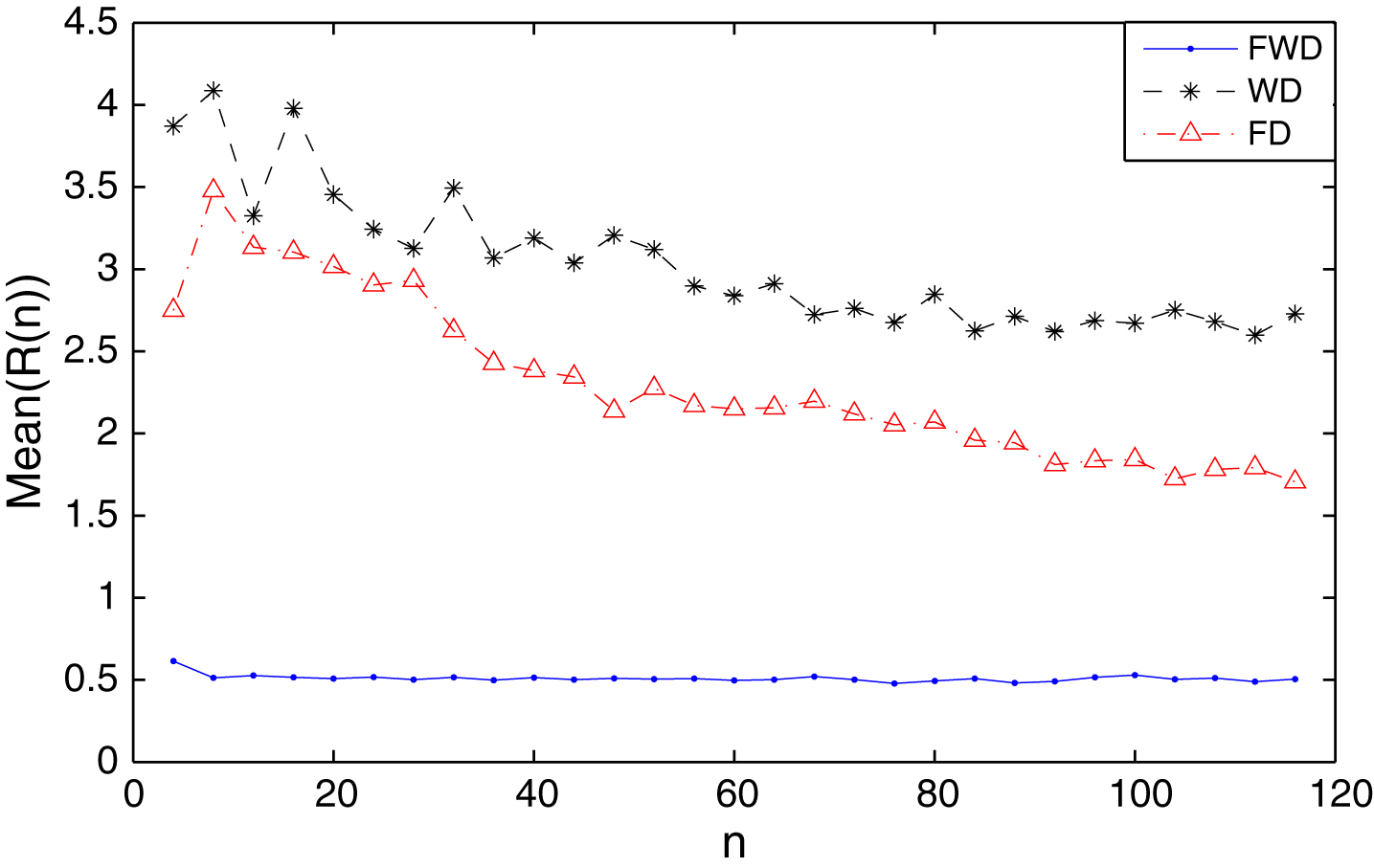
Figures 13 and 14 show the R and SNR of the denoised signals based on FWD and WD methods related to different SNR levels of the bird chirp signal, respectively. As we can see, the proposed method has better results.

Fig.13

R for FWD and WD methods for the bird chirp signal versus different SNR. FWD is denoted by ‘+’ and WD fit is denoted by ‘*’.

Fig.14

SNR for FWD and WD methods for the bird chirp signal versus different SNR. FWD is denoted by ‘+’ and WD fit is denoted by ‘*’.

Figures 15 and 16 show the R and SNR of the denoised signals based on FWD and WD methods related to different SNR levels of the musical signal, respectively.

Fig.15

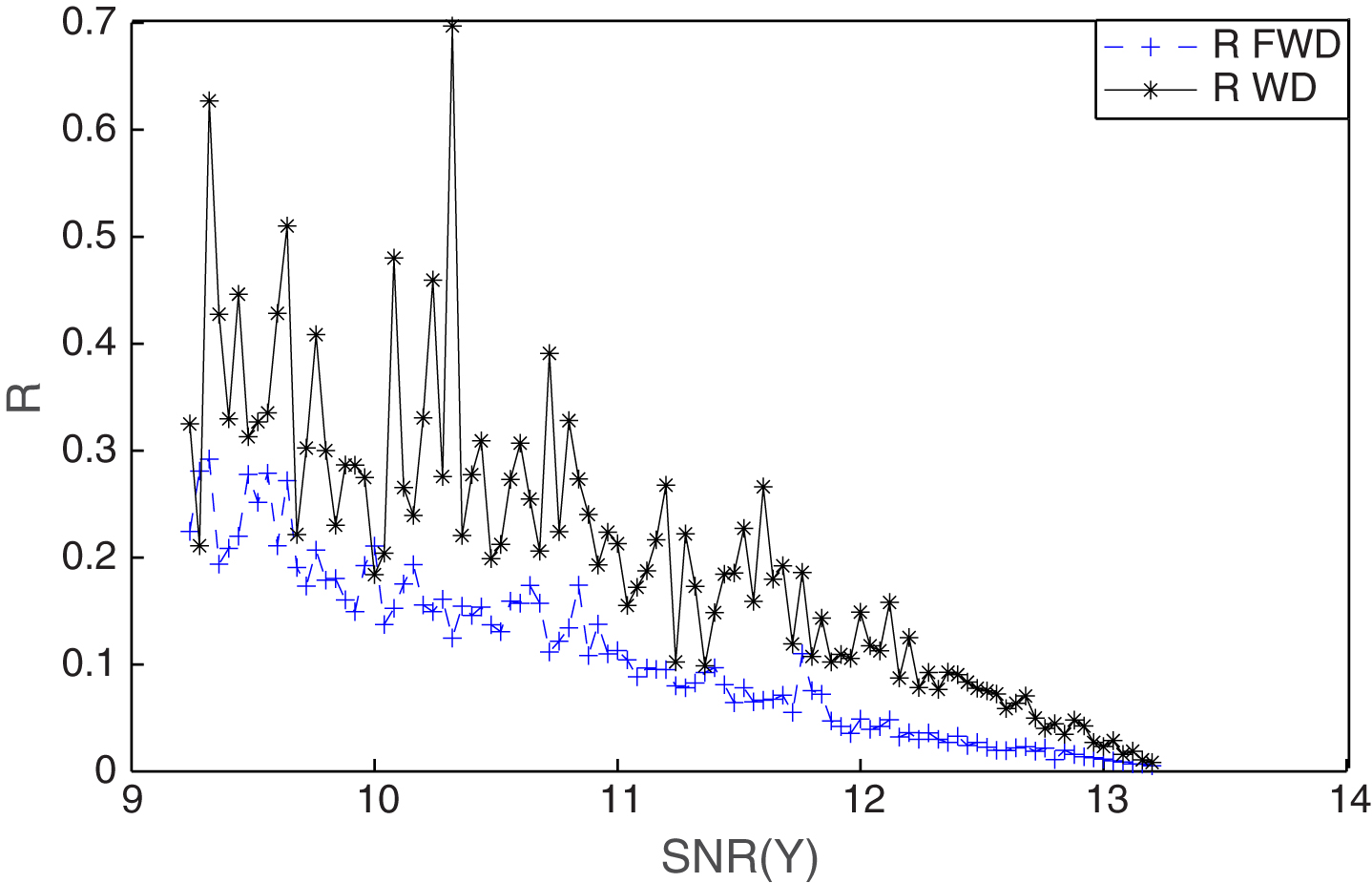
R for FWD and WD methods for different SNR of the musical signal. FWD is denoted by ‘+’ and WD fit is denoted by ‘*’.

Fig.16

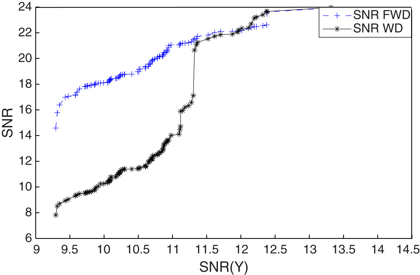
SNR for FWD and WD methods for different SNR levels of the musical signal. FWD is denoted by ‘+’ and WD fit is denoted by ‘*’.

As it is shown in Figs. 13, 14, 15 and 16, FWD method has better performance than WD method and FWD method is less sensitive to the change of the SNR of real data.

6 Conclusions

In this paper, we proposed a new fuzzy wavelet denoising method and compared it with ordinary wavelet denoising and fuzzy denoising methods. The new method is based on fuzzy wavelet transform and outperforms the other methods when it is applied to two different audio datasets as well as simulated data. For data with irregular pattern or small SNR, the difference of performance among three methods, FWD, WD and Fuzzy denoising, becomes more important. This fact shows the stability of the proposed method. For future work, we can work on non-equidistant data.

Acknowledgments

We would like to thank the editor and two anonymous referees for their valuable comments and suggestions.

References

Aicha

A.B.

and Jebara

S.B.

, Reduction of musical residual noise using perceptual tools with classic speech denoising techniques, Signal, Image and Video Processing6(1) (2012), 85–97.

JaiShankar

and Duraiswamy

, Audio denoising using wavelet transform, International Journal of Advances in Engineering & Technology2(1) (2012), 419–425.

Vidakovic

, Statistical Modeling by Wavelets. Wiley, New York, 1999.

Donoho

D.L.

and Johnstone

I.M.

, Ideal spatial adaptation by wavelet shrinkage, Biometrika81 (1994), 425–455.

, Cai

and Zhang

, Wind power prediction interval estimation method using wavelet-transform neuro-fuzzy network, Journal of Intelligent & Fuzzy Systems29 (2015), 2439–2445.

Krim

, Tucker

, Mallat

and Donoho

, On denoising and best signal representation, IEEE Transactions on Information Theory45(7) (1999), 2225–2238.

Agarwal

, Singh

, Rani

and Mittal

A.P.

, Hardware efficient denoising system for real EOG signal processing, Journal of Intelligent & Fuzzy Systems32(4) (2017), 2857–2862.

Beg

and Aamir

K.M.

, Fuzzy wavelets, The Journal of Fuzzy Mathematics21(3) (2013), 623–638.

Johnstone

I.M.

and Silverman

B.W.

, Wavelet threshold estimators for data with correlated noise, Journal of the Royal Statistical Society: Series B (Statistical Methodology)59(2) (1997), 319–351.

10.

Perfilieva

and Hodakova

, Fuzzy and Fourier transforms, 7th Conference of the European Society for Fuzzy Logic and Technology, Aix-les-Bains, France, 2011, pp. 452–456.

11.

Perfilieva

, Fuzzy transforms: Theory and applications, Fuzzy Sets and Systems157 (2006), 993–1023.

12.

Aminghafari

, Cheze

and Poggi

J.-M.

, Multivariate denoising using wavelets and principal component analysis, Computational Statistics & Data Analysis50 (2006), 2381–2398.

13.

Misiti

, Misiti

, Oppenheim

and Poggi

J.-M.

, Wavelets and their Applications, ISTE, London, 2007.

14.

Pan

, Yan

, Tu

and Jiang

, Fuzzy control and wavelet transform-based energy management strategy design of a hybrid tracked bulldozer, Journal of Intelligent & Fuzzy Systems29 (2015), 2565–2574.

15.

Weeks

and Bayoumi

, Discrete wavelet transform: Architectures, design and performance issues, Journal of VLSI Signal Processing Systems for Signal, Image and Video Technology35(2) (2003), 155–178.

16.

Kanirajan

and Kumar

V.S.

, Wavelet-based power quality disturbances detection and classification using RBFNN and fuzzy logic, International Journal of Fuzzy Systems17(4) (2015), 623–634.

17.

Yang

, Yang

, Gai

and Chen

, Block thresholding image denoising with dual-tree complex wavelet transform, Journal of Intelligent & Fuzzy Systems30(6) (2016), 3197–3207.

18.

Chen

S.H.

and Wang

J.F.

, Speech enhancement using perceptual wavelet packet decomposition and teager energy operator, Journal of VLSI Signal Processing Systems for Signal, Image and Video Technology36(2) (2004), 125–139.

19.

Jha

S.K.

and Yadava

R.D.S.

, Denoising by singular value decomposition and its application to electronic nose data processing, IEEE Sensors Journal11(1) (2011), 35–44.

20.

Bruni

, Piccoli

and Vitulano

, A fast computation method for time scale signal denoising, Signal, Image and Video Processing3(1) (2009), 63–83.