Fractional Jacobi operational matrix for solving Fuzzy Fractional Differential Equation 1

Abstract

In this paper, we have researched fractional Jacobi operational matrix for solving Fuzzy Linear Fractional Differential Equation of order 0 < ν < 1. By using fractional Jacobi operational matrix, it is to reduce the problem which obtain the approximative solution of Fuzzy Linear Fractional Differential Equation to solving of a system of Fuzzy Linear Algebraic Equation. We improved the accuracy of the numerical approximation of the solution by using fractional-order Jacobi functions and are verified by some examples.

Keywords

Fuzzy fractional differential equation fractional-order Jacobi functions Caputo-type fuzzy fractional derivative

1 Introduction

The application of fractional differential equations (FDEs) are extending to many areas such as control engineering [1], diffusion equations [2], signal processing [3], electromagnetism [4]. Recently many researchers have an interest in theory of the existence and uniqueness of FDEs [5 –7]. The problem that obtain the numerical solution of FDEs is important, but it is difficult to obtain exact solution of FDEs. The predictor-corrector method [8], Adomian’s decomposition method [9], variational iteration method [10] and homotopy analysis method [11] are typical methods.

The orthogonal functions is one of strong tools for obtain the numerical solution of high accuracy of FDEs. The advantage of this method is to reduce the problem that obtain the numerical solution of FDEs to the problem that obtain the solution of a system of algebraic equation. Specially in the case of linear fractional differential equation is to reduce the problem that obtain the solution of a system of linear algebraic equation. The operation matrix of orthogonal functions have supported the numerical solution methods for solving FDEs with the initial and boundary condition such as Chebyshev spectral method [12, 13], Laguerre operational matrices [14], fractional Legendre orthogonal functions [15] and Jacobi polynomials [16 –18]. Doha et al. [17, 18] presented the spectral tau and collocation method for solving linear and nonlinear FDEs by using Jacobi polynomials. Recently Bhrawy et al. [19] raised shifted fractional Jacobi functions which generalize shifted Jacobi polynomials in [17, 18] and improved the accuracy of numerical solution of Caputo-type fractional differential equation by using proposed method.

The study of fuzzy fractional differential equation occasionally (FFDEs) is expressed for the sufficient mathematical modeling of the real world phenomenon with uncertainties or vagueness. These problems were introduced by Anastassiou [24] and Hukuhara [25]. Bede and Gal [27] is introduced the strongly generalized differentiability which generalize the H-derivative and Chehabi et al. [38] studied the concreted solutions of fuzzy linear fractional differential equations.

Recently researchers proposed several attempts for numerical methods of FFDEs. Mazandarani et al. [20] obtained approximation solution of FFDEs by using modified Euler method under Caputo-type’s differentiability and Salahshour et al. [21] proposed fuzzy Laplace transform for solving FFDEs under Riemann-Liouville’s differentiability. Prakasha et al. [37] proposed the method using Banach fixed point theorem and Allahviranloo et al. [36] obtained analytical solution of FFDEs. Ahmadian et al. [22, 23] obtained numerical solution of the initial value problem of fuzzy linear FDEs by using Jacobi and Legendre operational matrix and Armand et al. [39] introduced the fuzzy variation iteration method.

In this paper, we generalized shifted fractional Jacobi functions for solving fuzzy linear fractional differential equation of order 0 < ν < 1 under Caputo-type differentiability and proposed the method to obtain sufficient approximation of fuzzy function by using shifted fractional Jacobi functions. The errors of numerical solutions obtained by using fractional Jacobi operational matrix presented were shown smaller than the errors of numerical solutions obtained by using Jacobi operational matrix for several examples.

This paper constructed as follows. In Section 2, we described some properties of fuzzy calculus and fraction calculus. A few properties of fuzzy fractional Caputo type derivative and shifted fractional-order Jacobi functions is described in Section 3. Section 4 described use of shifted fractional Jacobi functions for obtain the numerical solution of fuzzy linear fractional differential equation. In Section 5 are presented the numerical solutions result of some examples of fuzzy linear fractional differential equations and are described some conclusions in Section 6.

2 Preliminaries

2.1 Fuzzy calculus

Let us denote by $E$ the class of fuzzy subsets u of the real axis $ℝ$ (i. e. $u : ℝ \to [0, 1]$ satisfying the following properties):

u is upper semi-continuous,

u is fuzzy convex,

u is normal, i. e., $\exists x_{0} \in ℝ$ , u (x₀) =1,

supp $u = {x \in ℝ$ | u (x) >0} is the support of the u, and its closure cl(supp u) is compact.

Then $E$ is called the space of fuzzy real numbers and any $u \in E$ is called fuzzy real number. The r-level set of a fuzzy number $u \in E$ , 0 ≤ r ≤ 1, denoted by [u] ^r, is defined as $[u]^{r} = {\begin{matrix} {x \in ℝ | u (x) \geq 0} & if 0< r≤ 1, \\ cl (supp u) & if r=0 . \end{matrix}$

It is obvious that the r-level set of a fuzzy number is a closed and bounded interval [ $u_{-}^{r}$ , $u_{+}^{r}$ ] on $ℝ$ , where $u_{-}^{r}$ denotes the left-hand endpoint of [u] ^r and $u_{+}^{r}$ denotes the right-hand endpoint of [u] ^r. The addition and scaler multiplication of fuzzy number in $E$ are defined as $[u \oplus v]^{r} = [u_{-}^{r} + v_{-}^{r}, u_{+}^{r} + v_{+}^{r}],$ $[λ ⊙ u]^{r} = [λ u_{-}^{r}, λ u_{+}^{r}], λ \geq 0$ .

The metric D on $E$ ( $D : E \times E \to ℝ_{+} ⋃ 0)$ are defined so-called Hausdorff distance as follows: $D (u, v) = sup_{r \in [0, 1]} max {| u_{-}^{r} - v_{-}^{r} |, | u_{+}^{r} - v_{+}^{r} |} .$

Definition 1. [24] Let f and g be the two fuzzy-number-valued functions on the interval [a, b], i. e., $f, g : [a, b] \to E$ . The uniform distance between fuzzy-number-valued functions is defined by $D^{*} (f, g) = sup_{x \in [a, b]} D (f (x), g (x)) .$ (1)

Definition 2. [25] Let $x, y \in E$ . If there exists $z \in E$ such that x = y ⊕ z, then z is called the H-difference of x and y, and it is denoted by x ⊖ y.

Definition 3. [26] Given two fuzzy numbers $u, v \in E$ , the generalized Hukuhara difference (gH-difference for short) is the fuzzy number w, if it exists, such that $[u \underset{g}{⊖} v] = w \Leftrightarrow {\begin{matrix} (1) & u = v + w or \\ (2) & v = u - w \end{matrix}$

Although Hukuhara difference is not exist, generalized Hukuhara difference is sure to exist.

Proposition 1. [26] For any fuzzy numbers $u, v \in E$ , the g-difference $u \underset{g}{⊖} v$ exists and it is a fuzzy number.

Definition 4. [27] Let $f : (a, b) \to E$ and x₀ ∈ (a, b). We say that f is strongly generalized differential at x₀. If there exists an element $f^{'} (x) \in E$ , such that

∀h > 0 sufficiently small, ∃f (x₀ + h) ⊖ f (x₀), ∃f (x₀) ⊖ f (x₀ - h) and the limits (in the metric D) $\begin{matrix} f^{'} (x_{0}) & = & lim_{h \to 0^{+}} \frac{f (x_{0} + h) ⊖ f (x_{0})}{h} \\ = & lim_{h \to 0^{+}} \frac{f (x_{0}) ⊖ f (x_{0} - h)}{h}, \end{matrix}$

∀h > 0 sufficiently small, ∃f (x₀) ⊖ f (x₀ + h), ∃f (x₀ - h) ⊖ f (x₀) and the limits (in the metric D) $\begin{matrix} f^{'} (x_{0}) & = & lim_{h \to 0^{+}} \frac{f (x_{0}) ⊖ f (x_{0} + h)}{- h} \\ = & lim_{h \to 0^{+}} \frac{f (x_{0} - h) ⊖ f (x_{0})}{- h} . \end{matrix}$

Remark 1. f is so-called (1)-differentiable on (a, b), if f is differentiable in the sense (i) of Definition 4 and also f is (2)-differentiable on (a, b), if f is differentiable in the sense (ii) of Definition 4.

Theorem 1. [28] Let $F : (a, b) \to E$ be a fuzzy-valued function and denote [F (t)] ^r = [f_r (t), g_r (t)], for each r ∈ [0, 1]. Then:

If F is (1)-differentiable, then f_r (t) and g_r (t) are differentiable functions and $[F^{'} (t)]^{r} = [f_{r}^{'} (t), g_{r}^{'} (t)] .$

If F is (2)-differentiable, then f_r (t) and g_r (t) are differentiable functions and $[F^{'} (t)]^{r} = [g_{r}^{'} (t), f_{r}^{'} (t)] .$

Definition 5. [29] Let $f : [a, b] \to E$ . We say that f fuzzy-Riemann integrable to $I \in E$ , if for any ɛ > 0, there exists δ > 0 such that for any division P = {[u, v]; ζ} of [a, b] with the norms Δ (P) < δ, we have $D (\sum_{p}^{*} (u - v) \circ f (ζ), I) < ɛ,$ where ∑^* means addition with respect to ⊕ in $E$ , $I : = (FR) \int_{a}^{b} f (x) dx .$

We also call an f as above (FR)-integrable.

Definition 6. [30] Consider the n × n linear system of equations: ${\begin{matrix} a_{11} x_{1} + a_{12} x_{2} + \dots + a_{1 n} x_{n} = y_{1} \\ a_{21} x_{1} + a_{22} x_{2} + \dots + a_{2 n} x_{n} = y_{2} \\ ⋮ \\ a_{n 1} x_{1} + a_{n 2} x_{2} + \dots + a_{nn} x_{n} = y_{n} \end{matrix}$ (2)

The matrix form of the above equations is $AX = Y,$ (3) where the coefficient matrix A = (a_ij), 1 ≤ i, j ≤ n is a crisp n × n matrix and $y_{i} \in E$ , 1 ≤ i ≤ n. This system is called a fuzzy linear system (FLS).

To solve fuzzy linear systems, can refer to [35].

2.2 Fractional calculus

Definition 7. [32] The Riemann-Liouville fractional integral operator of order ν (ν ≥ 0) is defined as $(I^{ν} f) (x) = \frac{1}{Γ (ν)} \int_{0}^{x} \frac{f (t)}{(x - t)^{1 - ν}} dt, ν > 0, x > 0,$

Definition 8. [32] The Caputo fractional derivatives of order ν is defined as $^{c} D^{ν} f (x) = \frac{1}{Γ (m - ν)} \int_{0}^{x} (x - t)^{m - ν - 1} f^{(m)} (t) dt,$ where ^cD^m is the classical differential operator of order m and m - 1 < ν ≤ m, x > 0,.

For the Caputo derivative, we have:

$\begin{matrix} ^{c} D^{ν} C & = & 0 (C is a constant),^{} \\ ^{c} D^{ν} x^{β} & = & {\begin{matrix} 0, & for β \in ℕ_{0}, β < ⌈ ν ⌉, \\ \frac{Γ (β + 1)}{Γ (β + 1 - ν)} x^{β - ν}, & \begin{matrix} for β \in ℕ_{0}, β \geq ⌈ ν ⌉ \\ or β \notin ℕ, β > ⌊ ν ⌋ . \end{matrix} \end{matrix} \end{matrix}$ (4)

The ceiling function ⌈ν⌉ is used to denote the smallest integer greater than or equal to ν, and the floor function ⌊ν⌋ to denote the largest integer less than or equal to ν. Also $ℕ = {1, 2, \dots}$ and $ℕ_{0} = {0, 1, 2, \dots}$ .

3 Fuzzy fractional Caputo’s derivative and shifted fractional-order Jacobi function

3.1 Some properties of Fuzzy fractional Caputo-type derivative

At first, we introduce some notation for understand this paper [22]

$L_{p} (I, E)$ , 1≤ p ≤ ∞ is the set of all fuzzy-valued measurable functions f on I where the norm is defined by $∥ f ∥_{p} = (\int_{0}^{1} (d (f (t), 0))^{p} dt)^{\frac{1}{p}}$

$C (I, E)$ is a space of fuzzy-valued functions, which are continuous on I.

$AC (I, E)$ is a space of all fuzzy-valued functions, which are absolutely continuous on I, where I = [0, 1].

Definition 9. [38] Let $f \in C (I, E) ⋂ L_{1} (I, E)$ . The fuzzy Riemann-Liouville integral of fuzzy-valued function f is defined as follow $(I_{0 +}^{ν} f) (x) = \frac{1}{Γ (ν)} \int_{0}^{x} (x - t)^{ν - 1} f (t) dt, x > 0,$ where 0 < ν ≤ 1.

Definition 10. [34] Let $f \in C (I, E) ⋂ L_{1} (I, E)$ is a fuzzy-valued function, then f is said to be Caputo’s fuzzy differentiable at x when $(^{c} D_{0 +}^{ν} f) (x) = \frac{1}{Γ (1 - ν)} \int_{0}^{x} (x - t)^{- ν} f^{'} (t) dt,$ where 0 < ν ≤ 1.

Definition 11. [34] Let $f \in C (I, E) ⋂ L_{1} (I, E)$ and x₀ ∈ I and $Φ (x) = \frac{1}{Γ (1 - ν)} \int_{0}^{x} \frac{f (t) ⊖ \sum_{k = 0}^{1} \frac{t^{k}}{k!} f_{0}^{(k)}}{(x - t)^{ν}} dt$ , where $f_{0}^{(k)} = \frac{d^{k} f (x)}{{dx}^{k}} |_{x = 0}$ . We say that f (x) is fuzzy Caputo fractional differentiable of order 0 < ν ≤ 1 at x₀, if there exists an element $(^{c} D_{0 +}^{ν} f) (x_{0}) \in C (I, E)$ such that for h > 0 sufficiently near zero on either; $\begin{matrix} 1) (^{c} D_{0 +}^{ν} f) (x_{0}) & = & lim_{h \to 0^{+}} \frac{Φ (x_{0} + h) ⊖ Φ (x_{0})}{h} \\ = & lim_{h \to 0^{+}} \frac{Φ (x_{0}) ⊖ Φ (x_{0} - h)}{h}, \end{matrix}$ or $\begin{matrix} 2) (^{c} D_{0 +}^{ν} f) (x_{0}) & = & lim_{h \to 0^{+}} \frac{Φ (x_{0}) ⊖ Φ (x_{0} + h)}{- h} \\ = & lim_{h \to 0^{+}} \frac{Φ (x_{0} - h) ⊖ Φ (x_{0})}{- h} . \end{matrix}$

Remark 2. [31] A fuzzy-valued function f is ^c [1 - ν]-differentiable, if it is differentiable as in the Definition 11, case 1, and it is ^c [2 - ν]-differentiable, if it is differentiable as in the Definition 11, case 2.

Theorem 2. [31] Let us assume that $f \in C (I, E)$ , then we have the following: $(I_{a +}^{ν}^{c} D_{a +}^{ν} f) (x) = f (x) ⊖ f (a), 0 < ν < 1,$ when f is ^c [1 - ν]-differentiable and $(I_{a +}^{ν}^{c} D_{a +}^{ν} f) (x) = - f (a) ⊖ (- f (x)), 0 < ν < 1,$ when f is ^c [2 - ν]-differentiable.

Theorem 3. [31] Let 0 < r < 1 and $f \in AC (I, E)$ , then the fuzzy Caputo derivative can be stated using the fuzzy fractional Riemann-Liouville integral operator as follows: $(^{c} D_{a +}^{ν} f)^{r} (x) = [(I_{a +}^{1 - ν} Df)_{-}^{r} (x), (I_{a +}^{1 - ν} Df)_{+}^{r} (x)],$ when f is ^c [1 - ν]-differentiable and $(^{c} D_{a +}^{ν} f)^{r} (x) = [(I_{a +}^{1 - ν} Df)_{+}^{r} (x), (I_{a +}^{1 - ν} Df)_{-}^{r} (x)],$ when f is ^c [2 - ν]-differentiable.

3.2 Shifted fractional Jacobi orthogonal function

The analytic form of the shifted Jacobi polynomials $P_{n}^{(α, β)} (x)$ of degree i is acquired by [17, 22]

$\begin{matrix} P_{n}^{(α, β)} (x) \\ = \sum_{k = 0}^{n} E_{k}^{(α, β, n)} x^{k}, n = 0, 1, 2, \dots \\ E_{k}^{(α, β, n)} \\ = \frac{(- 1)^{n - k} Γ (n + β + 1) Γ (n + k + α + β + 1)}{Γ (k + β + 1) Γ (n + α + β + 1) (n - k)! k!} . \end{matrix}$ (5)

The shifted fractional-order Jacobi function is defined by [19] $P_{n}^{(α, β, λ)} (x) = \sum_{k = 0}^{n} E_{k}^{(α, β, n)} x^{λ k}, n = 0, 1, 2, \dots$ where x ∈ [0, 1] = I, 0 < λ < 1. It is clearly following properties as Jacobi orthogonal functions. $\begin{matrix} P_{n}^{(α, β, λ)} (0) & = & (- 1)^{n} \frac{Γ (n + β + 1)}{Γ (β + 1) n!}, \\ P_{n}^{(α, β, λ)} (1) & = & \frac{Γ (n + α + 1)}{Γ (α + 1) n!} . \end{matrix}$

Now let w^(α,β,λ) (x) = λx^λβ+λ-1 (1 - x^λ) ^α, α, β > -1. Then the fractional-order Jacobi functions form a complete $L_{w^{(α, β, λ)}}^{2} (I)$ -orthogonal system, i.e., $\int_{I} P_{i}^{(α, β, λ)} (x) P_{j}^{(α, β, λ)} (x) w^{(α, β, λ)} (x) dx = h_{j}^{(α, β)} δ_{ij},$ where δ_ij is Kronecker function and $h_{j}^{(α, β)} = \frac{Γ (j + α + 1) Γ (j + β + 1)}{(2 j + α + β + 1) Γ (j + 1) Γ (j + α + β + 1)} .$

The finite-dimensional fractional-polynomial space is defined such as $F_{N} = span {P_{n}^{(α, β, λ)} (x) : 0 \leq n \leq N} .$

Any $u \in L_{w^{(α, β, λ)}}^{2} (I)$ can de expanded as

$\begin{matrix} u (x) & = & \sum_{j = 0}^{\infty} {\hat{u}}_{j} P_{j}^{(α, β, λ)} (x), \\ {\hat{u}}_{j} & = & \int_{I} u (x) P_{j}^{(α, β, λ)} (x) w^{(α, β, λ)} (x) dx . \end{matrix}$ (6)

Theorem 4. [19] Suppose that D^kλu (x) ∈ C [0, 1] for k = 0, 1, ⋯, N - 1, (3 +2N + β) λ > 0. If u_N (x) is the best approximation to u (x) from F_N, then the error bound is presented as follows

$\begin{matrix} ∥ u (x) - u_{N} (x) ∥_{w} \\ \leq \frac{E_{λ}}{Γ ((N + 1) λ + 1)} \\ \times \sqrt{\frac{Γ (1 + α) Γ (3 + 2 N + β)}{Γ (4 + 2 N + α + β)}} . \end{matrix}$ (7) where E_λ ≥ |D^(N+1)λu (x) |, x ∈ I.

Theorem 5. [19] The fractional derivative of order ν (0 < ν ≤ 1) in the Caputo sense for the Shifted fractional-order Jacobi functions(SFJFs) is given by $D^{ν} P_{i}^{(α, β, λ)} (x) = \sum_{j = 0}^{N} S_{ν} (i, j, α, β, λ) P_{j}^{(α, β, λ)} (x),$ where $\begin{matrix} S_{ν} (i, j, α, β, λ) \\ = \sum_{k = 1}^{i} \frac{Γ (λ k + 1) Γ (α + 1)}{h_{j}^{(α, β)} Γ (λ k - ν + 1)} E_{k}^{(α, β, i)} \\ \times \sum_{s = 0}^{j} \frac{Γ (1 + k + s + β - \frac{ν}{λ})}{Γ (2 + k + s + α + β - \frac{ν}{λ})} E_{s}^{(α, β, j)} . \end{matrix}$

4 Application of shifted fractional Jacobi operational matrix

4.1 Approximation of fuzzy valued function by shifted fractional Jacobi function

Definition 12. The fuzzy-valued function y (x) is approximated following as by the shifted fractional-order Jacobi functions $P_{i}^{(α, β, λ)}$ on [0, 1] and for 0 < λ < 1, $y \in C (I, E) ⋂ L_{1} (I, E)$ : $y (x) = \sum_{i = 0}^{+ \infty}^{*} θ_{i} ⊙ P_{i}^{(α, β, λ)} (x), i = 0, 1, \dots,$ (8) where fuzzy coefficient θ_i is given $θ_{i} = \frac{1}{h_{j}^{(α, β)}} \int_{0}^{1} P_{i}^{(α, β, λ)} (x) ⊙ y (x) ⊙ w^{(α, β, λ)} (x) dx .$

Also w^(α,β,λ) (x) = λ ⊙ x^λβ+λ-1 ⊙ (1 - x^λ) ^α, ∑^* means addition in $E$ . As finite dimensional fractional polynomial space, the fuzzy function y (x) is approximated by the first (m+1)-terms shifted fractional-order Jacobi functions $P_{i}^{(α, β, λ)} (x)$ $y (x) ≃ {\tilde{y}}_{m} (x) = \sum_{i = 0}^{m}^{*} θ_{i} ⊙ P_{i}^{(α, β, λ)} (x) = Θ_{m}^{T} ⊙ Φ_{m} .$ where $Θ_{m}^{T} = [θ_{0}, θ_{1}, \dots, θ_{m}]$ is the fuzzy fractional Jacobi coefficient vector and $Φ_{m} = [P_{0}^{(α, β, λ)} (x),$ $P_{1}^{(α, β, λ)} (x), \dots, P_{m}^{(α, β, λ)} (x)]$ is shifted fractional-order Jacobi functions vector. We can define as following by r-level set of fuzzy number.

Definition 13. Let $y \in C (I, E) ⋂ L_{1} (I, E)$ . The parametric form of approximation of fuzzy valued function y (x), 0 ≤ r ≤ 1 is $\begin{matrix} y^{r} (x) & ≃ & y_{m}^{r} (x) \\ = & [\sum_{i = 0}^{m} θ_{i, -}^{r} P_{i}^{(α, β, λ)} (x), \sum_{i = 0}^{m} θ_{i, +}^{r} P_{i}^{(α, β, λ)} (x)], \end{matrix}$

Theorem 6. The best approximation of a fuzzy function based on the fractional Jacobi points exists and is unique.

Proof. In crisp sense the best approximation of function based on the fractional Jacobi points exists and unique. Therefore this theorem is immediate result of Theorem 4.2 in [33] and Theorem 3.2 in [19]. □

Theorem 7. Let $D^{k λ} y (x) \in C (I, E)$ for k = 0, 1, ⋯, m - 1 and finite dimensional space P^m,α,β be generated by ${P_{i}^{(α, β, λ)} (x)}_{i = 0}^{m}$ . If $y_{m} = Θ_{m}^{T} ⊙ Φ_{m}$ is the best approximation of fuzzy function y (x) in P^m,α,β, then the error bound is presented as follows

$\begin{matrix} D^{*} (y (x), y_{m} (x)) \\ \leq \frac{E_{λ}^{r} \sqrt{Γ (1 + α) Γ (3 + 2 m + β)}}{Γ ((m + 1) λ + 1) \sqrt{Γ (4 + 2 m + α + β)}} \end{matrix}$ (9) where $E_{λ}^{r} = \max {E_{λ, -}^{r}, E_{λ, +}^{r}}$ .

Proof. By the definition of D^*, $\begin{matrix} D^{*} (y (x), y_{m} (x)) = sup_{x \in [0, 1]} D (y (x), y_{m} (x)) \\ = sup_{r \in [0, 1]} \max {∥ y_{-}^{r} (x) - y_{m, -}^{r} (x) ∥_{\infty}, \\ ∥ y_{+}^{r} (x) - y_{m, +}^{r} (x) ∥_{\infty}} \\ \leq \frac{E_{λ}^{r} \sqrt{Γ (1 + α) Γ (3 + 2 m + β)}}{Γ ((m + 1) λ + 1) \sqrt{Γ (4 + 2 m + α + β)}} . \end{matrix}$ □

The fuzzy Caputo fractional derivative of order 0 < ν < 1 of the shifted fractional-order Jacobi functions is expressed as following $\begin{matrix} ^{E} D^{ν} P_{i}^{(α, β, λ)} & = & \sum_{k = 0}^{i} E_{k}^{(α, β, i)} D^{ν} x^{k λ} \\ = & \sum_{k = 1}^{i} E_{k}^{(α, β, i)} \frac{Γ (k λ + 1)}{Γ (k λ - ν + 1)} x^{k λ - ν} . \end{matrix}$

Theorem 8. The fuzzy Caputo operational matrix of order 0 < ν < 1 of the shifted fractional-order Jacobi functions is expressed as operational matrix in the crisp sense:

$\begin{matrix} D^{ν} Φ (x) ≃ D^{(ν)} Φ (x), \\ Φ (x) = {P_{0}^{(α, β, λ)} (x), P_{1}^{(α, β, λ)} (x), \dots, P_{m}^{(α, β, λ)} (x)} . \end{matrix}$ where D^(ν) is (m + 1) × (m + 1) operational matrix, $\begin{matrix} D^{(ν)} = (\begin{matrix} 0 & 0 & \dots & 0 \\ S_{ν}^{λ} (1, 0) & S_{ν}^{λ} (1, 1) & \dots & S_{ν}^{λ} (1, m) \\ ⋮ & ⋮ & ⋱ & ⋮ \\ S_{ν}^{λ} (m, 0) & S_{ν}^{λ} (m, 1) & \dots & S_{ν}^{λ} (m, m) \end{matrix}), \\ S_{ν}^{λ} (i, j) = S_{ν} (i, j, α, β, λ), \\ S_{ν} (i, j, α, β, λ) \\ = \sum_{k = 1}^{i} \frac{Γ (λ k + 1) Γ (α + 1)}{h_{j} Γ (λ k - ν + 1)} E_{k}^{(α, β, i)} \\ \times \sum_{s = 0}^{j} \frac{Γ (1 + k + s + β - \frac{ν}{λ})}{Γ (2 + k + s + α + β - \frac{ν}{λ})} E_{s}^{(α, β, j)} . \end{matrix}$

Proof. By using Equation (4), we can obtain $D^{ν} P_{i}^{(α, β, λ)} (x) = \sum_{k = 1}^{i} E_{k}^{(α, β, i)} \frac{Γ (k λ + 1)}{Γ (k λ - ν + 1)} x^{k λ - ν} .$

Also $x^{k λ - ν} ≃ \sum_{j = 0}^{m} b_{k, j} P_{j}^{(α, β, λ)} (x)$ and b_k,j is given by (13) with u (x) = x^kλ-ν, $\begin{matrix} b_{k, j} & = & \frac{Γ (α + 1)}{h_{j}^{(α, β)}} \\ \times \sum_{s = 0}^{j} \frac{Γ (1 + k + s + β - \frac{ν}{λ})}{Γ (2 + k + s + α + β - \frac{ν}{λ})} E_{s}^{(α, β, j)} . \end{matrix}$

Therefore $\begin{matrix} D^{ν} P_{i}^{(α, β, λ)} \\ = \sum_{k = 1}^{i} E_{k}^{(α, β, i)} \frac{Γ (k λ + 1)}{Γ (k λ - ν + 1)} x^{k λ - ν} \\ ≃ \sum_{k = 1}^{i} E_{k}^{(α, β, i)} \frac{Γ (k λ + 1)}{Γ (k λ - ν + 1)} \sum_{j = 0}^{m} \frac{Γ (α + 1)}{h_{j}^{(α, β)}} \\ \times \sum_{s = 0}^{j} \frac{Γ (1 + k + s + β - \frac{ν}{λ})}{Γ (2 + k + s + α + β - \frac{ν}{λ})} E_{s}^{(α, β, j)} P_{j}^{(α, β, λ)} (x) \\ = \sum_{j = 0}^{m} (\sum_{k = 1}^{i} \frac{Γ (λ k + 1) Γ (α + 1)}{h_{j} Γ (λ k - ν + 1)} E_{k}^{(α, β, i)} \\ \times \sum_{s = 0}^{j} \frac{Γ (1 + k + s + β - \frac{ν}{λ})}{Γ (2 + k + s + α + β - \frac{ν}{λ})} E_{s}^{(α, β, j)}) P_{j}^{(α, β, λ)} (x) \\ = \sum_{j = 0}^{m} S_{ν} (i, j, α, β, λ) P_{j}^{(α, β, λ)} (x) . \end{matrix}$

Therefore D^νΦ (x) ≃ D^(ν)Φ (x). □

By (8) $\begin{matrix} ^{E} D^{ν} y (x) & ≃ & ^{E} D^{(ν)} y (x) \\ = & \sum_{i = 0}^{m}^{*} θ_{i} ⊙ D^{(ν)} P_{i}^{(α, β, λ)} (x) \\ = & Θ_{m + 1}^{T} ⊙^{E} D^{(ν)} Φ_{m} (x) . \end{matrix}$

Now let’s obtain the error bound of $E_{ν}^{λ} =^{E} D^{ν} Φ (x) -$ $^{E} D^{(ν)} Φ (x) = [E_{0, ν}^{λ}, E_{1, ν}^{λ}, \dots, E_{m, ν}^{λ}]$ .

Theorem 9. Let $λ \geq ν \geq \frac{1}{2}, E_{i, ν}^{λ}$ is the error function of operational matrix of Caputo fractional derivative for shifted fractional-order Jacobi functions, If $^{c} D^{k λ} E_{i, ν}^{λ} \in C [x_{0}, 1], 0 < x_{0} < x, x \in I$ , then the error bound is expressed as follows $\begin{matrix} ∥ E_{i, ν}^{λ} ∥_{w} & \leq & \frac{Γ (λ i + 1) E_{λ} x_{0}^{- ν}}{Γ (λ + 1 - ν) Γ ((m + 1) λ + 1)} \\ \cdot \sqrt{\frac{Γ (1 + α) Γ (3 + 2 m + β)}{Γ (4 + 2 m + α + β)}} P_{i}^{(α, β, λ)} (1), \end{matrix}$ where $E_{λ} \geq | D^{(m + 1) λ} E_{i, ν}^{λ} |$ .

Proof. We obtain a bound for ^cD^νx^λk. By Definition 8 and (4), $^{c} D^{ν} x^{λ k} = \frac{Γ (λ k + 1)}{Γ (λ k + 1 - ν)} x^{λ k - ν} \leq \frac{Γ (λ k + 1) x_{0}^{- ν}}{Γ (λ + 1 - ν)} .$

Also $\begin{matrix} ^{c} D^{ν} P_{i}^{(α, β, λ)} (x) =^{c} D^{ν} \sum_{k = 0}^{i} E_{k}^{(α, β, i)} x^{λ k} \\ = \sum_{k = 0}^{i} E_{k}^{(α, β, i)}^{c} D^{ν} x^{λ k} \leq \sum_{k = 0}^{i} E_{k}^{(α, β, i)} \cdot \frac{Γ (λ k + 1) x_{0}^{- ν}}{Γ (λ + 1 - ν)} \\ \leq \frac{Γ (λ i + 1) x_{0}^{- ν}}{Γ (λ + 1 - ν)} \cdot P_{i}^{(α, β, λ)} (1) . \end{matrix}$

So we can obtain $^{c} D^{ν} P_{i}^{(α, β, λ)} (x) \leq \frac{Γ (λ i + 1) x_{0}^{- ν}}{Γ (λ + 1 - ν)} \cdot P_{i}^{(α, β, λ)} (1)$

Therefore was proved by using Theorem 4. □

The maximum norm of error vector $E_{ν}^{λ}$ is expressed as $\begin{matrix} ∥ E_{ν}^{λ} ∥_{\infty} & \leq & \frac{Γ (λ m + 1) E_{λ} x_{0}^{- ν}}{Γ (λ + 1 - ν) Γ ((m + 1) λ + 1)} \\ \cdot \sqrt{\frac{Γ (1 + α) Γ (3 + 2 m + β)}{Γ (4 + 2 m + α + β)}} P_{\max} (1), \end{matrix}$ where $P_{\max} (1) = max_{i = 0, 1, \dots, m} {P_{i}^{(α, β, λ)} (1)}$ , $∥ E_{ν}^{λ} ∥_{\infty} = max_{i = 0, 1, \dots, m} ∥ E_{i, ν}^{λ} ∥_{w}$ .

4.2 Application for the linear fuzzy fractional differential equation

Consider the linear fuzzy fractional differential equation ${\begin{matrix} (^{c} D_{0^{+}}^{ν} y) (x) = a ⊙ y (x) \oplus f (x), 0 < ν \leq 1, \\ y (0) = y_{0} \in E . \end{matrix}$ (10) where $y (x) \in C (I, E) ⋂ L_{1} (I, E)$ , $^{c} D_{0^{+}}^{ν}$ denotes the fuzzy Caputo fractional derivate of order ν and $f (x) : [0, 1] \to E$ . We can express ${\underline{y}}^{r}, {\bar{y}}^{r} : ℝ \to I \subset ℝ, x \in I, r \in [0, 1]$ by $[y (x)]^{r} = [y (x)_{-}^{r}, y (x)_{+}^{r}]$ . Then $\begin{matrix} [a ⊙ y (x)]^{r} \\ = [(a ⊙ y (x))_{-}^{r}, (a ⊙ y (x))_{+}^{r}] \\ = [(a)_{-}^{r} (y (x))_{-}^{r}, (a)_{+}^{r} (y (x))_{+}^{r}] = a^{(r)} y (x)^{(r)}, \\ [a ⊙ y (x)]_{\pm}^{r} = (a)_{\pm}^{r} (y (x))_{\pm}^{r}, \\ (^{c} D_{0^{+}}^{ν} y)_{\pm}^{r} (x) = (a)_{\pm}^{r} (y (x))_{\pm}^{r} + (f (x))_{\pm}^{r} . \\ [(^{c} D_{0^{+}}^{ν} y)_{-}^{r} (x), (^{c} D_{0^{+}}^{ν} y)_{+}^{r} (x)] \\ = [(a)_{-}^{r} (y (x))_{-}^{r} + (f (x))_{-}^{r}, \\ (a)_{+}^{r} (y (x))_{+}^{r} + (f (x))_{+}^{r}], \end{matrix}$

Therefore, $\begin{matrix} [(^{c} D_{0^{+}}^{ν} y) (x)]^{(r)} = [(^{c} D_{0^{+}}^{ν} y)_{-}^{r} (x), (^{c} D_{0^{+}}^{ν} y)_{+}^{r} (x)] \\ = [(a)_{-}^{r} (y (x))_{-}^{r} + (f (x))_{-}^{r}, \\ (a)_{+}^{r} (y (x))_{+}^{r} + (f (x))_{+}^{r}] \\ = [a ⊙ y (x)]^{(r)} + [f (x)]^{(r)}, r \in [0, 1] \\ = [a ⊙ y (x) \oplus f (x)]^{(r)}, r \in [0, 1] \end{matrix}$

Now let $^{c} D_{0^{+}}^{ν} y (x), y (x)$ and f (x) be approximated as follows $\begin{matrix} y (x) ≃ y_{m} (x) & = & \sum_{i = 0}^{m}^{*} θ_{i} ⊙ P_{i}^{(α, β, λ)} (x) = Θ_{m}^{T} ⊙ Φ_{m}, \\ [y_{m} (x)]^{(r)} & = & \sum_{i = 0}^{m}^{*} θ_{i}^{(r)} ⊙ P_{i}^{(α, β, λ)} (x), \\ f (x) ≃ f_{m} (x) & = & \sum_{i = 0}^{m}^{*} f_{i} ⊙ P_{i}^{(α, β, λ)} (x) = F_{m}^{T} ⊙ Φ_{m}, \end{matrix}$

where $\begin{matrix} F_{m} & = & [f_{0}, f_{1}, \dots, f_{m}]^{T}, \\ f_{i} & = & \frac{1}{h_{i}^{(α, β, λ)}} ⊙ \int_{0}^{1} f (x) ⊙ P_{i}^{(α, β, λ)} (x) \\ ⊙ w^{(α, β, λ)} (x) dx, \\ ^{c} D^{α} y (x) & ≃ & Θ^{T} ⊙ D^{ν} Φ_{m} (x) ≃ Θ^{T} ⊙ D^{(ν)} Φ_{m} (x) . \end{matrix}$

Theorem 10. Let $y \in c^{E} [0, 1]$ and 0 < ν ≤ 1, then $[^{c} D^{(ν)} y_{m} (x)]^{(r)} = [R_{m} (x) \oplus f_{m} (x) \oplus a ⊙ y_{m} (x)]^{(r)}$ (11)

Proof. Let r ∈ [0, 1], $\begin{matrix} [^{c} D^{(ν)} y_{m} (x)]^{(r)} = [(^{c} D^{(ν)} y_{m})_{-}^{r} (x), (^{c} D^{(ν)} y_{m})_{+}^{r} (x)], \\ [y_{m} (x)]^{(r)} = [(y_{m})_{-}^{r} (x), (y_{m})_{+}^{r} (x)], \\ (^{c} D^{(ν)} y_{m})_{\pm}^{r} (x) \\ = (R_{m})_{\pm}^{r} (x) - (a)_{\pm}^{r} (y^{m})_{\pm}^{r} (x) - (f_{m})_{\pm}^{r} (x) . \end{matrix}$

Therefore $\begin{matrix} [^{c} D^{(ν)} y_{m} (x)]^{(r)} \\ = [(^{c} D^{(ν)} y_{m})_{-}^{r} (x), (^{c} D^{(ν)} y_{m})_{+}^{r} (x)] \\ = [(R_{m})_{-}^{r} (x), (R_{m})_{+}^{r} (x)] - [(a)_{-}^{r} (y_{m})_{-}^{r} (x), \\ (a)_{+}^{r} (y_{m})_{+}^{r} (x)] - [(f_{m})_{-}^{r} (x), (f_{m})_{+}^{r} (x)] \\ = [R_{m} (x)]^{(r)} \oplus [a ⊙ y_{m} (x)]^{(r)} \oplus [f_{m} (x)]^{(r)} . □ \end{matrix}$

As in crisp sense, we will apply typical tau method. Let $〈 \cdot, \cdot 〉_{E}$ denotes the fuzzy inner product over $L_{2} (I, E)$ . By typical tau method for r ∈ [0, 1] $〈 R_{m}^{(r)} (x), P_{i}^{(α, β, λ)} (x) 〉_{E} = \tilde{0}, i = 0, 1, \dots, m = 1,$

From above equation we gain m-fuzzy linear algebraic equation that express as follows $\begin{matrix} 〈 R_{m}^{(r)} (x), P_{i}^{(α, β, λ)} (x) 〉_{E} \\ = 〈 [^{c} D^{(ν)} y_{m} (x)]^{(r)} \underset{g}{⊖} [a ⊙ y_{m} (x)]^{(r)} \\ \underset{g}{⊖} [f_{m} (x)]^{(r)}, P_{i}^{(α, β, λ)} (x) 〉_{E} = \tilde{0} \end{matrix}$

Therefore $\begin{matrix} \sum_{j = 0}^{m}^{*} θ_{j}^{(r)} ⊙ {〈 D^{(ν)} P_{j}^{(α, β, λ)}, P_{i}^{(α, β, λ)} 〉_{E} - 〈 a^{(r)} P_{j}^{(α, β, λ)}, \\ P_{i}^{(α, β, λ)} 〉_{E}} = \sum_{j = 0}^{m}^{*} f_{j}^{(r)} ⊙ 〈 P_{j}^{(α, β, λ)}, P_{i}^{(α, β, λ)} 〉_{E}, \\ y (0) = \sum_{j = 0}^{m}^{*} θ_{j}^{(r)} ⊙ P_{j}^{(α, β, λ)} (0) = y_{0} . \end{matrix}$ where i = 0, 1, ⋯, m - 1 and fuzzy coefficients f_j are expressed as follows: $f (x) ≃ f_{m} (x) = \sum_{j = 0}^{m}^{*} f_{j} ⊙ P_{j}^{(α, β, λ)} (x) = F_{m}^{T} ⊙ Φ_{m} .$ F_m = [f₀, f₁, ⋯, f_m] is obtained as $f_{i} = \frac{1}{h_{j}^{(α, β)}} \int_{0}^{1} P_{i}^{(α, β, λ)} (x) ⊙ f (x) ⊙ w^{(α, β, λ)} (x) dx .$

5 Numerical examples

In this Section we are going to discuss several examples by using proposed method for solving FFDEs with a suitable accuracy.

Examples 1. [22] Let’s consider FFDE with fuzzy initial conditions as ${\begin{matrix} (^{c} D_{0^{+}}^{ν} y) (x) = a ⊙ y (x) \oplus (x + 1), 0 < ν \leq 1, \\ y^{r} (0) = [0.5 + 0.5 r, 1.5 - 0.5 r], 0 < r \leq 1 . \end{matrix}$ (12)

Here, we suppose that a = -1, then according to the definition of ^c[2 - ν]-differentiability and Theorem 1, we have ${\begin{matrix} (^{c} D_{0^{+}}^{ν} y_{-}^{r}) (x) = - y_{-}^{r} (x) + x + 1, 0 < ν \leq 1, \\ y_{-}^{r} (0) = 0.5 + 0.5 r, 0 < r \leq 1 . \end{matrix}$ and ${\begin{matrix} (^{c} D_{0^{+}}^{ν} y_{+}^{r}) (x) = - y_{+}^{r} (x) + x + 1, 0 < ν \leq 1, \\ y_{+}^{r} (0) = 1.5 - 0.5 r, 0 < r \leq 1 . \end{matrix}$ with the exact solution as

${\begin{matrix} \begin{matrix} y_{-}^{r} & (x) = (0.5 + 0.5 r) E_{ν, 1} [- x^{ν}] \\ + \int_{0}^{x} (x - t)^{ν - 1} E_{ν, ν} [- (x - t)^{ν}] (t + 1) dt, \end{matrix} \\ \begin{matrix} y_{+}^{r} & (x) = (1.5 - 0.5 r) E_{ν, 1} [- x^{ν}] \\ + \int_{0}^{x} (x - t)^{ν - 1} E_{ν, ν} [- (x - t)^{ν}] (t + 1) dt . \end{matrix} \end{matrix}$ where $0 < ν \leq 1, 0 < r \leq 1, E_{v, u} (x) = \sum_{k = 0}^{\infty} \frac{x^{k}}{Γ (vk + u)}$ is the generalized Mittag-Leffler function. By taking the method explained in Section 4, we can gain ${\begin{matrix} Θ_{m + 1, -}^{T} [D^{(ν)} + I] = F_{m + 1, -}^{T} \\ Θ_{m + 1, +}^{T} [D^{(ν)} + I] = F_{m + 1, +}^{T} \end{matrix}$

And for y^r (0) = [0.5 + 0.5r, 1.5 - 0.5r], last equation is expressed ${\begin{matrix} y_{-}^{r} (0) ≃ Θ_{m + 1, -}^{T} Φ_{m + 1} = (0.5 + 0.5 r), \\ y_{+}^{r} (0) ≃ Θ_{m + 1, +}^{T} Φ_{m + 1} = (1.5 - 0.5 r) . \end{matrix}$

From Table 1, we can know that when ν = λ, is gained a good approximation solution. Also, by using the proposed method, we gained absolute error for different value of α, β. The graph of absolute error obtained by using the method proposed in [22] and this article for different value of α, β with Example 1 when m = 9 is shown in Figs. 1 and 2 respectively.

Table 1

The absolute error of JOM and SFJOM for Example 1 with different value of α, β

(α, β)	(0, 0)		(0.5, 0)		(0, 0.5)		(0.5, 0.5)
r	JOM	SFJOM	JOM	SFJOM	JOM	SFJOM	JOM	SFJOM
0.0	5.551e-16	4.441e-16	4.441e-16	4.441e-16	5.551e-16	5.551e-16	4.441e-16	4.441e-16
0.1	0.2590e-3	3.9453e-6	0.5046e-3	2.7414e-6	0.4410e-3	4.2137e-6	0.5238e-3	3.6989e-6
0.2	0.4286e-3	5.9664e-6	0.1031e-3	4.9909e-6	1.0655e-3	2.9558e-6	0.9364e-3	2.9589e-6
0.3	1.2121e-3	3.9712e-6	1.0965e-3	5.1917e-6	3.0610e-5	1.2281e-6	3.1467e-5	2.1507e-6
0.4	0.7069e-3	2.6223e-6	1.0603e-3	4.9868e-7	0.4627e-3	2.4879e-6	0.5913e-3	1.6881e-6
0.5	0.6479e-3	5.2754e-6	0.2785e-3	6.2511e-6	0.6499e-3	1.7370e-6	0.5618e-3	2.6212e-6
0.6	0.9694e-3	1.6823e-6	1.2203e-3	1.2221e-6	4.3089e-5	1.2810e-6	0.1017e-3	1.8577e-7
0.7	1.1208e-5	5.0628e-6	0.6199e-3	6.0062e-6	0.1603e-3	2.2886e-6	0.3149e-3	3.0652e-6
0.8	0.7667e-3	7.8789e-7	0.5327e-3	4.8681e-6	0.4744e-3	3.0245e-7	0.4430e-3	1.4369e-6
0.9	0.8237e-3	3.2065e-6	1.0768e-3	4.9116e-7	3.9665e-5	1.4199e-6	0.1595e-3	5.6254e-7
1.0	0.3208e-3	1.9710e-6	2.6457e-3	1.4719e-5	8.4546e-5	6.7353e-7	0.5729e-3	6.0599e-6

Fig.1

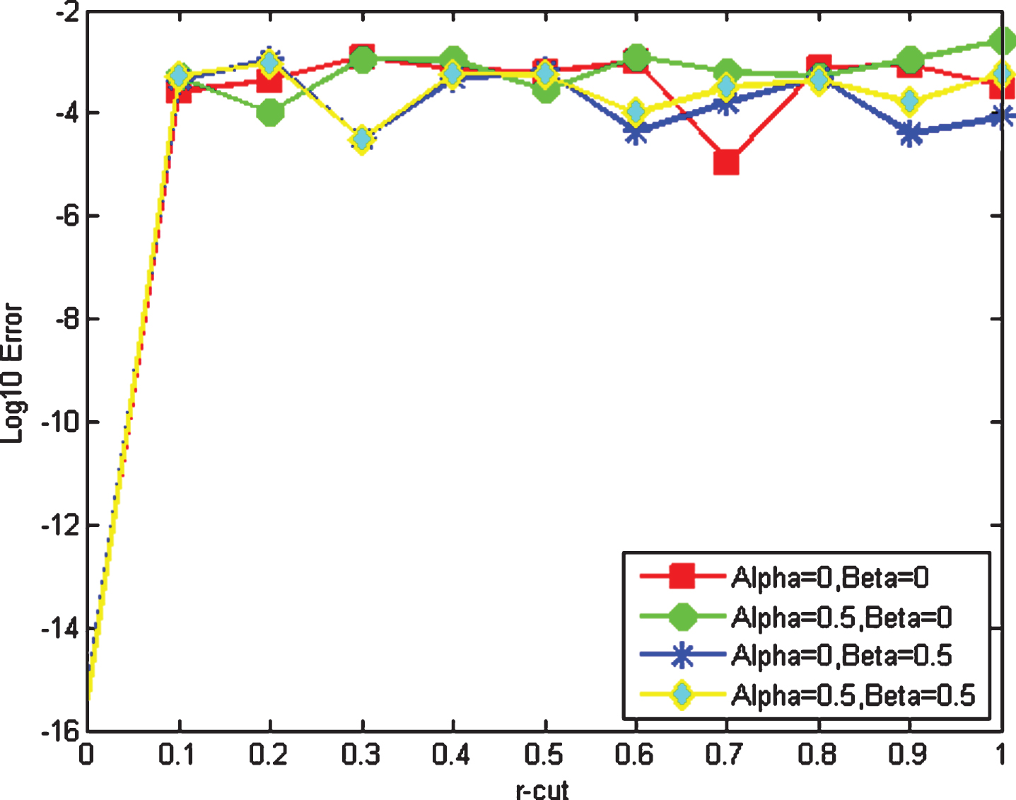
Absolute error for different value α, β of Example 1 with ν = 0.75, λ = 1.

Fig.2

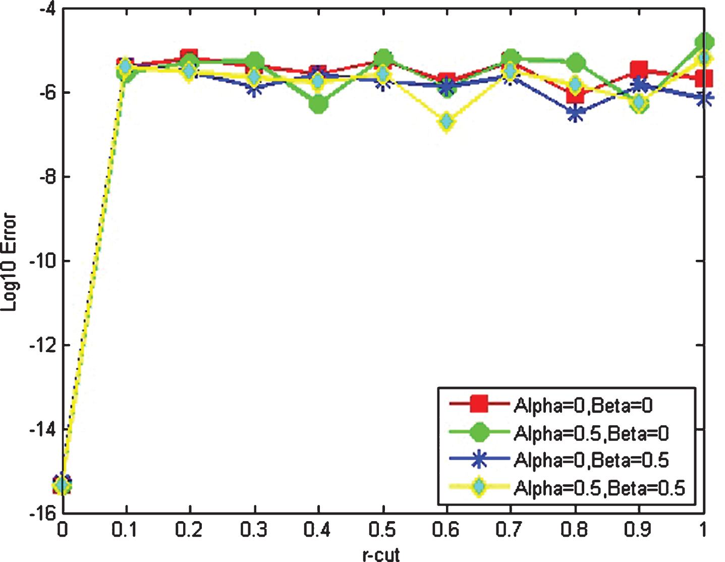
Absolute error for different value α, β of Example 1 with ν = λ = 0.75.

Examples 2. Let’s consider the inhomogeneous linear FFDE in [22, 34] ${\begin{matrix} \begin{matrix} (^{c} & D_{0^{+}}^{ν} y) (x) + y (x) = x^{4} - \frac{1}{2} x^{3} \\ - \frac{3}{Γ (4 - ν)} x^{(3 - ν)} + \frac{24}{Γ (5 - ν)} x^{(4 - ν)}, \end{matrix} \\ \begin{matrix} y^{r} (0) =, & [- 1 + r, 1 - r] 0 < r \leq 1, \\ 0 \leq x \leq 1, 0 < ν \leq 1 . \end{matrix} \end{matrix}$ (13)

Similarly, as shown in Example 1, we can gain the fuzzy approximative solution of Example 2. In Table 2, we can know that gain the good approximate solution with the high accuracy by using fractional Shifted Jacobi function. When ν = λ, the approximate solution obtained by using fractional Shifted Jacobi function is high accuracy than the one obtained by using Shifted Jacobi Polynomial. Also in Table 2, it is shown the absolute error of exact solution and approximate solution for different value of α, β. The graph of absolute error obtained by using the method proposed in [22] and this article for different value of α, β with Example 2 when m = 9 is shown in Figs. 3 and 4 respectively.

Table 2

The absolute error of JOM and SFJOM for Example 2 with different value of α, β

(α, β)	(0, 0)		(0.5, 0)		(0, 0.5)		(0.5, 0.5)
r	JOM	SFJOM	JOM	SFJOM	JOM	SFJOM	JOM	SFJOM
0.0	4.441e-16	5.551e-16	4.441e-16	4.441e-16	5.551e-16	3.331e-16	4.441e-16	4.441e-16
0.1	1.1651e-4	2.7607e-7	0.3031e-3	2.7170e-7	0.6167e-3	1.9976e-7	6.6105e-4	2.1704e-7
0.2	3.8022e-4	2.2691e-7	0.1443e-3	2.7174e-7	1.0906e-3	6.7806e-8	9.8641e-4	6.8503e-9
0.3	8.9659e-4	1.5643e-7	0.8298e-3	3.4307e-8	0.3002e-3	1.2005e-7	2.4069e-4	6.3481e-8
0.4	4.4555e-4	3.3652e-7	0.7140e-3	3.1458e-7	0.5469e-3	2.4399e-7	6.2759e-4	2.5515e-7
0.5	5.2374e-4	6.3118e-8	0.2805e-3	2.0522e-7	0.6904e-3	9.5894e-8	6.2689e-4	6.6306e-1
0.6	6.5037e-4	3.2195e-7	0.8605e-3	2.5088e-7	0.2457e-3	1.4576e-7	1.2951e-4	1.4344e-7
0.7	7.7236e-5	1.6492e-7	0.3366e-3	3.2499e-7	0.2665e-3	8.8532e-8	3.5614e-4	1.8103e-7
0.8	5.5964e-4	1.5108e-7	0.4587e-3	2.0075e-8	0.4880e-3	1.4662e-7	4.7654e-4	6.7496e-8
0.9	5.3152e-4	2.5781e-7	0.7722e-3	2.3616e-7	0.1332e-3	1.0430e-7	2.8218e-5	1.1885e-7
1.0	1.0741e-4	4.3797e-8	1.3427e-3	5.9908e-7	0.2195e-3	1.6319e-8	1.3240e-4	2.7107e-7

Fig.3

Absolute error for different value α, β of Example 2 with ν = 0.85, λ = 1.

Fig.4

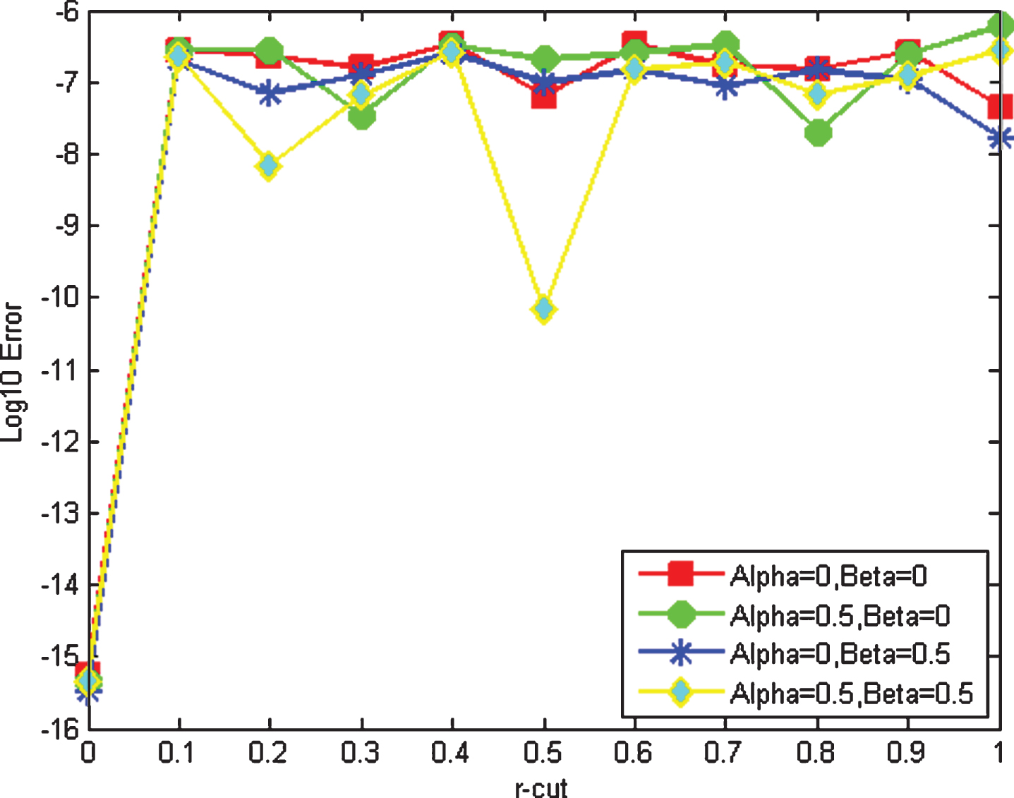
Absolute error for different value α, β of Example 2 with ν = λ = 0.85.

Example 3. Let’s consider the fuzzy fractional oscillation equation [22, 34] as ${\begin{matrix} (^{c} D_{0^{+}}^{ν} y) (x) + y (x) = {xe}^{- x}, 0 \leq x \leq 1, \\ y^{r} (0) = [- 1 + r, 1 - r], 0 < r \leq 1 . \end{matrix}$ (14)

The approximative solution of Example 3 is obtained by taking the technique proposed in Section 4.2. As above, the absolute error for some α, β when m = 7 is shown in Table 3. Figures 5 and 6 is the graph of absolute error obtained by using the method proposed in [22] and this article for different value of α, β with Example 3 when m = 7, respectively.

Table 3

The absolute error of JOM and SFJOM for Example 3 with different value of α, β

(α, β)	(0, 0)		(0.5, 0)		(0, 0.5)		(0.5, 0.5)
r	JOM	SFJOM	JOM	SFJOM	JOM	SFJOM	JOM	SFJOM
0.0	2.220e-16	3.331e-16	2.220e-16	4.441e-16	3.331e-16	4.441e-16	2.220e-16	3.331e-16
0.1	4.1474e-4	6.6859e-6	3.7026e-4	5.5052e-6	2.7533e-4	5.3015e-7	2.4195e-4	1.5889e-7
0.2	2.6574e-4	4.6936e-6	3.1592e-4	5.1173e-6	4.3337e-4	5.6251e-6	4.4575e-4	5.8499e-6
0.3	2.1485e-4	2.7739e-6	1.2463e-4	9.2943e-7	4.9498e-4	7.1033e-6	4.5134e-4	5.7567e-6
0.4	2.3441e-4	5.1363e-6	3.0800e-4	5.8578e-6	2.8083e-4	1.9442e-6	2.1916e-4	6.2265e-7
0.5	2.2236e-4	3.8593e-6	1.3812e-4	1.8179e-6	1.8225e-4	4.6771e-7	1.7721e-4	7.6168e-7
0.6	1.4570e-4	3.1531e-6	2.6929e-4	5.0515e-6	2.7219e-4	3.6345e-6	3.0425e-4	4.4781e-6
0.7	2.1845e-4	3.7251e-6	1.6009e-4	2.0846e-6	3.1066e-4	4.7220e-6	2.9205e-4	3.9755e-6
0.8	1.1692e-4	2.8661e-6	2.7766e-4	5.5474e-6	1.8416e-4	1.4090e-6	1.1572e-4	3.0285e-7
0.9	1.0597e-4	2.0266e-6	2.9153e-5	8.7866e-7	1.4294e-4	9.1008e-7	1.6474e-4	1.7621e-6
1.0	1.2029e-5	3.8970e-7	3.4411e-4	6.6518e-6	1.6270e-4	1.7026e-6	5.2326e-5	1.3266e-6

Fig.5

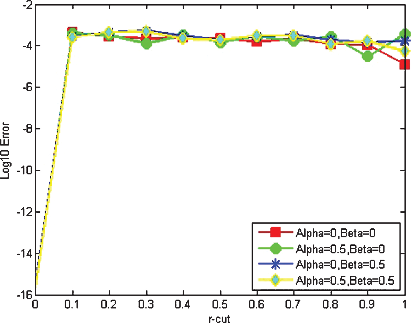
Absolute error for different value α, β of Example 3 with ν = 0.95, λ = 1.

Fig.6

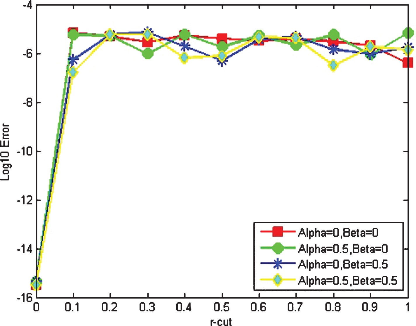
Absolute error for different value α, β of Example 3 with ν = λ = 0.95.

6 Conclusion

In this paper, we have compared the method of the fractional Jacobi operational matrix with the method of Jacobi operational matrix for solving fuzzy linear fractional differential equations. For three examples presented, the results were shown that the accuracy of numerical solutions obtained by using Jacobi operation matrix proposed in [22] are errors of about 10^-3 as shown in the Figs. 1, 3, 5 and Tables 1–3, and that the accuracy of numerical solutions obtained by using fractional Jacobi operational matrix are errors of about 10^-7 as shown in the Figs. 2, 4, 6 and Tables 1–3. For solving the fuzzy linear fractional differential equation, we have converted fuzzy differential equation into the a system of algebraic equations. And we have obtained numerical solution by using fractional Jacobi operational matrix.

The approximative solution of the above Examples 1–3 is obtained using MATLAB version R(2013A). When λ = 1, that is, in case of using Shifted Jacobi polynomials it take a little time, but when ν = λ, that is in case of fractional Jacobi functions, we can know that it take some time. Furthermore, we can understand that the absolute error changes slowly when the number of fractional Jacobi terms increase.

References

Agrawal

O.P.

, A general formulation and solution scheme for fractional optimal control problems, Nonlinear Dyn 38 (2004), 323–337.

Dehghan

, Hamedi

E.A.

and Khosravian-Arab

, A numerical scheme for the solution of a class of fractional variational and optimal control problems using the modified Jacobi polynomials, J Vib Contr 22(6) (2016), 1547–1559.

Ortigueira

M.D.

and Machado

J.A.T.

, Fractional signal processing and applications, Signal Process 83 (2003), 2285–2286.

Engheta

, On fractional calculus and fractional multipoles in electromagnetism, IEEE T Antenn Propag 44 (1996), 554–566.

Bai

, Sun

and Chen

, The existence and uniqueness of a class of fractional differential equations, Abstr Appl Anal 486040 (2014), 1–6.

L.L.

, Wang

J.R.

and Wei

, Existence and uniqueness results for fractional differential equations with boundary value conditions, Opuscula Mathematica 31(4) (2011), 629–642.

Mahto

and Abbas

, Existence and uniqueness of solution of caputo fractional differential equations, AIP Conference Proceedings 1479 (2012), 896–899.

Diethelm

, Ford

N.J.

and Freed

A.D.

, A predictor-corrector approach for the numerical solution of fractional differential equations, Nonlinear Dyn 29 (2002), 3–22.

Daftardar-Gejji

and Jafari

, Adomian decomposition: A tool for solving a system of fractional differential equations, J Math Anal Appl 301 (2005), 508–518.

10.

Das

, Analytical solution of a fractional diffusion equation by variational iteration method, Comput Math Appl 57 (2009), 483–487.

11.

Jafari

and Momani

, Solving fractional diffusion and wave equations by modified homotopy perturbation method, Phys Lett A 370 (2007), 388–396.

12.

Bhrawy

A.H.

and Alofi

A.S.

, The operational matrix of fractional integration for shifted Chebyshev polynomials, Appl Math Lett 26 (2013), 25–31.

13.

Doha

E.H.

, Bhrawy

A.H.

and Ezz-Eldien

S.S.

, A Chebyshev spectral method based on operational matrix for initial and boundary value problems of fractional order, Comput Math Appl 62 (2011), 2364–2373.

14.

Chang

R.Y.

, Chen

K.C.

and Wang

M.L.

, Modified Laguerre operational matrices for fractional calculus and applications, Int J Systems Sci 16 (1985), 1163–1172.

15.

Kazem

, Abbasbandy

and Kumar

, Fractional-order Legendre functions for solving fractional-order differential equations, Appl Math Model 37 (2013), 5498–5510.

16.

Kazem

, An integral operational matrix based on Jacobi polynomials for solving fractional-order differential equations, Appl Math Model 37 (2013), 1126–1136.

17.

Doha

E.H.

, Bhrawy

A.H.

and Ezz-Eldien

S.S.

, A new Jacobi operational matrix: An application for solving fractional differential equations, Appl Math Model 36 (2012), 4931–4943.

18.

Doha

E.H.

, Bhrawy

A.H.

, Baleanu

and Ezz-Eldien

S.S.

, On shifted Jacobi spectral approximations for solving fractional differential equations, Appl Math Comput 219 (2013), 8042–8056.

19.

Bhrawy

A.H.

and Zaky

M.A.

, Shifted fractional-order Jacobi orthogonal functions: Application to a system of fractional differential equations, Appl Math Model 40 (2016), 832–845.

20.

Mazandarani

and Vahidian Kamyad

, Modified fractional Euler method for solving fuzzy fractional initial value problem, Commun Nonlinear Sci Numer Simul 18 (2013), 12–21.

21.

Salahshour

, Allahviranloo

and Abbasbandy

, Solving fuzzy fractional differential equations by fuzzy Laplace transforms, Commun Nonlinear Sci Numer Simul 17 (2012), 1372–1381.

22.

Ahmadian

, Suleiman

, Salahshour

and Baleanu

, A Jacobi operational matrix for solving fuzzy linear fractional differential equation, Advance in Difference Equations 104 (2013), 1–29.

23.

Ahmadian

, Suleiman

and Salahshour

, An operational matrix based on Legendre polynomials for solving fuzzy fractional-order differential equations, Abstr Appl Anal 29 (2013), 1–29.

24.

Anastassiou

G.A.

, Fuzzy Mathematics: Approximation Theory. Springer, Heidelberg, 2010.

25.

Kaleva

, Fuzzy differential equations, Fuzzy Sets Syst 24 (1987), 301–317.

26.

Bede

and Stefanini

, Generalized differentiability of fuzzyvalued functions, Fuzzy Sets Syst 230 (2013), 119–141.

27.

Bede

and Gal

S.G.

, Generalizations of the differentiability of fuzzy number value functions with applications to fuzzy differential equations, Fuzzy Sets Syst 151 (2005), 581–599.

28.

Chalco-Cano

and Román-Flores

, On new solutions of fuzzy differential equations, Chaos Solitons Fractals 38 (2008), 112–119.

29.

Lakshmikantham

and Mohapatra

R.N.

, Theory of Fuzzy Differential Equations and Inclusion, Taylor Francis, 2003.

30.

Friedman

, Ming

and Kandel

, Fuzzy linear systems, Fuzzy Sets Syst 96 (1998), 201–209.

31.

Salahshour

, Allahviranloo

, Abbasbandy

and Baleanu

, Existence and uniqueness results for fractional differential equations with uncertainty, Advance in Difference Equations 112 (2012), 1–12.

32.

Diethelm

, The Analysis of Fractional Differential Equations, Lecture Notes in Mathematics. Springer, Berlin, 2010.

33.

Abbasbandy

and Amirfakhrian

, Best approximation of fuzzy functions, Nonlinear Stud 14 (2007), 87–102.

34.

Ahmadian

, Salahshour

and Chan

C.S.

, Fractional differential systems: A fuzzy solution based on operational matrix of shifted chebyshev polynomials and its applications, IEEE Transactions on Fuzzy Systems 2016 (2016), 1–18.

35.

Allahviranloo

and Afshar Kermani

, Solution of a fuzzy system of linear equation, Appl Math Comput 175 (2006), 519–531.

36.

Allahviranloo

, Armand

and Gouyandeh

, Fuzzy fractional differential equations under generalized fuzzy Caputo derivative, Journal of Intelligent & Fuzzy Systems 26 (2014), 1481–1490.

37.

Prakasha

, Nietob

J.J.

, Senthilvelavand

and Sudha Priyae

, Fuzzy fractional initial value problem, Journal of Intelligent & Fuzzy Systems 28 (2015), 2691–2704.

38.

Chehlabi

and Allahviranloo

, Concreted solutions to fuzzy linear fractional differential equations, Applied Soft Computing 44 (2016), 108–116.

39.

Armand

and Allahviranloo

, Fractional relaxation-oscillation differential equations via fuzzy variational iteration method, Journal of Intelligent & Fuzzy Systems 32 (2017), 363–371.