An imperfect EPQ model for deteriorating items with promotional effort dependent demand

Abstract

In this paper, a multi-item economic production quantity (EPQ) model for deteriorating seasonal products is developed with stock and promotional effort dependent demand in an imperfect production process. The promotional efforts are advertising, delivery facilities, better services, etc. The production process produces some imperfect quality units which are instantly reworked at a cost to bring back its quality to the perfect ones. Here, the rate of production is time dependent. Unit production cost is a function of production rate including the defective ones and the deterioration rate is considered as constant. The model is formulated as a profit maximization problem with space and budget constraints in the form of an optimal control problem. The total profit function with the effect of inflation and time-value of money is expressed as a finite integral over a finite planning horizon. The problem is solved using variational calculus to determine the minimum defective rates of the production process for which the total profit is maximum. Another three models are developed considering the constraints as uncertain (fuzzy, random and rough) in nature. For fuzzy model, three types of fuzzy numbers are considered. To deal with the fuzzy constraints, fuzzy possibility measure is used. Also, stochastic and rough constraints are reduced to the approximate crisp ones following chance constrained approach and rough expectation respectively. Numerical experiments are performed to illustrate the models. Also, some sensitivity analyses are performed and presented.

Keywords

Economic production quantity imperfect production process time-dependent demand euler-lagrange function defective rate promotional effort

1 Introduction

EPQ models are well established phenomena in the literature of inventory control problems. In most of the earlier published articles, it was assumed that the manufacturer produces 100% perfect quality products which is unrealistic. To overcome this type of situation, inventory practitioners considered the production reliability parameter (say ‘r’), which can achieve a value upto 100%. Recently, researchers have developed their models with the assumption that the manufacturers are highly satisfied if the value of ‘r’ reaches a maximum level and at the same time, they never allow ‘r’ to fall below a certain level. In this paper ‘r’ is considered in a different way, ‘r’ plays a role as a production reliability indicator, i.e., smaller value of ‘r’ provides better quality products.

Again, most of the earlier EPQ models are developed with infinite time horizon. However, in the present market scenarios, it is commonly observed that the items like i-Phone, i-Pad, fashionable clothes, etc., are periodically presented with new fetchers after a certain period of time. So, in reality, rapid change in product specifications motivates the customers to go for the new product. For this reason, the present model is developed with finite time horizon.

Deterioration of units is one of the most crucial factor in inventory control problems for seasonal products. Now-a-days, promotional effort (PE) plays a major role in creating a situation of high demand in the market. The promotional efforts are advertising, discount offer, delivery facilities, better services, etc. Among many factors, promotional effort policy is the more applicable issue in today’s business strategy. It is an important managerial insight to introduce a product, especially for the items newly launched in the market. This type of effort usually enhances the demand of any kind of commodities including deteriorating items. From retailer’s point of view, to reduce the number of deteriorated units, it is essential to reduce the time cycle and/or to increase the demand of the items. On the other hand, inventory is used to absorb fluctuations in demand. Generally, more stock motivates the customers to go for the product. Consequently, sufficient production with its inventory is planned in advance for the finite cycle period. Hence, for a real-life model, demand should be a function of stock and promotional effort of the business policy.

In this paper, a multi-item production inventory model for deteriorating items with imperfect production process is considered over a finite time horizon. Defective produced units are reworked at a cost to bring back their quality to the prefect ones. To increase the demand and to reduce time cycle, promotional effort of the business policy has been considered with the development of the model. Demands of the items depend on stock as well as promotional effort. Unit production cost is a function of production rate, raw material cost, labour charge, wear and tear cost and defective rate of the production process. As the economy of a country changes rigorously due to high inflation, the model is developed taking into account the inflation and time value of money. Incorporating the above mentioned realistic assumptions with space and budget constraints, the model is formulated as an optimal control problem for the maximization of total profit over the planning horizon and the optimum profit along with the optimum reliability indicator are obtained. Numerical experiments are performed to illustrate the models. The significance of some parameters on the proposed models are also pointed out.

2 Literature review

In imperfect production inventory models, reliability of the production process had been considered by the researchers in different approaches. Process reliability and quality improvement ware discussed first by Porteous [28] and Rosenblatt & Lee [29] in their production inventory models. They assumed that the perfect quality units are produced in the in-control state (i.e., beginning of the production process) and the imperfect quality products are produced in out-of-control state. Khouja and Mehrez [16] presented a classical inventory model and showed that the optimal production rate is smaller than the production rate which minimizes the unit production cost. After that, lot of EPQ /EMQ (Economic Manufactural Quantity) models are developed with the assumption of process reliability. In their considerations, production may be 100% perfect by introducing high quality machineries, which is unrealistic in most of the real life production systems. In reality manufacturers are highly satisfied if ‘r’ reaches a maximum level and they never allows ‘r’ to falls below a minimum level. Considering this phenomenon, recently some works have been presented by the young researchers. One can follow some notable research papers in this direction such as Sana, [34], Sarkar et al. [35], Kumar and Goswami [18] and Zhou et al. [52], etc.

Most of the production models have been formulated with infinite time horizon assuming that the demand of the items remains same for ever [3 , 47, etc.]. Items in the market, such as i-phone, Tab, i-pad, hi-fi equipments, etc. are highly demandable, but normally exist in the market for a finite time and obviously these types of demands depend on time. Various types of investigations have already been made by several authors for time-dependent demand [20, 35, etc.]. According to this assumption, product specifications also remain unchanged for ever. But, in reality unprecedental development of technology has lead to rapid change in product specifications [11] with new features. As a result, lifetimes of these types of products are normally finite and demands depend on time obviously. Hence the inventory models should be developed and analyzed for a finite period of time [15, 25, etc.] with time-dependent demand. Here, we mention an excellent article- “Celebrating a century of the economic order quantity model in honor of Ford Whitman Harris” for the researchers which is published by Cardenas-Barron et al. [4].

Deterioration of units is one of the most crucial factor in inventory control problems for deteriorating items. In the literature, there are several investigations for deteriorating items such as Yadav et al. [44]; Widyadana et al. [41]; Guchhait et al. [12, 14]; Chung et al. [7]; Baten and Khalid, [1]; Tiwari et al. [39], etc. During last two decades, there had been two excellent review articles on deterioration in the literature (Goyel and Giri 2001 and Bakker et al., 2012).

The promotional effort is an important management policy in any manufacturing sector. Goyal and Gunasekaran [10] developed a production-inventory model while demand of the end customers is influenced by advertising. Szmerekovsky and Zhang [37] developed a supply chain model with price and advertising sensitive demand. Xie & Wei [42] and Xie & Neyret [43] investigated another two interesting supply chain models to obtain optimal cooperative advertising strategies and equilibrium pricing of the chain. The works of Sana [34], Cardenas-Barron and Sana [3, 5] in this area are worth mentioning.

Incorporating inflation and time value of money, an EOQ model was presented first by Buzacott [2]. After that, several researchers such as Yang et al. [45], Sarkar et al. [35], Yang [46], etc. enlightened upon the EOQ model in this direction along with different types of demand functions. In recent years, Gilding [9] and Kumar & Rajput [19] gave their efforts to develop EPQ/EMQ models with inflation and time value of money.

Today’s competitive volatile business transaction is full of uncertainty. It is an well established phenomenon in the direction of inventory and/or production-inventory policy in recent years. After introduction of fuzzy set [50], it has been well developed and applied widely in different areas of science and technology including inventory control problems [12 , 25]. Recently, more particular, instuitionistic fuzzy set [51], hesitant fuzzy element [19 , 52] and linguistic term set [54] get considerable attention from the researchers in this field and decision making problems. On the other hand, rough set theory was first introduced by Pawlak [30] and has been developed by some authors such as Pawlak and Skowron [31], Li [21], etc. In recent years, rough set theory has been used by the young researchers to enhance the applicability of their model in different areas for the decision making problems [14, 23].

Variational principle is a simple technique for the analysis of optimal control problems. Very few researchers have developed the production -inventory models as optimal control problems and solved using this method [34, 35]. Moreover, in most of the above models, unit production cost is assumed to be constant. In practice, it varies with production rate, raw material cost, labour charge, wear and tear cost and reliability of the production process [17]. In this investigation, unit production cost is dependent on production rate, reliability indicator, raw material, labour charge and wear-and-tear costs.

3 Assumptions and notations for the proposed model

The following notations and assumptions are used in developing the model.

Notations: For i-th item following notations are used

q_i (t) is inventory level at time t (≥0) for the i-th item.

$\dot{q_{i}} (t)$ is derivative of q_i (t) with respect to t.

θ_i is the deterioration rate of the i-th item.

r_i is the defective rate of the production process for i-th item.

$r_{\min_{i}}$ and $r_{\max_{i}}$ are minimum and maximum values of r_i.

ξ_i is the variation constant of tool/die costs.

c_{d
_i} is the rework cost per defective item.

c_{h
_i} is the holding cost per unit for i-th item.

c_{3_i} is the set-up cost for i-th item.

s_{p
_i} is the unit selling price for i-th item.

a_{0_i} is the space required per unit for the produced items.

Assumptions:

In this imperfect production-inventory system, N items are produced and sold.

Life cycle of the items i.e., the planning horizon for the model under consideration, T is finite.

Production rate increases with time i.e., P_i (t) is the production rate at any time t for i-thitem.

Ω (r_i) is the development cost for production system at a stage with defective rate r_i and represents as (cf. Mettas, [27] andSana, [34]): $Ω (r_{i}) = Ω_{A_{i}} + Ω_{B_{i}} e^{Ω_{i} (r_{\max_{i}} - r_{i}) / (r_{i} - r_{\min_{i}})},$ where Ω_{A
_i} is the fixed cost like labor, energy etc., and is independent of r_i. Ω_{B
_i} is the cost of technology, resource and design complexity for production when $r_{i} = r_{\max_{i}}$ . Ω_i represents the difficulties in increasing reliability, which depends on the design complexity, technology and resource limitations etc.For seasonal/fashionable products, demand increases with time though their business period is limited and finite.

χ_i (t)=a_i - b_ie^-c_it is the promotional effort of the i-th item. Here, a_i, b_i and c_i are parameters.

Demand of the i-th item depends on stock label as well as promotional effort and is of the form D_i (t) = D_0iq (t) + D_1i + D_2iχ (t), D_0i, D_1i and D_2i are the parameters.

Unit production cost, c_{p
_i}, is a function of defective rate r_i and production rate P_i (t) and is of the form $c_{p_{i}} (r, t) = c_{r_{i}} + \frac{Ω (r_{i})}{P_{i} (t)} + ξ_{i} P_{i} (t) .$ where c_{r
_i} is the fixed material cost. Second term is the development cost which is equally distributed over the production P_i (t) at any time t, and the third term ξ_iP_i (t) is tool/die cost which is proportional to the production rate.

In the developing countries, inflation is predominant and interest rate depends on the inflation value. Thus δ = R - i, where R and i are the interest and inflation per unit currency respectively.

4 Mathematical formulation of the model

Here, the production system produces perfect quality as well as imperfect quality products. Imperfect units are reworked at a cost to bring back its quality to the original ones. In this production process, r_i plays the role as a defective rate of the production process. So, smaller value of r_i produces better quality product. Thus, the change of production and inventory level can be represented by the following differential equation: $\begin{matrix} \frac{{dq}_{i} (t)}{dt} & = & P_{i} - D_{i} - θ_{i} q_{i}, \\ i . e ., P_{i} & = & \dot{q_{i}} + D_{i} + θ_{i} q_{i}, \end{matrix}$ (1) $with q_{i} (0) = 0 and q_{i} (T) = 0, i = 1, . . ., N$ where D_i and P_i stand for D_i (t) and P_i (t) respectively.

As the production system produces N number of items, the relevant profit function, incorporating the inflation and time values of money during [0, T] is

$\begin{matrix} Z = \int_{0}^{T} e^{- δ t} \sum_{i = 1}^{N} [s_{p_{i}} D_{i} (t) - c_{p_{i}} (r, t) P_{i} (t) \\ - c_{d_{i}} r_{i} P_{i} (t) - c_{h_{i}} q_{i} (t) - c_{3_{i}} - χ_{i}] dt \end{matrix}$ (2)

Now we have to find the value of q_i (t)s, i=1,2,...N, which maximize the profit function Z and obviously, q_i (t)s must satisfy following two constraints $\sum_{i = 1}^{N} a_{0 i} q_{i} \leq S$ (3) $and \sum_{i = 1}^{N} c_{r_{i}} q_{i} \leq B$ (4) where S is the total space for the produced units and B is the budget for raw materials. Here, we formulate the augmented cost functional by introducing the Lagrange’s multiplier λ and μ (using Equation 2) as follows:

$\begin{matrix} Z_{C} = \int_{0}^{T} [\sum_{i = 1}^{N} e^{- δ t} [(s_{p_{i}} - c_{r_{i}} - c_{d_{i}} r_{i}) \\ (\dot{q_{i}} + D_{i} + θ_{i} q_{i}) - Ω (r_{i}) - ξ_{i} (\dot{q_{i}} + D_{i} \\ + θ_{i} q_{i})^{2} - c_{h_{i}} q_{i} - c_{3_{i}} - χ_{i}] \\ + λ [\sum_{i = 1}^{N} (a_{0 i} q_{i}) - S] + μ [\sum_{i = 1}^{N} (c_{r_{i}} q_{i}) - B]] dt \\ = \int_{0}^{T} Φ (q_{i}, \dot{q_{i}}, t) dt \end{matrix}$ (5) where

$\begin{matrix} Φ (q_{i}, \dot{q_{i}}, t) \\ = [\sum_{i = 1}^{N} e^{- δ t} [(s_{p_{i}} - c_{r_{i}} - c_{d_{i}} r_{i}) (\dot{q_{i}} + D_{i} + θ_{i} q_{i}) \\ - Ω (r_{i}) - ξ_{i} (\dot{q_{i}} + D_{i} + θ_{i} q_{i})^{2} - c_{h_{i}} q_{i} - c_{3_{i}} - χ_{i}] \\ + λ [\sum_{i = 1}^{N} (a_{0 i} q_{i}) - S] + μ [\sum_{i = 1}^{N} (c_{r_{i}} q_{i}) - B]] \end{matrix}$ (6)

Now, for the optimal value of Z_C, the necessary condition is the Euler-Lagrange equation. So, the problem is to find the optimal path of q (t) and P (t) for which Z_C is maximized.

Here, the Euler-Lagrange’s equation for the maximum value of Z is

$\frac{\partial Φ}{\partial q_{i}} - \frac{d}{dt} (\frac{\partial Φ}{\partial \dot{q_{i}}}) = 0 .$ (7)

Using (5) and (6), we have

$\ddot{q_{i}} - δ \dot{q_{i}} - (D_{0 i} + θ_{i}) (D_{0 i} + θ_{i} + δ) q_{i} = Ψ (t)$ (8) where Ψ (t) = L_0ie^-c_it + L_1ie^δt + L_2i and $\begin{matrix} L_{0 i} & = & - D_{2 i} b_{i} (D_{0 i} + θ_{i} + δ + c_{i}) \\ L_{1 i} & = & - (λ a_{0 i} + μ c_{r_{i}}) / 2 ξ_{i}, \\ L_{2 i} & = & (D_{1 i} + a_{i} D_{2 i}) (D_{0 i} + θ_{i} + δ) \\ + \frac{c_{hi} - (s_{p_{i}} - c_{r_{i}} - c_{d_{i}} r_{i}) (D_{0 i} + θ_{i} + δ)}{2 ξ_{i}} \end{matrix}$

Now, we have to solve the Equation (8) to get the expression for q_i (t) and that of P_i (t). For the solution the complementary function (CF) of the Equation (8) is

$q_{i} (t) = X_{1 i} e^{(D_{0 i} + θ_{i} + δ) t} + X_{2 i} e^{- (D_{0 i} + θ_{i}) t}$ (9) where X_1i and X_2i are the arbitrary constants. The particular integral (PI) of the Equation (8) is given by

$\frac{1}{D^{2} - δ D - (D_{0 i} + θ_{i}) (D_{0 i} + θ_{i} + δ)} [Ψ (t)]$ (10)

Here D ( $\equiv \frac{d}{dt}$ ) represents differential operator.

Hence, using the above equations we have,

$PI = M_{0 i} e^{- c_{i} t} + M_{1 i} e^{δ t} + M_{2 i}$ (11) where $M_{0 i} = L_{0 i} / {c_{i}^{2} + δ c_{i} - (D_{0 i} + θ_{i}) (D_{0 i} + θ_{i} + δ)}$ , M_1i = - L_1i/{(D_0i + θ_i) (D_0i + θ_i + δ)} and M_2i = - L_2i/{(D_0i + θ_i) (D_0i + θ_i + δ)}.

Hence, the complete solution of the Equation (8) is CF + PI, i.e.,

$\begin{matrix} q_{i} (t) & = & X_{1 i} e^{(D_{0 i} + θ_{i} + δ) t} + X_{2 i} e^{- (D_{0 i} + θ_{i})} \\ + M_{0 i} e^{- c_{i} t} + M_{1 i} e^{δ t} + M_{2 i} \\ = & X_{1 i} e^{K_{0 i} t} + X_{2 i} e^{K_{1 i} t} + M_{0 i} e^{- c_{i} t} \\ + M_{1 i} e^{δ t} + M_{2 i} \end{matrix}$ (12) where K_0i = (D_0i + θ_i + δ) and K_1i = - (D_0i + θ_i) Now, $\frac{{dq}_{i} (t)}{dt} = 0$ at t = t_1i (say) where the production rate is less than the demand and from the expression given below we get the value of t_1i. $K_{0 i} X_{1 i} e^{K_{0 i} t_{i}} + K_{1 i} X_{2 i} e^{K_{1 i} t_{i}} - M_{0 i} c_{i} e^{- c_{i} t_{i}} + M_{1 i} δ e^{δ t_{i}} = 0$

Again, we have q (0) =0 = q (T) and from this we get the value of X_1i and X_2i as

$\begin{matrix} X_{1 i} & = & {M_{0 i} (e^{- c_{i} T} - e^{K_{1 i} T}) + M_{1 i} (e^{δ T} - e^{K_{1 i} T}) \\ + M_{2 i} (1 - e^{K_{1 i}})} / (e^{K_{1 i} T} - e^{K_{0 i} T}) \end{matrix}$ (13) and

$\begin{matrix} X_{2 i} & = & {M_{0 i} (e^{- c_{i} T} - e^{K_{0 i} T}) + M_{1 i} (e^{δ T} - e^{K_{0 i} T}) \\ + M_{2 i} (1 - e^{K_{0 i}})} / (e^{K_{0 i} T} - e^{K_{1 i} T}) \end{matrix}$ (14)

After substituting all the values in Equation (2) we can get,

$P_{i} (t) = N_{0 i} e^{K_{0 i} t} + N_{1 i} e^{- c_{i} t} + N_{2 i} e^{δ t} + N_{3 i}$ (15) where N_0i = (K_0i - K_1i) X_1i, N_1i = - {M_0i (c_i + K_1i) + D_2ib_i}, N_2i = M_1i (δ - K_1i) and N_3i = D_1i + D_2ia_i + K_1iM_2i.

Now, putting the value of q_i (t) and that of P_i (t) (from the Equations (9) and (15) respectively) in the Equation (5), it can be evaluated the expression for $Φ (q_{i}, \dot{q_{i}}, t)$ and hence also the profit function Z_C can be obtained easily. In this problem the profit function is

$\begin{matrix} Z_{C} & = & \sum_{i = 1}^{N} [(s_{p_{i}} - c_{r_{i}} - c_{d_{i}} r_{i}) {N_{0 i} \frac{e^{(K_{0 i} - δ) t} - 1}{K_{0 i} - δ} \\ + N_{1 i} \frac{1 - e^{- (δ + c_{i}) t}}{δ + c_{i}} + N_{2 i} T + N_{3 i} \frac{1 - e^{- δ T}}{δ}} \\ - Ω (r_{i}) \frac{1 - e^{- δ T}}{δ} - ξ_{i} {N_{0 i}^{2} \frac{e^{(2 K_{0 i} - δ) T} - 1}{2 K_{0 i} - δ} \\ + N_{1 i}^{2} \frac{1 - e^{- (2 c_{i} + δ) T}}{2 c_{i} + δ} + N_{2 i}^{2} \frac{e^{δ T} - 1}{δ} + 2 N_{2 i} N_{3 i} T \\ + N_{3 i}^{2} \frac{1 - e^{- δ T}}{δ} + 2 N_{0 i} N_{1 i} \frac{e^{(K_{0 i} - c_{i} - δ) T} - 1}{K_{0 i} - c_{i} - δ} \\ + 2 N_{0 i} N_{2 i} \frac{e^{K_{0 i} T} - 1}{K_{0 i}} + 2 N_{0 i} N_{3 i} \frac{e^{(K_{0 i} - δ) T} - 1}{K_{0 i} - δ} \\ + 2 N_{1 i} N_{2 i} \frac{1 - e^{- c_{i} T}}{c_{i}} + 2 N_{1 i} N_{3 i} \frac{1 - e^{- (c_{i} + δ) T}}{c_{i} + δ}} \\ - c_{h_{i}} {X_{1 i} \frac{e^{(K_{0 i} - δ) T} - 1}{K_{0 i} - δ} + X_{2 i} \frac{e^{(K_{1 i} - δ) T} - 1}{K_{1 i} - δ} \\ + M_{0 i} \frac{1 - e^{- (c_{i} + δ) T}}{c_{i} + δ} + M_{1 i} T + M_{2 i} \frac{1 - e^{- δ T}}{δ}} \\ - {a_{i} \frac{1 - e^{- δ T}}{δ} - b_{i} \frac{1 - e^{- (c_{i} + δ) T}}{c_{i} + δ}} - c_{3_{i}} \\ \frac{(1 - e^{- δ T})}{δ} + (λ a_{0 i} + μ c_{r_{i}}) {X_{1 i} \frac{e^{(K_{0 i} T} - 1}{K_{0 i}} \\ + X_{2 i} \frac{e^{(K_{1 i} T} - 1}{K_{1 i}} + M_{0 i} \frac{1 - e^{- (c_{i} T}}{c_{i}} \\ + M_{1 i} \frac{e^{δ T} - 1}{δ} + M_{2 i} T} - (λ S + μ B) T] \end{matrix}$ (16)

Here, optimum values of λ and μ are selected by trial and error method. As this profit function contains two unknowns-r₁ and r₂, the defective rate of the production process, we again maximize Z_C with respect to r₁ and r₂ by a nol-linear gradient based method-GRG (Generalized Reduced Gradient) method using LINGO-14.

4.1 Fuzzy Model (FM)

When both the constraints are fuzzy in nature, the above problem reduces to

$\begin{matrix} Determine r_{i}, i = 1, 2, . . . N to \\ \begin{matrix} Maximize Z \\ subject to \sum_{i = 1}^{N} (a_{0 i} q_{i}) \leq \tilde{S}, \\ and \sum_{i = 1}^{N} (c_{r_{i}} q_{i}) \leq \tilde{B} \end{matrix}} \end{matrix}$ (17) where Z is given by Equation (2).

4.1.1 Triangular Fuzzy Model (TFM)

Here, $\tilde{S} = (S_{1}, S_{2}, S_{3})$ and $\tilde{B} = (B_{1}, B_{2}, B_{3})$ are fuzzy in nature and for this problem, triangular type fuzzy numbers are considered. As optimization of the objective function and constraints with fuzzy parameters are not well defined to solve the problem one can follow the following technique:

$\begin{matrix} Determine r_{i}, i = 1, 2, . . . N to \\ \begin{matrix} Maximize Z \\ s . t . pos (\sum_{i = 1}^{N} (a_{0 i} q_{i}) \leq \tilde{S}) \geq β_{1}, and \\ pos (\sum_{i = 1}^{N} (c_{r_{i}} q_{i}) \leq \tilde{B}) \geq β_{2} \end{matrix}} \end{matrix}$ (18)

Where β₁ and β₂ are predefined possibility levels that should be satisfied by the fuzzy constraints. Using the Lemma-1 (cf. Appendix), the problem reduces to

$\begin{matrix} Determine r_{i}, i = 1, 2, . . . N to \\ \begin{matrix} Maximize Z \\ subject to \\ \sum_{i = 1}^{N} (a_{0 i} q_{i}) \leq (1 - β_{1}) S_{3} + β_{1} S_{2}, \\ \sum_{i = 1}^{N} (c_{r_{i}} q_{i}) \leq (1 - β_{2}) B_{3} + β_{2} B_{2} \\ where Z is given by equation (2) . \end{matrix}} \end{matrix}$ (19)

Now, again the augmented cost functional (Z_TFN, say) can be formulate by introducing the Lagrange’s multiplier λ and μ as follows:

$\begin{matrix} Z_{TFN} \\ = \int_{0}^{T} [\sum_{i = 1}^{N} e^{- δ t} [(s_{p_{i}} - c_{r_{i}} - c_{d_{i}} r_{i}) (\dot{q_{i}} + D_{i}) \\ - Ω (r_{i}) - ξ_{i} (\dot{q_{i}} + D_{i})^{2} - c_{h_{i}} q_{i} - c_{3_{i}} - χ_{i}] \\ + λ [\sum_{i = 1}^{N} (a_{0 i} q_{i}) - {(1 - β_{1}) S_{3} + β_{1} S_{2}}] \\ + μ [\sum_{i = 1}^{N} (c_{r_{i}} q_{i}) - {(1 - β_{1}) B_{3} + β_{1} B_{2}}]] dt \\ = \int_{0}^{T} Φ_{F} (q_{i}, \dot{q_{i}}, t) dt, \end{matrix}$ (20) where

$\begin{matrix} Φ_{F} (q_{i}, \dot{q_{i}}, t) \\ = \sum_{i = 1}^{N} e^{- δ t} [(s_{p_{i}} - c_{r_{i}} - c_{d_{i}} r_{i}) (\dot{q_{i}} + D_{i}) \\ - Ω (r_{i}) - ξ_{i} (\dot{q_{i}} + D_{i})^{2} - c_{h_{i}} q_{i} - c_{3_{i}} - χ_{i}] \\ + λ [\sum_{i = 1}^{N} (a_{0 i} q_{i}) - {(1 - β_{1}) S_{3} + β_{1} S_{2}}] \\ + μ [\sum_{i = 1}^{N} (c_{r_{i}} q_{i}) - {(1 - β_{1}) B_{3} + β_{1} B_{2}}] \end{matrix}$ (21)

Proceeding as before, we get the profit function Z_TFN as follows:

$\begin{matrix} Z_{TFM} \\ = \sum_{i = 1}^{N} [(s_{p_{i}} - c_{r_{i}} - c_{d_{i}} r_{i}) {N_{0 i} \frac{e^{(K_{0 i} - δ) t} - 1}{K_{0 i} - δ} \\ + N_{1 i} \frac{1 - e^{- (δ + c_{i}) t}}{δ + c_{i}} + N_{2 i} T + N_{3 i} \frac{1 - e^{- δ T}}{δ}} \\ - Ω (r_{i}) (1 - e^{- δ T}) / δ - ξ_{i} {N_{0 i}^{2} \frac{e^{(2 K_{0 i} - δ) T} - 1}{2 K_{0 i} - δ} \\ + N_{2 i}^{2} \frac{e^{δ T} - 1}{δ} + N_{1 i}^{2} \frac{1 - e^{- (2 c_{i} + δ) T}}{2 c_{i} + δ} + 2 N_{2 i} N_{3 i} T \\ + N_{3 i}^{2} \frac{1 - e^{- δ T}}{δ} + 2 N_{0 i} N_{1 i} \frac{e^{(K_{0 i} - c_{i} - δ) T} - 1}{K_{0 i} - c_{i} - δ} \\ + 2 N_{0 i} N_{2 i} \frac{e^{K_{0 i} T} - 1}{K_{0 i}} + 2 N_{0 i} N_{3 i} \frac{e^{(K_{0 i} - δ) T} - 1}{K_{0 i} - δ} \\ + 2 N_{1 i} N_{2 i} \frac{1 - e^{- c_{i} T}}{c_{i}} + 2 N_{1 i} N_{3 i} \frac{1 - e^{- (c_{i} + δ) T}}{c_{i} + δ}} \\ - c_{h_{i}} {X_{1 i} \frac{e^{(K_{0 i} - δ) T} - 1}{K_{0 i} - δ} + X_{2 i} \frac{e^{(K_{1 i} - δ) T} - 1}{K_{1 i} - δ} \\ + M_{0 i} \frac{1 - e^{- (c_{i} + δ) T}}{c_{i} + δ} + M_{1 i} T + M_{2 i} \frac{1 - e^{- δ T}}{δ}} \\ - {a_{i} \frac{1 - e^{- δ T}}{δ} - b_{i} \frac{1 - e^{- (c_{i} + δ) T}}{c_{i} + δ}} \\ - c_{3_{i}} \frac{(1 - e^{- δ T})}{δ} + (λ a_{0 i} + μ c_{r_{i}}) \\ {X_{1 i} \frac{e^{(K_{0 i} T} - 1}{K_{0 i}} + X_{2 i} \frac{e^{(K_{1 i} T} - 1}{K_{1 i}} \\ + M_{0 i} \frac{1 - e^{- (c_{i} T}}{c_{i}} + M_{1 i} \frac{e^{δ T} - 1}{δ} + M_{2 i} T} \\ - λ {(1 - β_{1}) S_{3} + β_{1} S_{2}} T \\ - μ {(1 - β_{2}) B_{3} + β_{2} B_{2}} T] \end{matrix}$ (22)

4.1.2 Linear Fuzzy Model (LFM)

Here, $\tilde{S} = (S_{1}, S_{2})$ and $\tilde{B} = (B_{1}, B_{2})$ are considered as linear type fuzzy numbers. Using the Lemma-2 (cf. Appendix), the problem (with linear fuzzy number) reduces to

$\begin{matrix} Determine r_{i}, i = 1, 2, . . . N to \\ \begin{matrix} Maximize Z \\ s . t . \sum_{i = 1}^{N} (a_{0 i} q_{i}) \leq (1 - β_{1}) S_{2} + β_{1} S_{1}, \\ \sum_{i = 1}^{N} (c_{r_{i}} q_{i}) \leq (1 - β_{2}) B_{2} + β_{2} B_{1} \\ where Z is given by equation (2) . \end{matrix}} \end{matrix}$ (23)

Proceeding as in §4.1.1, in this case, we can derive the profit function say, Z_LFM.

4.1.3 Trapezoidal Fuzzy Model (TrFM)

Here, $\tilde{S} = (S_{1}, S_{2}, S_{3}, s_{4})$ and $\tilde{B} = (B_{1}, B_{2}, B_{3}, B_{4})$ are considered as trapezoidal type fuzzy numbers. Using the Lemma-3 (cf. Appendix), the problem (with trapezoidal fuzzy number) reducesto

$\begin{matrix} Determine r_{i}, i = 1, 2, . . . N to \\ \begin{matrix} Maximize Z \\ s . t . \sum_{i = 1}^{N} (a_{0 i} q_{i}) \leq (1 - β_{1}) S_{4} + β_{1} S_{3}, \\ \sum_{i = 1}^{N} (c_{r_{i}} q_{i}) \leq (1 - β_{2}) B_{4} + β_{2} B_{3} \\ where Z is given by equation (2) . \end{matrix}} \end{matrix}$ (24)

Proceeding as before in §4.1.1, in this case also, we can derive the profit function say, Z_TrFM.

4.2 Random Model (RAM)

When both the constraints are random in nature, the above problem reduces to

$\begin{matrix} Determine r_{i}, i = 1, 2, . . . N to \\ \begin{matrix} Maximize Z \\ subject to \sum_{i = 1}^{N} (a_{0 i} q_{i}) \leq \hat{S}, \\ and \sum_{i = 1}^{N} (c_{r_{i}} q_{i}) \leq \hat{B} \\ where Z is given by equation (2) . \end{matrix}} \end{matrix}$ (25)

Here, $\hat{S}$ and $\hat{B}$ represents the random variables. Using chance constraint programming approach (Charnes and Cooper, 1959, See Appendix), the above problem reduces to

$\begin{matrix} Determine r_{i}, i = 1, 2, . . . N to \\ \begin{matrix} Maximize Z \\ subject to \sum_{i = 1}^{N} (a_{0 i} q_{i}) \leq \bar{S} - ɛ σ_{S}, \\ and \sum_{i = 1}^{N} (c_{r_{i}} q_{i}) \leq \bar{B} - ɛ σ_{B} \\ where \Pr_{S} = \frac{1}{\sqrt{2 π}} \int_{- \infty}^{ɛ_{1}} e^{- t^{2} / 2} dt and \\ \Pr_{B} = \frac{1}{\sqrt{2 π}} \int_{- \infty}^{ɛ_{2}} e^{- t^{2} / 2} dt . \\ and Z is given by equation (2) . \end{matrix}} \end{matrix}$ (26)

Here, Pr_S and Pr_B are the probabilities with which the two constraint of (25) must hold respectively. Also, $\bar{S}$ and $\bar{B}$ are means and σ_S and σ_B and standard deviations of S and B respectively.

Now, as before, the augmented cost functional (Z_RAM, say) can be formulate by introducing the Lagrange’s multiplier λ and μ as follows:

$\begin{matrix} Z_{RAM} \\ = \int_{0}^{T} [\sum_{i = 1}^{N} e^{- δ t} [(s_{p_{i}} - c_{r_{i}} - c_{d_{i}} r_{i}) \\ \times (\dot{q_{i}} + D_{i}) - Ω (r_{i}) - ξ_{i} (\dot{q_{i}} + D_{i})^{2} \\ - c_{h_{i}} q_{i} - c_{3_{i}} - χ_{i}] \\ + λ [\sum_{i = 1}^{N} (a_{0 i} q_{i}) - {\bar{S} - ɛ σ_{S}}] \\ + μ [\sum_{i = 1}^{N} (c_{r_{i}} q_{i}) - {\bar{B} - ɛ σ_{B}}]] dt \\ = \int_{0}^{T} Φ_{RAM} (q_{i}, \dot{q_{i}}, t) dt, \end{matrix}$ (27) where

$\begin{matrix} Φ_{RAM} (q_{i}, \dot{q_{i}}, t) \\ = [\sum_{i = 1}^{N} e^{- δ t} [(s_{p_{i}} - c_{r_{i}} - c_{d_{i}} r_{i}) (\dot{q_{i}} + D_{i}) - Ω (r_{i}) \\ - ξ_{i} (\dot{q_{i}} + D_{i})^{2} - c_{h_{i}} q_{i} - c_{3_{i}} - χ_{i}] \\ + λ [\sum_{i = 1}^{N} (a_{0 i} q_{i}) - {\bar{S} - ɛ σ_{S}}] \\ + μ [\sum_{i = 1}^{N} (c_{r_{i}} q_{i}) - {\bar{B} - ɛ σ_{B}}]] \end{matrix}$ (28)

Proceeding as before, the profit function Z_RAM can be evaluated.

4.3 Rough Model (ROM)

When both the constraints are rough in nature, the above problem reduces to

$\begin{matrix} Determine r_{i}, i = 1, 2, . . . N to \\ \begin{matrix} Maximize Z \\ subject to \sum_{i = 1}^{N} (a_{0 i} q_{i}) \leq \overset{ˇ}{S}, \\ and \sum_{i = 1}^{N} (c_{r_{i}} q_{i}) \leq \overset{ˇ}{B} \\ where Z is given by equation (2) . \end{matrix}} \end{matrix}$ (29)

Here, $\overset{ˇ}{S} = ([S_{1}, S_{2}] [S_{3}, S_{4}])$ and $\overset{ˇ}{B} = ([B_{1}, B_{2}] [B_{3}, B_{4}])$ represents the rough variables. To deal with the rough variable we use rough expectation (Lemma-4) and the problem reduces to

$\begin{matrix} Determine r_{i}, i = 1, 2, . . . N to \\ \begin{matrix} Maximize Z \\ s . t . \sum_{i = 1}^{N} (a_{0 i} q_{i}) \leq \frac{1}{4} \sum_{j = 1}^{4} S_{j}, \\ \sum_{i = 1}^{N} (c_{r_{i}} q_{i}) \leq \frac{1}{4} \sum_{j = 1}^{4} B_{j}, \\ and Z is given by equation (2) . \end{matrix}} \end{matrix}$ (30)

Now, Z_ROM, the functional of this model can be represented by the following equation

$\begin{matrix} Z_{ROM} \\ = \int_{0}^{T} [\sum_{i = 1}^{N} e^{- δ t} [(s_{p_{i}} - c_{r_{i}} - c_{d_{i}} r_{i}) (\dot{q_{i}} + D_{i}) \\ - Ω (r_{i}) - ξ_{i} ({\dot{q}}_{i} + D_{i})^{2} - c_{h_{i}} q_{i} - c_{3_{i}} - χ_{i}] \\ + λ [\sum_{i = 1}^{N} (a_{0 i} q_{i}) - \frac{1}{4} \sum_{j = 1}^{4} S_{j}] \\ + μ [\sum_{i = 1}^{N} (c_{r_{i}} q_{i}) - \frac{1}{4} \sum_{j = 1}^{4} B_{j},]] dt \\ = \int_{0}^{T} Φ_{ROM} (q_{i}, \dot{q_{i}}, t) dt \end{matrix}$ (31)

where

$\begin{matrix} Φ_{ROM} (q_{i}, \dot{q_{i}}, t) \\ = [\sum_{i = 1}^{N} e^{- δ t} \\ + λ [\sum_{i = 1}^{N} (a_{0 i} q_{i}) - \frac{1}{4} \sum_{j = 1}^{4} S_{j}] \\ + μ [\sum_{i = 1}^{N} (c_{r_{i}} q_{i}) - \frac{1}{4} \sum_{j = 1}^{4} B_{j}]] \end{matrix}$ (32)

Proceeding as before, we can get the profit function Z_ROM easily.

Now, all the models are solved using a gradient based optimization technique – Generalized Reduced Gradient (GRG) method (Rao, [32]) using LINGO-12 software.

5 Numerical experiment

The models are illustrated with two items (i.e., N = 2). The parametric values used to illustrate the crisp model are presented in Table 1.

Table 1
Parametric values for crisp model

Item (i) a _i b _i c _i D _0i D _1i D _2i ξ _i c _{r
_i} c _{d
_i} c _hi Ω _i Ω _{A
_i} Ω _{B
_i} a _0i c _{3_i} s _{p
_i}

1 50 0.8 2 0.7 10 2.3 0.010 10 5 2.0 20 21 15 0.5 50 60

2 40 0.7 2 0.8 12 3 0.012 12 6 2.1 19 25 17 0.4 45 70

Item (i)	a _i	b _i	c _i	D _0i	D _1i	D _2i	ξ _i	c _{r _i}	c _{d _i}	c _hi	Ω _i	Ω _{A _i}	Ω _{B _i}	a _0i	c _{3_i}	s _{p _i}
1	50	0.8	2	0.7	10	2.3	0.010	10	5	2.0	20	21	15	0.5	50	60
2	40	0.7	2	0.8	12	3	0.012	12	6	2.1	19	25	17	0.4	45	70

Other parametric values such as B = 7850$, S = 500 units, $r_{\max_{1}} = 0.90$ , $r_{\min_{1}} = 0.2$ , $r_{\max_{2}} = 0.92$ , $r_{\min_{2}} = 0.2$ , T = 2 and δ = 0.01 are used to illustrate the crisp model. Now, with this set of parametric values, the optimum results are obtained and presented in Table 2.

Table 2

Optimum results for crisp model

λ	μ	r ₁	r ₂	B	S	Profit
2.55	0.75	0.2735	0.2801	7878.40	496.51	15679.29
2.50	0.80	0.2744	0.2835	7872.62	496.03	15684.50
2.45	0.85	0.2751	0.2831	7864.13	495.78	15687.70
2.40	0.90	0.2763	0.2819	7858.97	495.29	15692.07
2.35	0.95	0.2731	0.2851	7857.71	495.63	15694.16
2.30	1.00	0.2734	0.2833	7856.82	495.72	15695.53
2.25	1.05	0.2753	0.2842	7854.34	495.87	15696.01
2.20	1.10	0.2729	0.2812	7851.72	495.91	15696.54
2.20	1.12	0.2744	0.2831	7849.83	495.98	15697.71
2.15	1.12	0.2732	0.2857	7849.52	495.41	15696.04
2.15	1.15	0.2725	0.2846	7849.31	495.62	15694.88
2.10	1.15	0.2715	0.2859	7849.22	496.03	15693.23
2.10	1.20	0.2548	0.2745	7849.51	496.11	15692.41

Today’s competitive volatile market situation is full of uncertainties. Keeping this in mind, three sub models are developed with three different types of uncertain parameters and these are fuzzy, random and rough. In these models, it considered that both the constraints are uncertain in nature.

5.1 Optimum results of FM models

For the TFM, $\tilde{B} = (7840, 7849, 7855)$ & $\tilde{S} = (490, 501, 505)$ , for the LFM, $\tilde{B} = (7850, 7854)$ & $\tilde{S} = (498, 505)$ and for the TrFM, $\tilde{B} = (7838, 7845, 7850, 7855)$ & $\tilde{S} = (488, 494, 502, 506)$ are considered as input data. Also, T = 2 and δ = 0.01 are used to illustrate the models. The possibility label of the constraints are taken as β₁ = 0.6 and β₂ = 0.7 respectively. From the Table 2, it is found that the profit is maximum for λ = 2.20 and μ = 1.12. With these values of λ and μ (other parametric values mentioned above), the optimum results of the fuzzy models are obtained and presented in Table 3.

Table 3
Optimum results for the imprecise models

Model r ₁ r ₂ Profit Model r ₁ r ₂ Profit

TFM 0.2865 0.2901 15689.35 RAM 0.2819 0.2792 15681.28

LFM 0.2813 0.2876 15690.74 ROM 0.2888 0.2907 15687.73

TrFM 0.2835 0.2855 15689.06

Model	r ₁	r ₂	Profit	Model	r ₁	r ₂	Profit
TFM	0.2865	0.2901	15689.35	RAM	0.2819	0.2792	15681.28
LFM	0.2813	0.2876	15690.74	ROM	0.2888	0.2907	15687.73
TrFM	0.2835	0.2855	15689.06

5.2 Optimum results of RAM model

For this model, it is considered that the random variable follow normal distribution, i.e., mean of the random variables S and B are taken as $\bar{S} = 510$ and $\bar{B} = 7855$ respectively and standard deviation of the variables are taken as σ_S = 20.10 and σ_B = 30.00 respectively. For both the stochastic constraints, degree of probability Pr_S and Pr_B are taken as 0.95, i.e., ɛ = 1.645. For this input parametric values (other parametric values are same as in crisp model), the optimum results of the RAM are obtained and presented in Table 3.

5.3 Optimum results of ROM model

To illustrate the model numerically, the rough variables are taken as $\overset{ˇ}{S} = ([S_{1}, S_{2}] [S_{3}, S_{4}]) = ([497, 501] [495, 505])$ , $\overset{ˇ}{B} = ([B_{1}, B_{2}] [B_{3}, B_{4}]) = ([7848, 7851] [7840, 7855])$ . With the parametric values mentioned above (other parametric values are same as in crisp model), the optimum results of ROM are obtained and tabulated in Table 3.

5.4 Optimum results for different values of r₁ and r₂

To analyze the model perfectly, optimum results for different values of r₁ and r₂ are obtained and presented in Table 4 (crisp model) and Tables 5a(TFM), b(LFM), c(TrFM), 6(RAM) and 7(ROM) respectively.

Table 4
Optimum results of the crisp model for different values of r₁ and r₂

r ₁ r ₂ Profit r ₁ r ₂ Profit r ₁ r ₂ Profit r ₁ r ₂ Profit

0.2 15679.87 0.20 15684.56 0.20 15682.36 0.20 15677.56

0.3 15688.33 0.30 15696.54 0.30 15684.29 0.30 15679.34

0.4 15686.86 0.40 15688.46 0.40 15685.76 0.40 15678.26

0.5 0.20 15681.34 0.50 0.30 15679.35 0.50 0.40 15677.52 0.50 0.50 15675.88

0.6 15673.87 0.60 15671.36 0.60 15669.03 0.60 15667.66

0.7 15666.84 0.70 15663.55 0.70 15661.11 0.70 15659.01

0.8 15659.12 0.80 15656.01 0.80 15653.24 0.80 15650.88

0.2 15672.77 0.20 15667.26 0.20 15662.22

0.3 15671.73 0.30 15665.88 0.30 15660.86

0.4 15670.28 0.40 15663.90 0.40 15657.99

0.5 0.60 15667.23 0.50 0.70 15659.99 0.50 0.80 15654.36

0.6 15662.35 0.60 15655.97 0.60 15650.27

0.7 15656.17 0.70 15650.89 0.70 15645.36

0.8 15647.27 0.80 15642.22 0.80 15636.95

r ₁	r ₂	Profit	r ₁	r ₂	Profit	r ₁	r ₂	Profit	r ₁	r ₂	Profit
0.2		15679.87	0.20		15684.56	0.20		15682.36	0.20		15677.56
0.3		15688.33	0.30		15696.54	0.30		15684.29	0.30		15679.34
0.4		15686.86	0.40		15688.46	0.40		15685.76	0.40		15678.26
0.5	0.20	15681.34	0.50	0.30	15679.35	0.50	0.40	15677.52	0.50	0.50	15675.88
0.6		15673.87	0.60		15671.36	0.60		15669.03	0.60		15667.66
0.7		15666.84	0.70		15663.55	0.70		15661.11	0.70		15659.01
0.8		15659.12	0.80		15656.01	0.80		15653.24	0.80		15650.88
0.2		15672.77	0.20		15667.26	0.20		15662.22
0.3		15671.73	0.30		15665.88	0.30		15660.86
0.4		15670.28	0.40		15663.90	0.40		15657.99
0.5	0.60	15667.23	0.50	0.70	15659.99	0.50	0.80	15654.36
0.6		15662.35	0.60		15655.97	0.60		15650.27
0.7		15656.17	0.70		15650.89	0.70		15645.36
0.8		15647.27	0.80		15642.22	0.80		15636.95

Table 5a

Optimum results of the TFM for different values of r₁ and r₂

r ₁	r ₂	Profit	r ₁	r ₂	Profit	r ₁	r ₂	Profit	r ₁	r ₂	Profit
0.2		15678.67	0.20		15681.12	0.20		15680.45	0.20		15675.46
0.3		15685.01	0.30		15687.54	0.30		15682.79	0.30		15676.34
0.4		15683.21	0.40		15684.31	0.40		15681.06	0.40		15675.11
0.5	0.20	15677.66	0.50	0.30	15676.51	0.50	0.40	15673.88	0.50	0.50	15670.15
0.6		15671.26	0.60		15669.02	0.60		15665.83	0.60		15662.22
0.7		15664.01	0.70		15660.61	0.70		15658.11	0.70		15653.31
0.8		15656.13	0.80		15653.23	0.80		15650.23	0.80		15644.88
0.2		15672.11	0.20		15668.23	0.20		15664.22
0.3		15670.98	0.30		15667.33	0.30		15662.41
0.4		15669.28	0.40		15664.29	0.40		15658.99
0.5	0.60	15665.82	0.50	0.70	15660.24	0.50	0.80	15653.36
0.6		15658.54	0.60		15653.17	0.60		15645.16
0.7		15650.01	0.70		15643.89	0.70		15636.42
0.8		15639.44	0.80		15632.22	0.80		15624.17

Table 5b

Optimum results of the LFM for different values of r₁ and r₂

r ₁	r ₂	Profit	r ₁	r ₂	Profit	r ₁	r ₂	Profit	r ₁	r ₂	Profit
0.2		15676.12	0.20		15678.89	0.20		15677.35	0.20		15674.26
0.3		15686.21	0.30		15688.55	0.30		15683.12	0.30		15675.37
0.4		15682.83	0.40		15683.15	0.40		15680.31	0.40		15674.32
0.5	0.20	15676.34	0.50	0.30	15673.61	0.50	0.40	15671.13	0.50	0.50	15668.26
0.6		15671.22	0.60		15667.55	0.60		15664.35	0.60		15658.31
0.7		15661.62	0.70		15658.71	0.70		15656.81	0.70		15651.23
0.8		15652.17	0.80		15650.42	0.80		15648.44	0.80		15643.11
0.2		15671.34	0.20		15669.02	0.20		15664.15
0.3		15669.13	0.30		15667.56	0.30		15663.11
0.4		15667.45	0.40		15663.98	0.40		15657.37
0.5	0.60	15665.12	0.50	0.70	15661.56	0.50	0.80	15652.74
0.6		15658.83	0.60		15652.19	0.60		15642.51
0.7		15651.86	0.70		15642.17	0.70		15632.46
0.8		15638.67	0.80		15631.72	0.80		15625.32

Table 5c

Optimum results of the TrFM for different values of r₁ and r₂

r ₁	r ₂	Profit	r ₁	r ₂	Profit	r ₁	r ₂	Profit	r ₁	r ₂	Profit
0.2		15675.68	0.20		15680.25	0.20		15679.45	0.20		15673.47
0.3		15685.82	0.30		15688.34	0.30		15682.16	0.30		15674.54
0.4		15682.78	0.40		15683.47	0.40		15680.49	0.40		15672.91
0.5	0.20	15676.89	0.50	0.30	15675.44	0.50	0.40	15672.51	0.50	0.50	15669.15
0.6		15672.13	0.60		15668.73	0.60		15665.17	0.60		15661.72
0.7		15661.34	0.70		15658.33	0.70		15656.35	0.70		15650.21
0.8		15651.25	0.80		15650.21	0.80		15648.36	0.80		15640.12
0.2		15670.261	0.20		15668.03	0.20		15663.57
0.3		15667.36	0.30		15666.62	0.30		15661.89
0.4		15662.38	0.40		15663.29	0.40		15658.31
0.5	0.60	15658.22	0.50	0.70	15658.45	0.50	0.80	15652.47
0.6		15653.86	0.60		15650.47	0.60		15643.72
0.7		15646.51	0.70		15640.31	0.70		15635.11
0.8		15638.54	0.80		15630.02	0.80		15622.41

Table 6

Optimum results of the RAM for different values of r₁ and r₂

r ₁	r ₂	Profit	r ₁	r ₂	Profit	r ₁	r ₂	Profit	r ₁	r ₂	Profit
0.2		15672.56	0.20		15675.25	0.20		15674.45	0.20		15670.46
0.3		15678.12	0.30		15680.51	0.30		15677.12	0.30		15669.93
0.4		15675.35	0.40		15679.33	0.40		15673.06	0.40		15667.11
0.5	0.20	15672.02	0.50	0.30	15675.51	0.50	0.40	15667.21	0.50	0.50	15662.15
0.6		15666.66	0.60		15667.72	0.60		15660.19	0.60		15655.22
0.7		15659.45	0.70		15658.61	0.70		15653.17	0.70		15647.21
0.8		15651.24	0.80		15649.23	0.80		15645.13	0.80		15639.49
0.2		15668.11	0.20		15664.23	0.20		15659.22
0.3		15667.56	0.30		15662.33	0.30		15656.21
0.4		15665.28	0.40		15658.29	0.40		15652.01
0.5	0.60	15659.82	0.50	0.70	15653.24	0.50	0.80	15646.36
0.6		15651.54	0.60		15646.17	0.60		15639.28
0.7		15642.01	0.70		15636.89	0.70		15629.88
0.8	15633.44	0.80	15625.17	0.80	15617.03

Table 7

Optimum results of the ROM for different values of r₁ and r₂

r ₁	r ₂	Profit	r ₁	r ₂	Profit	r ₁	r ₂	Profit	r ₁	r ₂	Profit
0.2		15677.36	0.20		15679.98	0.20		15680.01	0.20		15674.71
0.3		15683.12	0.30		15686.51	0.30		15682.02	0.30		15675.82
0.4		15681.58	0.40		15682.23	0.40		15680.11	0.40		15673.92
0.5	0.20	15676.42	0.50	0.30	15675.51	0.50	0.40	15672.41	0.50	0.50	15669.78
0.6		15670.66	0.60		15668.72	0.60		15664.33	0.60		15661.35
0.7		15663.11	0.70		15659.92	0.70		15657.32	0.70		15652.01
0.8		15655.27	0.80		15652.23	0.80		15649.62	0.80		15643.29
0.2		15670.69	0.20		15667.28	0.20		15663.22
0.3		15669.95	0.30		15666.55	0.30		15660.92
0.4		15668.26	0.40		15663.12	0.40		15657.41
0.5	0.60	15664.29	0.50	0.70	15659.16	0.50	0.80	15652.36
0.6		15657.18	0.60		15652.33	0.60		15644.16
0.7		15649.29	0.70		15642.31	0.70		15634.99
0.8		15638.44	0.80		15631.92	0.80		15622.97

5.5 Discussion

From the obtained results presented in Table 2, it is reflected that the profit is higher than the other for λ = 2.20 and μ = 1.12. With the initial value of λ & μ, the profit is less and after a certain values of λ & μ, both the constraints are satisfied and the obtained profit is more than the previous. After that, though the constraints are satisfied, the profit is less than the profit for λ = 2.20 and μ = 1.12. Initially, with the decreasing and increasing value of λ and μ respectively, budget constraints of the problem is not satisfied. It may effect on the profit function of the model. As the profit is maximum for λ = 2.20 and μ = 1.12, further investigations are derived with these set of values for λ, μ.

Obtained results for all the uncertain models are presented in Table 3. To analyze the models perfectly, results for different values of r₁ and r₂ are obtained and presented in Table 4 for crisp model. It is observed that initially, the profit increases with r₁ and r₂, but after a certain values of r₁ and r₂, the profit decreases. It is also observed that, after a certain fixed value of r₂, profit of the model reflects as a decreasing function with the increasing value of r₁. If we plot the profit (Z_C) against the defective rates (r₁ and r₂) of the items, the Fig. 1, three dimensional representation of the convex profit function is obtained.

Fig.1

Graphical representation of Crisp model.

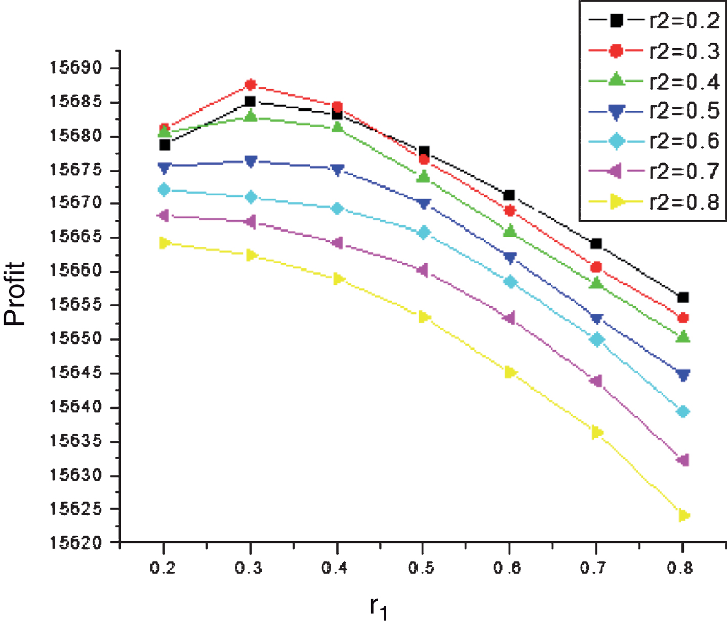
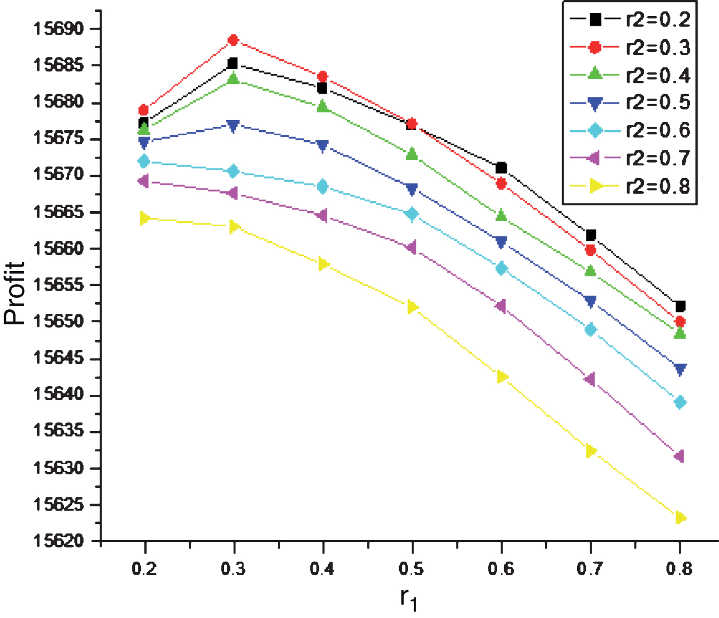
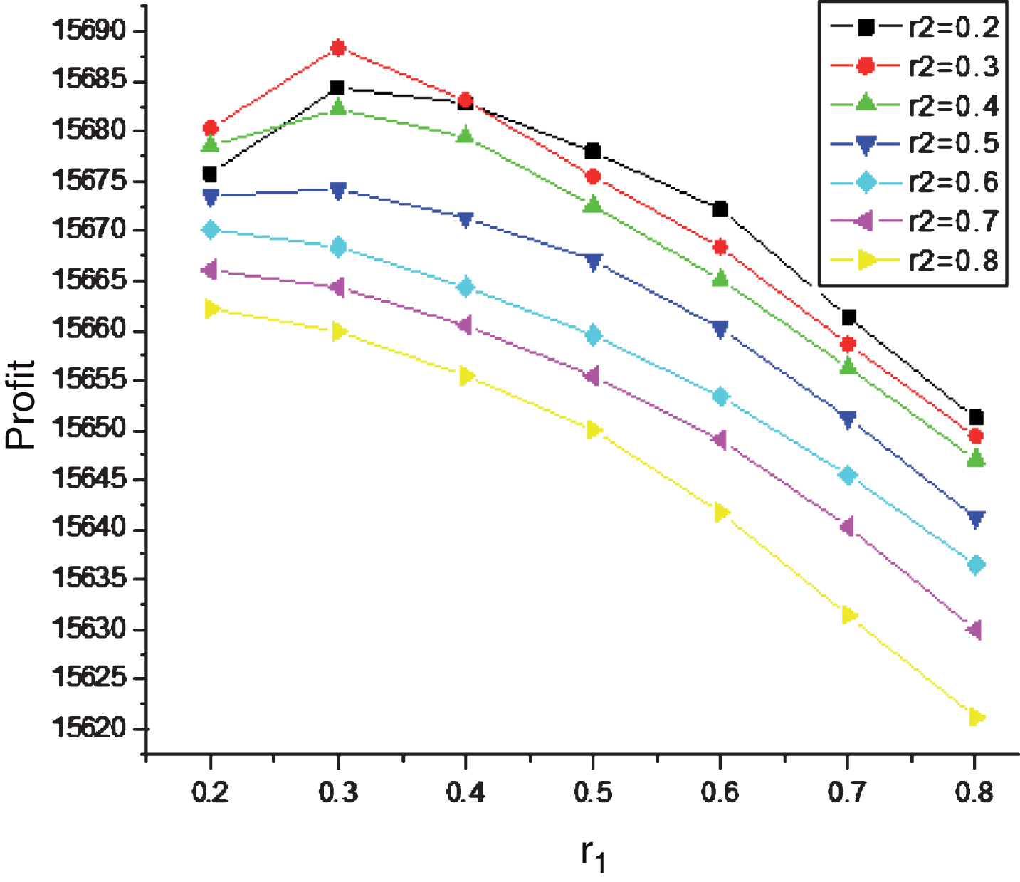
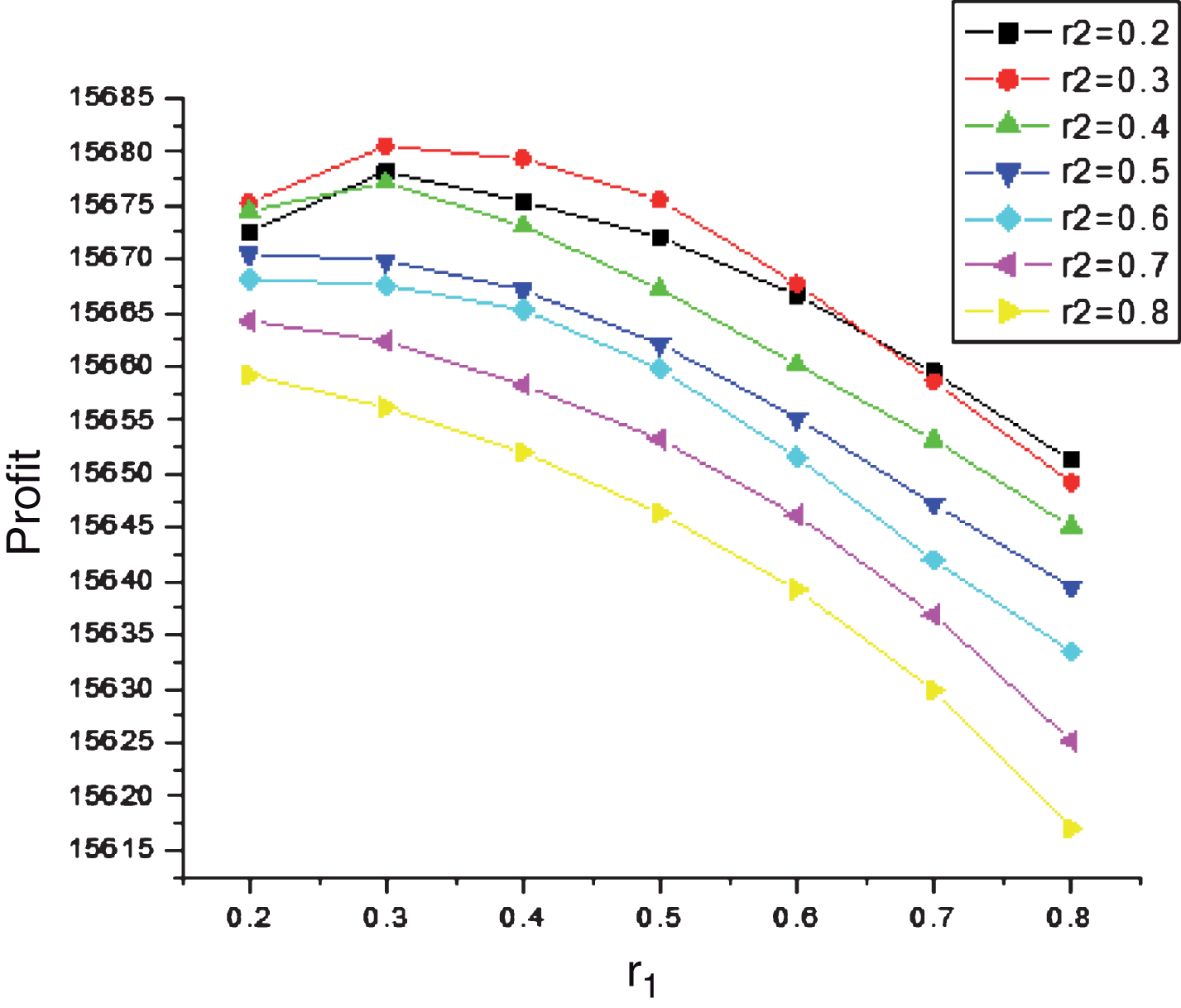
Being influenced on the crisp model, the results of the uncertain models are also obtained for different values of r₁ & r₂ and presented in Tables 5a, b, c, 6 and 7. From these tables, it is found that the nature of the profit function is similar to the crisp one. In all the cases, it is observed that initially, the profit increases with r₁ and r₂, but after the certain values of r₁ and r₂, it decreases having its convexity nature. When these are plotted graphically in a two-dimensional representation with r₁ as variable against a particular value of r₂, we obtained a maximum value (peak point) of the profit function for the crisp, fuzzy (TFM, LFM and TrFM), random and rough models which are observed from the Figs. 2–7 respectively. In all the cases, for the initial values of r₁ and r₂, profit increases but, after that these values decreases with the increase of r₁ and r₂. It is important to note that for the present models, the usual idea – the less defective rate reflects more profit is violated for some values of defective rates.

Fig.2

Profit against one defective rate for fixed values of other one.

Fig.3

Profit against one defective rate for fixed values of other one (TFM).

Fig.4

Profit against one defective rate for fixed values of other one (LFM).

Fig.5

Profit against one defective rate for fixed values of other one (TrFM).

Fig.6

Profit against one defective rate for fixed values of other one (RAM).

Fig.7

Profit against one defective rate for fixed values of other one (ROM).

Again it is observed from the Table 3 that the profit is more in LFM model and less in random model. Though it is not possible to compare the the results of uncertain models or with the crisp model, yet it can be said that the profit in crisp model is more than the uncertain models. In these uncertain models, for different profit values, many factors may play their important role. From the tables, i.e., Tables 2 and 3, it is observed that the defective rates of the production process for uncertain models, i.e., the value of r₁ and r₂ are more than that of the crisp model and the profit may be effected by the smaller value of r₁and r₂.

6 Applicability of the model

In this section, we present a real life case for ‘Singha Plastic KGP’, a company at Kharagpur railway market, India. The plastic factory produces two types of electronic plastic toys - ‘Car’ and ‘bike’. The company regularly changes its products specification to attract the children’s attention. Naturally, the time horizon for the products is finite. Here, the production process produces perfect as well as some imperfect quality products. Imperfect units are reworked at a cost to bring back its quality to the original ones. Again, quality of the items deteriorates due to several factors like bad handling, quality of the raw ingredients, etc. To increase demand, the company imposes promotional effort (PE) such as advertising, delivery facility, better service, etc. Demands (D_i) of the items depend on stock and PE of the business policy. Unit production cost (c_{p
_i}) depends on both perfect production rate and the imperfect production process. A factory has a fixed capital for business (7850$) and a godown for storage of fixed capacity (500 units).

Now, the company wants to know the optimal production reliability indicator i.e., the defective rate of the production process which determines the production rate for the whole business so that total profit of the factory is maximized.

Here, for car and bike, the set-up costs are 50$ and 45$, raw material costs 10$ and 12$, holding costs 2$ and 2.1$ per unit, rework cost 5$ and 6$ and selling prices 60$ and 70$ respectively. Time cycle for the business is 2 years.

With these set of input data, the factory management analysed the production process following the above deductions and obtained the production reliability indicators as r₁ = 0.2744 and r₂ = 0.2831 for which the optimum profit of the factory is 15697.71$.

7 Conclusion

In this article, we have studied a multi-item EPQ inventory model. The model is developed with variable production rate, demand and also defective rate of the production process together with the production rate which are controllable. In this model, promotional effort is imposed to enhance the demands of the items. Again, the present model is developed with variational principle. It is a simple technique to optimize a function appears in an integral form. To the best of our knowledge, none has studied the multi-item production inventory model using this method. In the present investigation, considering three types uncertain constraints (fuzzy, random and rough), three sub-models have been presented and solved. In fuzzy model, imprecise parameters are reduced to the crisp one following fuzzy possibility method. In random model, it is considered that the parameters follow normal distribution with known mean and standard deviation. According to the assumption, following stochastic chance constraint approach, the constraints are reduced to the equivalent crisp constraints. On the other hand, here in the rough model, parameters are transformed to the crisp constraint following rough expectation. The present investigation reveals that the defective rate of the production process is an important factor which determines the production rate and thus determines the unit production cost and optimal profit for the production-inventory managers.

This paper can be extended to two warehouse inventory model along with different types of demands such as constant demand, time-dependent demand, etc. Further research work can also be made on the optimisation problem with other environments like intuitionistic fuzzy number (IFN), hesitant fuzzy element (HFE), linguistic fuzzy number (LFN) etc.

The limitations of the present investigation are as follows:

It is fact that investigation of an optimal control problem through variational principle is easy for derivation and computation. But, if the differential equation giving the rate of change of current stock is complicated, then it is very difficult to get the Euler-Legrange equations and their solutions. To make the investigation more realistic, we have considered the crisp, fuzzy, random and rough models with finite time horizon. But, in reality, this finite time horizon may be random, fuzzy, fuzzy-randon, fuzzy-rough, IFN, LFN, etc. In future, above considerations may be taken into account by future researchers.

Footnotes

Appendix

Let $\tilde{a}$ and $\tilde{b}$ be two fuzzy numbers with membership functions $μ_{\tilde{a}} (x)$ and $μ_{\tilde{b}} (x)$ respectively. Then according to Dubois and Prade [8],

(33) $\begin{matrix} pos (\tilde{a} * \tilde{b}) & = & \sup {\min (μ_{\tilde{a}} (x), μ_{\tilde{b}} (y)), \\ x, y \in R, x * y} \end{matrix}$ where ‘pos’ represents possibility, * is any one of the relations >, < , = , ≤ , ≥ and $R$ represents set of real numbers.

(34) $nes (\tilde{a} * \tilde{b}) = 1 - pos \bar{(\tilde{a} * \tilde{b})},$ where ‘nes’ represents necessity.

Similarly possibility and necessity measures of $\tilde{a}$ with respect to $\tilde{b}$ are denoted by $Π_{\tilde{b}} (\tilde{a})$ and $N_{\tilde{b}} (\tilde{a})$ respectively and are defined as (35) $Π_{\tilde{b}} (\tilde{a}) = \sup {\min (μ_{\tilde{a}} (x), μ_{\tilde{b}} (x)), x \in R}$ (36) $N_{\tilde{b}} (\tilde{a}) = \min {\sup (μ_{\tilde{a}} (x), 1 - μ_{\tilde{b}} (x)), x \in R}$

If $\tilde{a}$ , $\tilde{b} \subseteq R$ and $\tilde{c} = f (\tilde{a}, \tilde{b})$ , where $f : R \times R \to R$ is a binary operation, membership function $μ_{\tilde{c}}$ of $\tilde{c}$ is defined as (37) $\begin{matrix} For each z \in R, \\ μ_{\tilde{c}} (z) = \sup {\min (μ_{\tilde{a}} (x), μ_{\tilde{b}} (y)), \end{matrix}$ $x, y \in R and z = f (x, y)} .$

Triangular fuzzy number (TFN): A TFN $\tilde{a} = (a_{1}, a_{2}, a_{3})$ (cf. Fig. 8) has three parameters a₁, a₂, a₃, where a₁ < a₂ < a₃ and is characterized by the membership function $μ_{\tilde{a}} (x)$ , given by

(38) $μ_{\tilde{a}} (x) = {\begin{matrix} \frac{x - a_{1}}{a_{2} - a_{1}} for a_{1} \leq x \leq a_{2} \\ \frac{a_{3} - x}{a_{3} - a_{2}} for a_{2} \leq x \leq a_{3} \\ 0 otherwise . \end{matrix}$

Linear fuzzy number (LFN): A LFN $\tilde{a} = (a_{1}, a_{2})$ (cf. Fig. 9) has two parameters a₁, a₂, where a₁ < a₂ and is characterized by the membership function $μ_{\tilde{a}} (x)$ , given by

(39) $μ_{\tilde{a}} (x) = {\begin{matrix} 1 for x \leq a_{1} \\ \frac{x - a_{1}}{a_{2} - a_{1}} for a_{1} \leq x \leq a_{2} \\ 0 for x \geq a_{2} . \end{matrix}$

Trapezoidal Fuzzy Number (TrFN): A TrFN $\tilde{a}$ is specified by four parameters (a₁, a₂, a₃, a₄) and is defined by its continuous membership function $μ_{\tilde{a}} (x)$ as follows (cf. Fig. 10):

$μ_{\tilde{A}} (x) = {\begin{matrix} \frac{x - a_{1}}{a_{2} - a_{1}} & for a_{1} \leq x \leq a_{2} \\ 1 & for a_{2} \leq x \leq a_{3} \\ \frac{a_{4} - x}{a_{4} - a_{3}} & for a_{3} \leq x \leq a_{4} \\ 0 & otherwise \end{matrix}$

According to above definitions following lemmas can easily be derived.

Lemma 1. If $\tilde{a} = (a_{1}, a_{2}, a_{3})$ be a TFN with 0 < a₁ and b is a crisp number, $pos (\tilde{a} > b) \geq x_{i}$ iff $\frac{a_{3} - b}{a_{3} - a_{2}} \geq x_{i}$ .

Lemma 2. If $\tilde{a} = (a_{1}, a_{2})$ be a LFN with 0 < a₁ and b is a crisp number, $pos (\tilde{a} > b) \geq x_{i}$ iff $\frac{a_{2} - b}{a_{2} - a_{1}} \geq x_{i}$ .

Lemma 3. If $\tilde{a} = (a_{1}, a_{2}, a_{3}, a_{4})$ be a TrFN with 0 < a₁ and b is a crisp number, $pos (\tilde{a} > b) \geq x_{i}$ iff $\frac{a_{4} - b}{a_{4} - a_{3}} \geq x_{i}$ .

$Π_{\tilde{a}} (b) = N_{\tilde{a}} (b) = {\begin{matrix} \frac{b - a_{1}}{a_{2} - a_{1}} for a_{2} \geq b \geq a_{1} \\ \frac{a_{3} - b}{a_{3} - a_{2}} for a_{3} \geq b \geq a_{2} \\ 0 otherwise . \end{matrix}$

Stochastic Non – linear Programming (SNLP) (Charnes and Cooper, [6]; Rao, [32]): Let x = (x₁, x₂, . . . , x_n) ^T be the decision vector & y = (y₁, y₂, y₃, . . . , y_N) ^T be the vector of N random variables with known mean and standard deviation, where y₁, y₂, . . . , y_N represents N parameters of the problem, then a SNLP problem can be stated in standard form as follows:

(40) $\begin{matrix} Find x = (x_{1}, x_{2}, . . ., x_{n})^{T} \\ which minimizes / maximizes f (x, y) \\ subject to P (φ_{r} (x, y) \geq 0) \geq p_{r} \\ (r = 1, . . ., m) \end{matrix}}$ where P (φ_r (x, y) ≥0) represents probability of the event φ_r (x, y) ≥0.

According to Charnes and Cooper [6] & Rao [32], if all y_i (i = 1, 2, . . . . , N) follow independent normal distribution, the stochastic problem stated above is equivalent to following crisp non-linear programming problem.

(41) $\begin{matrix} Find x = (x_{1}, x_{2}, . . ., x_{n})^{T} \\ which minimizes / maximizes f (x, \bar{y}) \\ subject to \\ {\bar{φ}}_{r} - ɛ_{r} [\sum_{i = 1}^{N} (\frac{\partial φ_{r} (x, \bar{y})}{\partial y_{i}})^{2} σ_{y_{i}}^{2}]^{\frac{1}{2}} \geq 0 \\ (r = 1, . . ., m) \\ where ɛ_{r} is given by p_{r} = \frac{1}{\sqrt{2 π}} \int_{- \infty}^{ɛ_{r}} e^{- t^{2} / 2} dt . \end{matrix}}$

Rough expectation (Liu, [22]): Let $\overset{ˇ}{X}$ be a rough variable. The expected value of the rough variable $\overset{ˇ}{X}$ is denoted by $E (\overset{ˇ}{X})$ and defined by

(42) $\begin{matrix} E (\overset{ˇ}{X}) & = & \int_{0}^{\infty} Tr (\overset{ˇ}{X} \geq r) dr \\ - \int_{- \infty}^{0} Tr (\overset{ˇ}{X} \leq r) dr \end{matrix}$ provided that at least one of the two integrals is finite. Here, ‘Tr’ represents trust measure. When the right hand side of (42) is from ∞ to -∞, the expected value is not defined.

Lemma 4 (Mondal et al., 2012): Let $\overset{ˇ}{®} = ([p, q] [r, s])$ is a rough variable, then the expected value of $\overset{ˇ}{®}$ is given by

(43) $E (\overset{ˇ}{®}) = \frac{1}{4} (p + q + r + s) .$

References

Baten

M.A.

and Khalid

, Optimal production cycle time for inventory model with linear time dependent exponential distributed deterioration, Journal of Intelligent & Fuzzy Systems30(2) (2016), 1243–1248.

Buzacott

J.A.

, Economic order quantities with ination, Operations Research Quarterly26 (1975), 553–558.

Cardenas-Barron

L.E.

and Sana

S.S.

, Multi-item EOQ inventory model in a two-layer supply chain while demand varies with a promotional effort, Applied Mathematical Modelling39(21) (2015), 6725–6737.

Cardenas-Barron

L.E.

, Chung

K.J.

and Trevio-Garza

, Celebrating a century of the economic order quantity model in honor of Ford Whitman Harris, International Journal of Production Economics155 (2014), 1–7.

Cardenas-Barron

L.E.

and Sana

S.S.

, A production-inventory model for a two-echelon supply chain when demand is dependent on sales teams’ initiatives, International Journal of Production Economics155 (2014), 249–258.

Charnes

and Cooper

W.W.

, Chance constrained programming, Management Science6 (1959), 73–79.

Chung

K.J.

, Cardenas-Barron

L.E.

and Ting

P.S.

, An inventory model with non-instantaneous receipt and exponentially deteriorating items for an integrated three layer supply chain system under two levels of trade credit, International Journal of Production Economics155 (2014), 310–317.

Dubois

and Prade

, Fuzzy sets and system - Theory and application, Academic, New York, 1980.

Gilding

B.H.

, Ination and the optimal inventory replenishment schedule with in a finite planning horizon, European Journal of Operational Research234(3) (2014), 683–693.

10.

Goyal

S.K.

and Gunasekaran

, An integrated production-inventory-marketing model for deteriorating items, Computers & Industrial Engineering28(4) (1995), 755–762.

11.

Gurnani

, Economic analysis of inventory systems, International Journal of Production Research21 (1983), 261–277.

12.

Guchhait

, Maiti

M.K.

and Maiti

, Two storage inventory model of a deteriorating item with variable demand under partial credit period, Applied Soft Computing13 (2013), 428–448.

13.

Guchhait

, Maiti

M.K.

and Maiti

, Inventory policy of a deteriorating item with variable demand under trade credit period, Computers & Industrial Engineering76 (2014), 75–88.

14.

Guchhait

, Maiti

M.K.

and Maiti

, An EOQ model of deteriorating item in imprecise environment with dynamic deterioration and credit linked demand, Applied Mathematical Modelling39 (2015), 6553–6567.

15.

Khanra

and Chaudhuri

K.S.

, A note on an ordered-level inventory model for a deteriorating item with time-dependent quadratic demand, Computers and Operations Research30 (2003), 1901–1916.

16.

Khouja

and Mehrez

, An economic production lot size model with imperfect quality and variable production rate, Journal of the Operational Research Society45(12) (1994), 1405–1417.

17.

Khouja

, The economic production lot size model under volume exibility, Computer Oper Res22 (1995), 515–525.

18.

Kumar

R.S.

and Goswami

, A fuzzy random EPQ model for imperfect quality items with possibility and necessity constraints, Applied Soft Computing34 (2015), 838–850.

19.

Kumar

and Rajput

U.S.

, An inventory model for perishable items with time varying stock dependent demand and trade credit under ination, American Journal of Operations Research5 (2015), 435–449.

20.

Lee

C.C.

and Hsu

S.L.

, A two-warehouse production model for deteriorating inventory items with time-dependent demands, European Journal of Operational Research194(3) (2009), 700–710.

21.

T.J.

, Rough approximation operators on two universes of discourse and their fuzzy extensions, Fuzzy Sets and Systems159 (2008), 3033–3050.

22.

Liu

, Theory and Practice of Uncertain Programming, Physica-Verlag, Heidelberg, 2002.

23.

and Sun

, Probabilistic rough set over two universes and rough entropy, International Journal of Approximate Reasoning53 (2012), 608–619.

24.

Maiti

M.K.

and Maiti

, Production policy for damageable items with variable cost function in an imperfect production process via genetic algorithm, Mathematical and Computer Modelling42 (2005), 977–990.

25.

Maiti

M.K.

, A fuzzy Genetic Algorithm with varying population size to solve an inventory model with credit-linked promotional demand in an imprecise planning horizon, European Journal of Operational Research213 (2011), 96–106.

26.

Mondal

, Maity

A.K.

, Maiti

M.K.

and Maiti

, A production-repairing inventory model with fuzzy rough coefficients under ination and time value of money, Appl Math Model37 (2013), 3200–3215.

27.

Mettas

, Reliability allocation and optimization for complex systems. In: Proceedings of the Annual Reliability and Maintainability Symposium. Institute Electrical and Electronics Engineers, Piscataway, NJ, pp. 216–221.

28.

Porteous

E.L.

, Optimal lot sizing, process quality improvement and set-up cost reduction, Operation Research34 (1986), 137–144.

29.

Rosenblatt

M.J.

and Lee

H.L.

, Economic production cycles with imperfect production processes, IIE Transactions17 (1986), 48–54.

30.

Pawlak

, Rough sets, Internal Journal Information Science11(5) (1982), 341–356.

31.

Pawlak

and Skowron

, Rudiments of rough sets, Information Sciences177(1) (2007), 3–27.

32.

Rao

S.S.

, Engineering optimization, theory and practice, New age International (P) Limited, India, 2000, pp. 715–761.

33.

Ray

and Chaudhuri

K.S.

, An EOQ model with stock-dependent demand, shortages, ination and time discounting, International Journal of Production Economics53 (1997), 171–180.

34.

Sana

S.S.

, A production-inventory model in an imperfect production process, European Journal of Operational Research200 (2010), 451–464.

35.

Sarkar

, Sana

S.S.

and Chaudhuri

K.S.

, An imperfect production process for time varying demand with ination and time value of money - An EMQ model, Expert System with Applications38 (2011), 13543–13548.

36.

Shah

N.H.

and Cardenas-Barron

L.E.

, Retailers decision for ordering and credit policies for deteriorating items when a supplier offers order-linked credit period or cash discount, Applied Mathematics and Computation259 (2015), 569–578.

37.

Szmerekovsky

J.G.

and Zhang

, Pricing and two-tier advertising with one manufacturer and one retailer, European Journal of Operational Research197 (2009), 785–791.

38.

Tiwari

, Cardenas-Barron

L.E.

, Khanna

and Jaggi

C.K.

, Impact of trade credit and ination on retailer’s ordering policies for non-instantaneous deteriorating items in a two-warehouse environment, International Journal of Production Economics176 (2016), 154–169.

39.

Wang

and Xu

, Admissible orders of typical hesitant fuzzy elements and their application in ordered information fusion in multi-criteria decision making, Information Fusion29 (2016), 98–104.

40.

Widyadana

G.A.

, Cardenas-Barron

L.E.

and Wee

H.M.

, Economic order quantity model for deteriorating items and planned backorder level, Mathematical and Computer Modelling54(5-6) (2011), 1569–1575.

41.

Xie

and Wei

J.C.

, Coordinating advertising and pricing in a manufacturerretailer channel, European Journal of Operational Research197 (2009), 785–791.

42.

Xie

and Neyret

, Co-op advertising and pricing models in manufacturerretailer supply chains, Computers & Industrial Engineering56 (2009), 1375–1385.

43.

Yadav

, Pundir

and Kumari

, A fuzzy multi-item production model with reliability and exibility under limited storage capacity with deterioration via geometric programming, Int J Math Oper Res3(1) (2011), 78–98.

44.

Yang

H.L.

, Teng

J.T.

and Chern

M.S.

, An inventory model under ination for deteriorating items with stock-dependent consumption rate and partial backlogging shortages, International Journal of Production Economics123(1) (2010), 819.

45.

Yang

H.L.

, Two-warehouse partial backlogging inventory models with three parameters Weibull distribution deterioration under ination, International Journal of Production Economics138(1) (2012), 107–116.

46.

Yoo

S.H.

, Kim

and Park

M.S.

, Economic production quantity model with imperfect-quality items, two-way imperfect inspection and sales return, International Journal of Production Economics121 (2009), 255–265.

47.

, Triangular hesitant fuzzy set and its application to teaching quality evaluation, Journal of Information & Computational Science10(7) (2013), 1925–1934.

48.

, Zhang

and Huang

, Dual hesitant fuzzy aggregation operators, Technological and Economic Development of Economy22(2) (2016), 194–209.

49.

Zadeh

L.A.

, Fuzzy sets, Information and Control8 (1965), 338–356.

50.

Zhou

and He

J.-M.

, Intuitionistic fuzzy normalized weighted bonferroni mean and its application in multicriteria decision making, hindawi publishing corporation, Journal of Applied Mathematics2012 (2012), 22. Article ID 136254. doi: 10.1155/2012-136254

51.

Zhou

Y.W.

, Chen

and Wu

, EPQ models for items with imperfect quality and one-time-only discount, Applied Mathematical Modelling39 (2015), 1000–1018.

52.

Zhou

and Xu

, Optimal discrete fitting aggregation approach with hesitant fuzzy information, Knowledge-Based Systems78 (2015), 22–33.

53.

Zhou

and Xu

, Generalized asymmetric linguistic term set and its application to qualitative decision making involving risk appetites, European Journal of Operational Research254 (2016), 610–621.

An imperfect EPQ model for deteriorating items with promotional effort dependent demand

Abstract

Keywords

1 Introduction

2 Literature review

3 Assumptions and notations for the proposed model

4 Mathematical formulation of the model

Table 1 Parametric values for crisp model Item (i) a i b i c i D 0i D 1i D 2i ξ i c r i c d i c hi Ω i Ω A i Ω B i a 0i c 3 i s p i 1 50 0.8 2 0.7 10 2.3 0.010 10 5 2.0 20 21 15 0.5 50 60 2 40 0.7 2 0.8 12 3 0.012 12 6 2.1 19 25 17 0.4 45 70

Table 3 Optimum results for the imprecise models Model r 1 r 2 Profit Model r 1 r 2 Profit TFM 0.2865 0.2901 15689.35 RAM 0.2819 0.2792 15681.28 LFM 0.2813 0.2876 15690.74 ROM 0.2888 0.2907 15687.73 TrFM 0.2835 0.2855 15689.06

5.3 Optimum results of ROM model

5.4 Optimum results for different values of r1 and r2

7 Conclusion

Footnotes

Appendix

References

Table 1
Parametric values for crisp model

Item (i) a _i b _i c _i D _0i D _1i D _2i ξ _i c _{r
_i} c _{d
_i} c _hi Ω _i Ω _{A
_i} Ω _{B
_i} a _0i c _{3_i} s _{p
_i}

1 50 0.8 2 0.7 10 2.3 0.010 10 5 2.0 20 21 15 0.5 50 60

2 40 0.7 2 0.8 12 3 0.012 12 6 2.1 19 25 17 0.4 45 70

Table 3
Optimum results for the imprecise models

Model r ₁ r ₂ Profit Model r ₁ r ₂ Profit

TFM 0.2865 0.2901 15689.35 RAM 0.2819 0.2792 15681.28

LFM 0.2813 0.2876 15690.74 ROM 0.2888 0.2907 15687.73

TrFM 0.2835 0.2855 15689.06

5.4 Optimum results for different values of r₁ and r₂