A supply chain of deteriorating items with variable demand

Abstract

Here two-level supply chain model is considered for a deteriorating item where the retailer’s warehouse in the market place has a limited capacity. Therefore the retailer can rent a warehouse (RW) if needed with a higher cost compared to own warehouse (OW). This model includes one wholesaler and one retailer and our aim is to maximize the total profit. The demand rate in retailer is stock-dependent and in case of any shortages, the demand is partially backlogged. Retailer also introduces some promotional cost to boost the base demand of the item. It is established that if the wholesaler shares a part of promotional cost then channel profit as well as individual profit increase. The supply chain model is also considered for imprecise environment when different inventory parameters are fuzzy/rough in nature. In this case individual profits as well as channel profit become fuzzy/rough in nature. As optimization of fuzzy/rough objective is not well defined, following credibility/trust measure of fuzzy/rough event, an approach is proposed for comparison of fuzzy/rough objectives and a Particle Swarm Optimization (PSO) algorithm is used to find marketing decisions. Models are illustrated with numerical examples.

Keywords

Deterioration Two-warehouse model Promotional Cost Credibility/Trust measure Particle Swarm Optimization

1 Introduction

In the classical inventory model for deteriorating products, it is usually assumed that the warehouse has no limits in the capacity. However, in the real-life problem the situation is different. There are a number of factors which influence the optimum solution in different ways. Sometimes these factors may suggest retailers to buy more than their own warehouse (OW) capacity. In these situations, the retailers can benefit from a rented warehouse (RW).

Today’s globalized and competitive markets drive companies to become more efficient and cost-effective. Usually, supply chain (SC) members optimize local decisions without considering the impact of their decision on the other member’s performance and on the overall performance of SC [33]. Thus, a coordination mechanism may be necessary to motivate the members. SC members are dependent on each other and these members need to be coordinated efficiently by managing dependencies between each other. Jaber and Osman [15] considered a two-level supply chain with delay in payments and profit sharing. The ordering and advertising policies for a single-period commodity was presented by Chen [3] in a two-level supply chain. Wang [32] considered a two-level supply chain with multiple retailers and stochastic demand. Dong et al. [6] developed a model on multi-level supply chain.

Many researchers have discussed on inventory models for deteriorating items. Bhunia and Maiti [2] proposed a deterministic inventory model for deteriorating items with finite rate of replenishment. Mukhopadhyay et al. [27] developed an inventory model for a deteriorating item with a price-dependent demand rate. Yang [36] considered two-warehouse partial backlogging inventory models for deteriorating items under inflation. Chung and Huang [4] proposed a two-warehouse inventory model for deteriorating items under permissible delay in payments. Dye [7] developed a deterministic inventory model for deteriorating items with time-dependent backlogging rate. Lee and Hsu [19] proposed a two-warehouse inventory model for deteriorating items with time-dependent demand. Yu et al. [38] proposed a vendor managed inventory supply chain with deteriorating raw materials and products. Mishra [26] developed a deteriorating inventory model with controllable deterioration rate for time-dependent demand and time-varying holding cost.

The demand may be influenced by the amount of the product displayed on shelves. So many researchers have considered stock-dependent demand in their research. Gayen and Pal [10] proposed a two warehouse inventory model for deteriorating items with stock-dependent demand rate and holding cost. Das et al. [5] developed a two-warehouse production model for deteriorating inventory items with stock-dependent demand under inflation over a random planning horizon. Ghiami et al. [11] formulated an inventory model for a deteriorating item with stock-dependent demand, partial backlogging and capacity constraints. Prasad and Mukherjee [30] considered stock and time dependent demand for time varying deterioration rate with shortages for optimal inventory model. From the perspective of customer buying behavior, it is seen that besides stock of products other factors such as promotional cost through advertising, free gift coupon etc., also influence customers’ preferences and their purchasing decisions and hence market demand. Many researchers also have considered promotional effort dependent demand in their research. Wu [34] considered price and promotional effort dependent demand in supply chain. Giri and Sharma [12] discussed manufacturer’s pricing strategy in a two-level supply chain with competing retailers and advertising cost dependent demand. Pal et al. [29] have considered two-echelon supply chain with price and promotional effort sensitive non-linear demand. In this investigation, it is proposed to study the effects of stock and promotional cost jointly on demand.

For some products when a retailer is out of stock, the demand is lost which means the customer finds the item or a similar one in another store. Yang et al. [37] developed an inventory model under inflation for deteriorating items with stock-dependent consumption rate and partial backlogging shortages. Sarkar and Sarkar [31] proposed an improved inventory model with partial backlogging, time varying deterioration and stock-dependent demand.

There are several methods including meta heuristic algorithms in the literature to optimize the linear and non-linear problems. Inspired by the concerted actions of flocks of birds, shoals of fish, and swarms of insects searching for food, Kennedy and Eberhart [18] originally proposed particle swarm optimization (PSO) in the mid-1990s. Particle swarm optimization (PSO) can be considered one of the most important nature-inspired computing methods in optimization research. Among the most popular nature inspired approaches, when task is to optimize with complex data or information, PSO draws significant attention. Since its introduction a very large number of applications and new ideas have been realized in the context of PSO [9 , 24]. But till now PSO is not significantly used to solve inventory control problems [14].

Due to rapid increasing complexities of the environment it is difficult to define different inventory parameters precisely. As a result it may not be possible to define the different inventory costs as well as the constraints precisely. For example production of an item in any manufacturing organization deeply depends on efficiency, effectiveness of the system, i.e., quality of the process output, inventory turnover ratio and so many factors related to the production process, which leads to uncertainty/ impreciseness in any production process. Impreciseness can be modelled using fuzzy, stochastic and rough variables. Kao and Hsu [17] discussed the inventory problem with fuzzy demands where back-orders are permitted. Maiti and Maiti [23] developed a model as a single/multi-objective programming problem under fuzzy constraint, where purchase cost, investment amount and storehouse capacity are imprecise in nature. Xu and Yao [35] introduces discrete and continuous random rough variables.

In this study, we consider a two-level supply chain consisting of a wholesaler and a retailer in which there is a limit in the retailer’s warehouse capacity. The retailer rents another warehouse to store the units. The item has a base demand d and another portion of demand which is displayed inventory dependent. Retailer invests some promotional cost to improve the base demand of the item. Amount of promotional cost is determined by the retailer. The product is deteriorated with a constant rate. Shortages are also considered and backlogged partially. It is established that if the wholesaler shares a part of the promotional cost, then the profit of both parties increase. Model is analyzed in imprecise environment also when different inventory costs like set-up cost, holding cost and the constant of the promotional cost function are fuzzy/rough in nature. As optimization of fuzzy/rough objective is not well defined, following credibility/trust measure of fuzzy/rough event is proposed for comparison of fuzzy/rough objectives. A Particle Swarm Optimization (PSO) algorithm and GRG method (using LINGO 14.0 software) are used to find optimum marketing decisions. Models are illustrated with numerical examples and compared.

Comparison of previous research works have shown in Table 1. The new ideas incorporated in this investigation are as follows:

The joint effect of stock and promotional cost on demand is considered.

The supply chain models with above demand are formulated and solved in both fuzzy and rough environments.

PSO (cf. Pakhira et al. [28]) is appropriately used for optimum results. The results for PSO and LINGO are compared in crisp environment.

Table 1
Comparison of Previous Research Works

References No. of warehouses Deterioration Stock-dependent Demand Promotional Cost Dependent Demand Other Demand Allow Shortages

Bhunia and Maiti (1998) one yes x x yes x

Mukhopadhyay et al. (2004) one yes x x yes x

Yang (2006) two yes x x yes yes

Chung and Huang (2007) two yes x x yes x

Dye (2007) one yes x x yes yes

Gayen and Pal (2009) two yes yes x x x

Lee and Hsu (2009) two yes x x yes x

Yang et al. (2010) one yes yes x x yes

Das et al. (2012) two yes yes x x x

Yu et al. (2012) one yes x x yes x

Ghiami et al. (2013) two yes yes x x yes

Sarkar and Sarkar (2013) one yes yes x x yes

Wu (2013) one x x yes yes x

Giri and Sharma (2014) one x x yes x x

Mishra (2014) one yes x x yes yes

Prasad and Mukherjee (2014) one yes yes x yes yes

Pal et al. (2015) one x x yes yes x

Present Paper two yes yes yes x yes

References	No. of warehouses	Deterioration	Stock-dependent Demand	Promotional Cost Dependent Demand	Other Demand	Allow Shortages
Bhunia and Maiti (1998)	one	yes	x	x	yes	x
Mukhopadhyay et al. (2004)	one	yes	x	x	yes	x
Yang (2006)	two	yes	x	x	yes	yes
Chung and Huang (2007)	two	yes	x	x	yes	x
Dye (2007)	one	yes	x	x	yes	yes
Gayen and Pal (2009)	two	yes	yes	x	x	x
Lee and Hsu (2009)	two	yes	x	x	yes	x
Yang et al. (2010)	one	yes	yes	x	x	yes
Das et al. (2012)	two	yes	yes	x	x	x
Yu et al. (2012)	one	yes	x	x	yes	x
Ghiami et al. (2013)	two	yes	yes	x	x	yes
Sarkar and Sarkar (2013)	one	yes	yes	x	x	yes
Wu (2013)	one	x	x	yes	yes	x
Giri and Sharma (2014)	one	x	x	yes	x	x
Mishra (2014)	one	yes	x	x	yes	yes
Prasad and Mukherjee (2014)	one	yes	yes	x	yes	yes
Pal et al. (2015)	one	x	x	yes	yes	x
Present Paper	two	yes	yes	yes	x	yes

Rest of the paper is given as follows: In Section 2 assumptions and notations required to developed the model are presented. In Section 3, mathematical formulation of the model is done. Numerical illustration is made on Section 4, discussion is made on Section 5 and a brief conclusion is presented in Section 6. Some mathematical preliminaries are given in Appendix A.

2 Assumptions and notations

The following assumptions and notations are used in this study:

Assumptions:

It is an infinite time horizon EOQ model for retailer with constantly deteriorated items.

Lead time is zero.

Demand is stock and promotional cost dependent.

Shortages are allowed and partially backlogged.

Rate of replenishment is infinite.

Two warehouses - OW and RW are considered. Sales are performed from OW and units are transferred from RW to OW by continuous release pattern.

The promotional cost to boost demand is shared by both wholesaler and retailer.

Notation	Meaning
W	capacity of the OW.
I_o (t)/I_r (t)	inventory level at the OW/RW at time t.
S (t)	shortage level at the retailer.
I_W (t)	inventory level at the wholesaler.
$I_{W}^{i} (t)$	inventory level at the wholesaler during i-th interval of its inventory period.
α	deterioration rate at the OW.
β	deterioration rate at the RW (β > α).
γ	deterioration rate at the wholesaler.
δ	percentage of demand which is backlogged during shortage time.
A_R/A_W	replenishment fixed cost per order for the retailer/ wholesaler.
p_R/p_W	purchasing price for the retailer/ wholesaler per unit.
s_R/s_W	selling price for the retailer/ wholesaler per unit (s_W = p_R).
h_o/h_r	unit holding cost per unit of time at the OW/RW.
h _W	unit holding cost per unit of time at the wholesaler.
c _sf	unit lost sale cost.
c _sv	unit shortage cost per unit of time for backlogged demand.
t _o	time at which the inventory level at the OW reaches zero.
T_R/T_W	inventory period at the retailer/ wholesaler.
Q_R/Q_W	order quantity at the retailer/ wholesaler.
D_R/D_W	quantity of deterioration at the retailer/ wholesaler.
F	fraction of the retailer’s promotion cost shared by the wholesaler.
PrC	promotional effort cost per unit time for the item: PrC = g (ρ - 1) ²d^m; where g, m are the parameters so chosen to best fit the promotional cost and d is the base demand of the item.
D (t)	demand rate at time t, the demand is assumed to be deterministic, stock-dependent and promotional cost dependent: D (t) = cI_o (t) + dρ; where c is a parameter so chosen to best fit the demandfunction.

Decision Variables	Meaning
t _r	time at which the inventory level at the RW reaches zero.
t _s	time during which the retailer is out of stock and the demand is partially backlogged.
ρ	retailer promotional effort, ρ ≥ 1.

Symbols ˜ and ˇ are used on the top of some of the above notations to indicate fuzzy and rough variable respectively.

3 Mathematical formulation

3.1 Retailer’s inventory level (OW and RW)

Considering the model, in case of having inventory at both OW and RW, the retailer uses the inventory at the RW first following continuous release pattern (cf. Fig. 1). Let I_o (t) and I_r (t) be the inventory level at the OW and the RW respectively. At the RW the inventory is depleted by a demand which is connected to the inventory level at the OW. Therefore, the changes of inventory level at the RW between the start of the inventory period and t_r can be presented by the following differential equations:

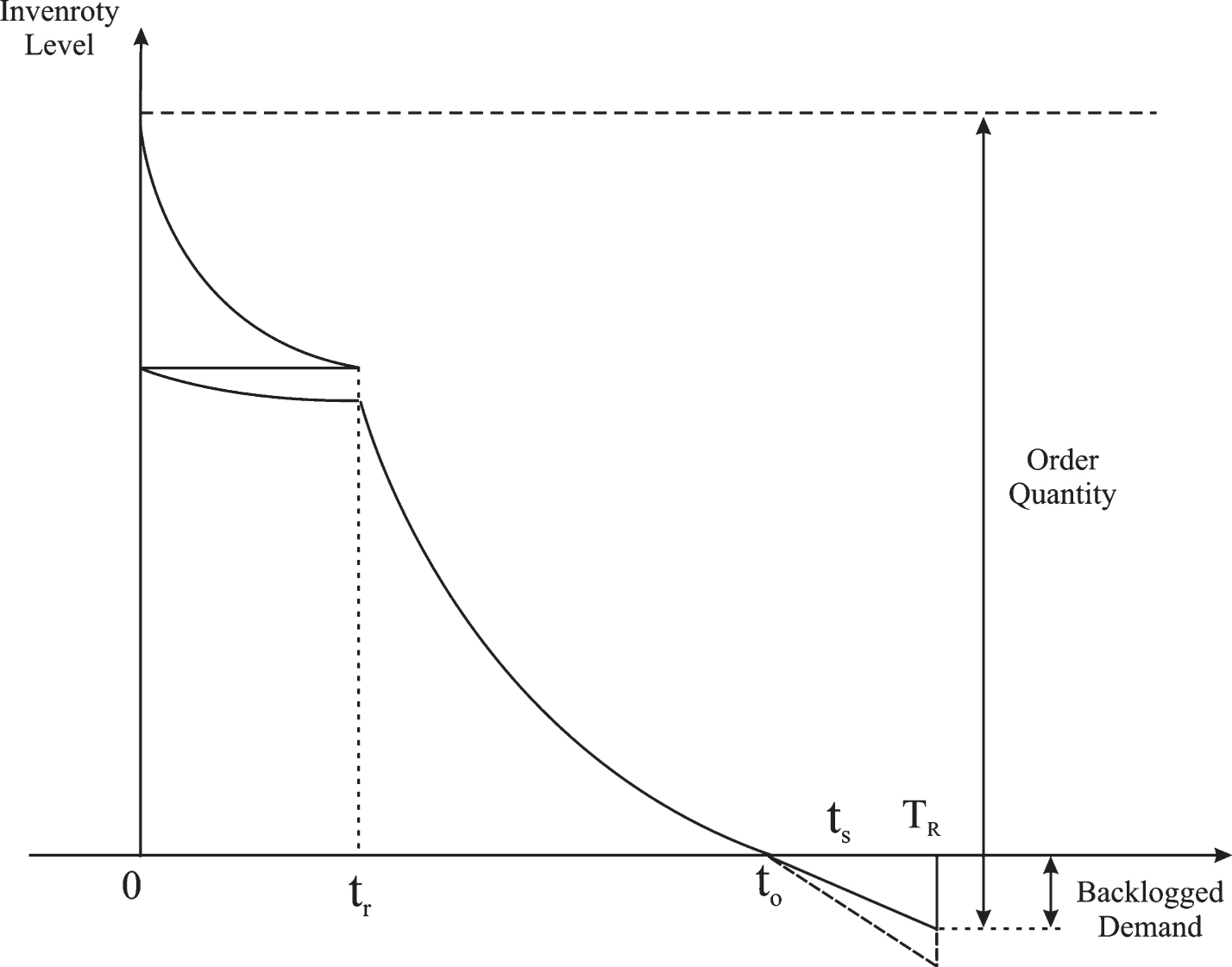
$\frac{{dI}_{r} (t)}{dt} = - c I_{o} (t) - d ρ - β I_{r} (t), for 0 \leq t \leq t_{r}$ (1)

Fig.1

Graphical presentation of the inventory level at the RW and the OW at the retailer

While the retailer is using the inventory at the RW to meet the demand, the inventory level at the OW goes down by a constant rate of the inventory level due to deterioration as follows:

$\frac{{dI}_{o} (t)}{dt} = - α I_{o} (t), for 0 \leq t \leq t_{r}$ (2)

At time t_r, the inventory at the RW is depleted completely and the inventory at the OW is used. The inventory level at the OW decreases due to the demand and deterioration until it reaches zero at t_o. This changes of inventory level at the OW is presented by the following differential equations:

$\frac{{dI}_{o} (t)}{dt} = - c I_{o} (t) - d ρ - α I_{o} (t), for t_{r} \leq t \leq t_{o}$ (3)

From t_o to T_R the system is out of stock and unmet demand is partially backlogged.

$\frac{{dI}_{o} (t)}{dt} = - δ d ρ, for t_{o} \leq t \leq T_{R}$ (4)

In order to solve the presented differential equations, the following boundary conditions should be considered: $\begin{matrix} I_{o} (0) = W, I_{o} (t_{o}) = 0, I_{r} (t_{r}) = 0 \end{matrix}$

By solving the differential equations in (1)-(4), the inventory levels at the OW and RW are obtained: $\begin{matrix} I_{r} (t) & = & \frac{{cWe}^{- α t}}{β - α} {e^{(β - α) (t_{r} - t)} - 1} \\ + \frac{d ρ}{β} {e^{β (t_{r} - t)} - 1}, for 0 \leq t \leq t_{r} \end{matrix}$ (5) $I_{o} (t) = {We}^{- α t}, for 0 \leq t \leq t_{r}$ (6) $\begin{matrix} I_{o} (t) & = & \frac{d ρ}{c + α} {e^{(c + α) (t_{o} - t)} - 1}, for t_{r} \leq t \leq t_{o} \end{matrix}$ (7) $\begin{matrix} S (t) & = & - I_{o} (t) = δ d ρ (t - t_{o}), for t_{o} \leq t \leq T_{R} \end{matrix}$ (8)

Equating the inventory level at the OW at t = t_r from (6) and (7):

$t_{o} = t_{r} + \frac{1}{c + α} \ln (1 + \frac{c + α}{d ρ} {We}^{- α t_{r}})$ (9) which shows that t_o is a function of t_r and ρ.

The order quantity for the retailer is the sum of the initial inventory level at the RW and OW and the total backlogged demand during one inventory period.

$\begin{matrix} Q_{R} & = & I_{r} (0) + I_{o} (0) + S (T_{R}) \\ = & \frac{cW}{β - α} {e^{(β - α) t_{r}} - 1} + \frac{d ρ}{β} {e^{β t_{r}} - 1} \\ + W + δ d ρ t_{s} \end{matrix}$ (10) which shows that Q_R is a function of t_r, t_s and ρ.

The length of the inventory period at the retailer is the sum of t_o and t_s.

$\begin{matrix} T_{R} = t_{o} + t_{s} \\ = t_{r} + \frac{1}{c + α} \ln (1 + \frac{c + α}{d ρ} {We}^{- α t_{r}}) + t_{s} \end{matrix}$ (11) This shows that T_R is a function of t_r, t_s and ρ.

3.2 Wholesaler’s inventory level

The order quantity and the length of the inventory period for the wholesaler are Q_W and T_W respectively. We assume that T_W is a multiplication of T_R (i.e., T_W = kT_R, where k is an integer).

The order quantity for the wholesaler is equal to the inventory needed for k periods at the retailer (i.e., kQ_R), plus the amount of deterioration during the wholesaler’s inventory cycle (i.e., D_W). It should be noted that during the k-th interval, there is no inventory in the wholesaler and, after receiving Q_W of product at the end of T_W, Q_R is sent to the retailer. Therefore there is no deterioration during this interval in the wholesaler. The order quantity for the wholesaler can be calculated as follows:

$Q_{W} = {kQ}_{R} + D_{W}$ (12) where, D_W is the deterioration during the wholesaler’s inventory cycle.

Fig. 2 illustrates the inventory level in the wholesaler. Here, one inventory period in the wholesaler consists of k retailer’s inventory periods. At the time (k - 2) T_R and (k - 1) T_R, the inventory level at the wholesaler drops by Q_R and a constant rate of the inventory is deteriorated during the interval [(k - 2) T_R, (k - 1) T_R]. The change in inventory level at the wholesaler during this interval can be presented by the following differential equation:

$\frac{{dI}_{W} (t)}{dt} = - γ I_{W} (t)$ (13)

Fig.2

Graphical presentation of the inventory level at the wholesaler

Considering the inventory level at the wholesaler at (k - 1) T_R which is Q_R, the inventory level for the specific period will be:

$\begin{matrix} I_{W} (t) & = & Q_{R} e^{γ [(k - 1) T_{R} - t]} \\ for (k - 2) T_{R} \leq t \leq (k - 1) T_{R} \end{matrix}$ (14)

In a similar way, the inventory level at the wholesaler can be obtained for the period starts at (k - 3) T_R using (13), considering the boundary condition derived from (14) at t = (k - 2) T_R:

$\begin{matrix} I_{W} (t) & = & Q_{R} (1 + e^{γ T_{R}}) e^{γ [(k - 2) T_{R} - t]} \\ for (k - 3) T_{R} \leq t \leq (k - 2) T_{R} \end{matrix}$ (15)

In this way, the inventory level at the wholesaler during i-th interval can be calculated as follow:

$\begin{matrix} I_{W}^{i} (t) & = & Q_{R} {\sum_{m = i + 1}^{k} e^{(k - m) γ T_{R}}} e^{γ [{iT}_{R} - t]} \\ for i = 1, 2, . . ., k - 1 . \end{matrix}$ (16)

3.3 Profits at the retailer

Total deterioration (D_R) during the retailer’s inventory cycle is the sum of deterioration at the RW (D_RW) and at the OW (D_OW):

$D_{R} = D_{RW} + D_{OW}$ (17) Deterioration at the RW $\begin{matrix} = D_{RW} & = & \int_{0}^{t_{r}} β I_{r} (t) dt = (e^{β t_{r}} - 1) {\frac{{cWe}^{- α t_{r}}}{β - α} + \frac{d ρ}{β}} \\ + \frac{β cW}{α (β - α)} (e^{- α t_{r}} - 1) - d ρ t_{r} \end{matrix}$ Deterioration at the OW $\begin{matrix} = D_{OW} = \int_{0}^{t_{r}} α I_{o} (t) dt + \int_{t_{r}}^{t_{o}} α I_{o} (t) dt \\ = W {1 - \frac{{ce}^{- α t_{r}}}{c + α}} - \frac{α d ρ}{c + α} (t_{o} - t_{r}) \end{matrix}$

Hence, the total selling price per unit time for the retailer:

${TS}_{R} = \frac{(Q_{R} - D_{R}) s_{R}}{T_{R}}$ (18)

The retailer has different types of cost: ordering cost (A_R), purchasing, carrying, deterioration and shortage costs. The purchasing cost for the retailer is:

${PC}_{R} = p_{R} Q_{R}$ (19)

Total inventory carrying cost (ICC_R) during the retailer’s inventory period is the sum of carrying cost at the RW (ICC_RW) and at the OW (ICC_OW):

${ICC}_{R} = {ICC}_{RW} + {ICC}_{OW}$ (20) $\begin{matrix} Carrying Cost at the RW = {ICC}_{RW} \\ = & h_{r} \int_{0}^{t_{r}} I_{r} (t) dt = \frac{h_{r}}{β} D_{RW} \\ Carrying Cost at the OW = {ICC}_{OW} \\ = & h_{o} \int_{0}^{t_{r}} I_{o} (t) dt + h_{o} \int_{t_{r}}^{t_{o}} I_{o} (t) dt = \frac{h_{o}}{α} D_{OW} \end{matrix}$

Deterioration cost (DC_R) at the retailer includes both deterioration at the RW and the OW:

${DC}_{R} = {DC}_{RW} + {DC}_{OW}$ (21) $\begin{matrix} Deterioration cost at the RW = {DC}_{RW} = p_{R} D_{RW} \\ Deterioration cost at the OW = {DC}_{OW} = p_{R} D_{OW} \end{matrix}$

During the shortage period, the demand is partially backlogged. There are two different types of shortage cost; one is based on per unit for the lost sale and the second is for backlogged demand which is per unit per unit of time.

$\begin{matrix} {SC}_{R} & = & c_{sf} \int_{t_{o}}^{T_{R}} {(1 - δ) d ρ} dt + c_{sv} \int_{t_{o}}^{T_{R}} δ d ρ (t - t_{o}) dt \\ = & c_{sf} (1 - δ) d ρ t_{s} + \frac{1}{2} c_{sv} δ d ρ t_{s}^{2} \end{matrix}$ (22)

Hence, the total cost per unit time for the retailer:

$\begin{matrix} {TC}_{R} = \frac{1}{T_{R}} (A_{R} + {PC}_{R} + {ICC}_{R} + {DC}_{R} + {SC}_{R}) \end{matrix}$ (23)

With the above costs, retailer spends some promotional cost (PrC) to increase the demand as follows:

$PrC = g (ρ - 1)^{2} d^{m}$ (24) where, g and m are the parameters so chosen to best fit the promotional cost.

Using (18), (23) and (24) the total profit per unit time of the retailer (TP_R) is:

${TP}_{R} = {TS}_{R} - {TC}_{R} - PrC$ (25)

3.4 Profits at the wholesaler

Based on (16), the amount of the deterioration in each interval can be calculated as follows:

Time Period	Deterioration
[5pt] [(k - 1) T_R, kT_R]	0
[(k - 2) T_R, (k - 1) T_R]	Q_R (e^{γT _R} - 1)
[(k - 3) T_R, (k - 2) T_R]	Q_R (e^{γT _R} - 1) (1 + e^{γT _R})
[(k - 4) T_R, (k - 3) T_R]	Q_R (e^{γT _R} - 1)
×(1 + e^{γT _R} + e^2γT_R)
…	…
[(i - 1) T_R, iT_R]	Q_R (e^{γT _R} - 1)
(i-th intervel)	$\times (\sum_{m = i + 1}^{k} e^{(k - m) γ T_{R}})$

Therefore, the total deterioration at the wholesaler (D_W) during T_W can be obtained as:

$\begin{matrix} D_{W} & = & Q_{R} (e^{γ T_{R}} - 1) \sum_{i = 1}^{k - 1} \sum_{m = i + 1}^{k} e^{(k - m) γ T_{R}} \\ = & Q_{R} (\frac{e^{k γ T_{R}} - 1}{e^{γ T_{R}} - 1} - k) \end{matrix}$ (26)

Using (12) and (26), the wholesaler’s order quantity can be calculated as follows:

$\begin{matrix} Q_{W} & = & {kQ}_{R} + Q_{R} (\frac{e^{k γ T_{R}} - 1}{e^{γ T_{R}} - 1} - k) \\ = & Q_{R} (\frac{e^{k γ T_{R}} - 1}{e^{γ T_{R}} - 1}) \end{matrix}$ (27)

Hence, the total selling price per unit time for the wholesaler:

${TS}_{W} = \frac{(Q_{W} - D_{W}) s_{W}}{T_{W}}$ (28)

The wholesaler has the following cost: ordering cost (A_W), purchasing, carrying and deterioration costs. The purchasing cost for the wholesaler is:

${PC}_{W} = p_{W} Q_{W}$ (29)

Inventory carrying cost for the wholesaler during the i-th interval is: $\begin{matrix} \int_{(i - 1) T_{R}}^{{iT}_{R}} h_{W} I_{W}^{i} (t) dt & = & \frac{h_{W} Q_{R}}{γ} (e^{γ T_{R}} - 1) \\ \times \sum_{m = i + 1}^{k} e^{(k - m) γ T_{R}} \end{matrix}$

Hence, the inventory carrying cost for the wholesaler (ICC_W) during one inventory period (consider that there is no carrying cost during k-th interval) is:

$\begin{matrix} {ICC}_{W} & = & \frac{h_{W} Q_{R}}{γ} (e^{γ T_{R}} - 1) \sum_{i = 1}^{k - 1} \sum_{m = i + 1}^{k} e^{(k - m) γ T_{R}} \\ = & \frac{h_{W} Q_{R}}{γ} (\frac{e^{k γ T_{R}} - 1}{e^{γ T_{R}} - 1} - k) = \frac{h_{W}}{γ} D_{W} \end{matrix}$ (30)

The total deterioration cost at the wholesaler (DC_W) during T_W is:

${DC}_{W} = p_{W} D_{W}$ (31)

Hence, the total cost per unit time for the wholesaler:

$\begin{matrix} {TC}_{W} = \frac{1}{T_{W}} (A_{W} + {PC}_{W} + {ICC}_{W} + {DC}_{W}) \end{matrix}$ (32)

Using (28) and (32) the total profit per unit time of the wholesaler (TP_W) is:

${TP}_{W} = {TS}_{W} - {TC}_{W}$ (33)

According to the above discussion, two cases may arise:

the wholesaler does not share any part of the promotional cost. In this case, inventory decisions are made by retailer only. i.e., only retailer’s profit is maximized to find marketing decision.

the wholesaler shares a part F of the promotional cost; i.e., the wholesaler pays Fg (ρ - 1) ²d^m and the retailer pays the remaining part (1 - F) g (ρ - 1) ²d^m of the promotional cost. In this case, inventory decisions are made by retailer and wholesaler jointly. i.e., joint profit of retailer and wholesaler is maximized to find marketing decision.

These phenomena are termed as non-coordination scenario and coordination scenario respectively. These two scenarios are discussed separately.

3.5 Non-Coordination Scenario (NCS)

In this scenario, we maximize TP_R, which is a function of t_r, t_s and ρ. So the problem is as follows:

$\begin{matrix} Determine t_{r}, t_{s}, ρ \\ to maximize {TP}_{R} (t_{r}, t_{s}, ρ) \\ subject to t_{r}, t_{s} \geq 0; ρ \geq 1 \end{matrix}}$ (34)

3.6 Coordination Scenario (CS)

In this scenario, the wholesaler offers to pay a fraction (F) of the promotional cost. Then the retailer’s profit is

$\begin{matrix} {TP}_{R}^{F} & = & {TS}_{R} - {TC}_{R} - (1 - F) g (ρ - 1)^{2} d^{m} \end{matrix}$ (35)

The wholesaler’s profit is

${TP}_{W}^{F} = {TS}_{W} - {TC}_{W} - Fg (ρ - 1)^{2} d^{m}$ (36)

Here we maximize the total profit of retailer and wholesaler (TP) and TP is a function of t_r, t_s, ρ and k.

$TP = {TP}_{R}^{F} + {TP}_{W}^{F}$ (37)

So the problem is as follows:

$\begin{matrix} \begin{matrix} Determine t_{r}, t_{s}, ρ, k \\ to maximize TP (t_{r}, t_{s}, ρ, k) \\ subject to t_{r}, t_{s} \geq 0; ρ \geq 1; k is an integer . \end{matrix}} \end{matrix}$ (38)

The retailer’s and the wholesaler’s profits under the non-coordination scenario are viewed as the lower bounds for the model under the coordination scenario. Let TP_R′ and TP_W′ be the lower bounds of retailer’s and wholesaler’s profit respectively.

true cm Proposition 1: (a) Profits for both parties increase under the coordination scenario, when the fraction of the retailer’s promotional cost is determined to be within the appropriate range (F_min, F_max), where $\begin{matrix} F_{\min} & = & [{TP}_{R^{'}} - ({TS}_{R} - {TC}_{R} - PrC)] / PrC \\ and F_{\max} & = & [({TS}_{W} - {TC}_{W}) - {TP}_{W^{'}}] / PrC \end{matrix}$ (b) When the wholesaler and the retailer have the same bargaining power, the appropriate fraction of the promotional cost sharing is F = (F_max + F_min)/2.

Proof: (a) From Retailer’s point of view for CS $\begin{matrix} (Profits in CS) - (Profits in NCS) \geq 0 \\ \Rightarrow & {TP}_{R}^{F} (t_{r}, t_{s}, ρ) - {TP}_{R^{'}} \geq 0 \\ \Rightarrow & {{TS}_{R} - {TC}_{R} - (1 - F) PrC} - {TP}_{R^{'}} \geq 0 \\ \Rightarrow & F . PrC \geq {TP}_{R^{'}} - ({TS}_{R} - {TC}_{R} - PrC) \\ \Rightarrow & F \geq [{TP}_{R^{'}} - ({TS}_{R} - {TC}_{R} - PrC)] / PrC \\ = F_{\min} (say) \end{matrix}$ Also from wholesaler’s point of view for CS $\begin{matrix} (Profits in CS) - (Profits in NCS) \geq 0 \\ \Rightarrow & {TP}_{W}^{F} (t_{r}, t_{s}, ρ, k) - {TP}_{W^{'}} \geq 0 \\ \Rightarrow & {{TS}_{W} - {TC}_{W} - F . PrC} - {TP}_{W^{'}} \geq 0 \\ \Rightarrow & F \leq [({TS}_{W} - {TC}_{W}) - {TP}_{W^{'}}] / PrC \\ = F_{\max} (say) \end{matrix}$ Hence, F_min ≤ F ≤ F_max.

(b) For the proofs of this part, readers may follow Pakhira et al. [28].

3.7 Fuzzy model

As discussed in the introduction section that in real life most of the inventory parameters are fuzzy in nature. When some of the inventory parameters are fuzzy in nature model reduces to a fuzzy model. Normally set up cost, holding cost are imprecise in nature. In this model let us consider set up costs A_R, A_W, holding costs h_r, h_o, h_W and the constant g of the promotional cost as fuzzy numbers ${\tilde{A}}_{R}$ , ${\tilde{A}}_{W}$ , ${\tilde{h}}_{r}$ , ${\tilde{h}}_{o}$ , ${\tilde{h}}_{W}$ , $\tilde{g}$ respectively, then profits in both the scenario become imprecise in nature.

3.7.1 Fuzzy model in non-coordination scenario

According to the above assumptions in this case individual profits and total profit of retailer and wholesaler are reduces to fuzzy numbers and represented by $\begin{matrix} {\tilde{TP}}_{R} & = & {TS}_{R} - {\tilde{TC}}_{R} - \tilde{PrC} \\ {\tilde{TP}}_{W} & = & {TS}_{W} - {\tilde{TC}}_{W} \\ \tilde{TP} & = & {\tilde{TP}}_{R} + {\tilde{TP}}_{W} \end{matrix}$ where, $\begin{matrix} {\tilde{TC}}_{R} & = & \frac{1}{T_{R}} ({\tilde{A}}_{R} + {PC}_{R} + {\tilde{ICC}}_{R} + {DC}_{R} + {SC}_{R}) \\ \tilde{PrC} & = & \tilde{g} (ρ - 1)^{2} d^{m} \\ {\tilde{TC}}_{W} & = & \frac{1}{T_{W}} ({\tilde{A}}_{W} + {PC}_{W} + {\tilde{ICC}}_{W} + {DC}_{W}) \end{matrix}$

$\begin{matrix} where, {\tilde{ICC}}_{R} & = & \frac{{\tilde{h}}_{r}}{β} D_{RW} + \frac{{\tilde{h}}_{o}}{α} D_{OW} \\ {\tilde{ICC}}_{W} & = & \frac{{\tilde{h}}_{W}}{γ} D_{W} \end{matrix}$

Considering the fuzzy numbers ${\tilde{A}}_{R}$ , ${\tilde{A}}_{W}$ , ${\tilde{h}}_{r}$ , ${\tilde{h}}_{o}$ , ${\tilde{h}}_{W}$ , $\tilde{g}$ as TFNs (A_R1, A_R2, A_R3), (A_W1, A_W2, A_W3), (h_r1, h_r2, h_r3), (h_o1, h_o2, h_o3), (h_W1, h_W2, h_W3), (g₁, g₂, g₃) respectively, the fuzzy numbers ${\tilde{TP}}_{R}$ , ${\tilde{TP}}_{W}$ , $\tilde{TP}$ becomes (TP_R1, TP_R2, TP_R3), (TP_W1, TP_W2, TP_W3), (TP₁, TP₂, TP₃) respectively, where

For i = 1, 2, 3 $\begin{matrix} {TP}_{Ri} & = & {TS}_{R} - {TC}_{R (4 - i)} - {PrC}_{4 - i} \\ {TP}_{Wi} & = & {TS}_{W} - {TC}_{W (4 - i)} \\ {TP}_{i} & = & {TP}_{Ri} + {TP}_{Wi} \end{matrix}$ where, $\begin{matrix} {TC}_{Ri} & = & \frac{1}{T_{R}} (A_{Ri} + {PC}_{R} + {ICC}_{Ri} + {DC}_{R} + {SC}_{R}) \\ {PrC}_{i} & = & g_{i} (ρ - 1)^{2} d^{m} \\ {TC}_{Wi} & = & \frac{1}{T_{W}} (A_{Wi} + {PC}_{W} + {ICC}_{Wi} + {DC}_{W}) \end{matrix}$ where, $\begin{matrix} {ICC}_{Ri} & = & \frac{h_{ri}}{β} D_{RW} + \frac{h_{oi}}{α} D_{OW} \\ {ICC}_{Wi} & = & \frac{h_{Wi}}{γ} D_{W} \end{matrix}$ So in this case the problem reduces to:

$\begin{matrix} Maximize {\tilde{TP}}_{R} = ({TP}_{R 1}, {TP}_{R 2}, {TP}_{R 3}) \\ subject to t_{r}, t_{s} \geq 0; ρ \geq 1 \end{matrix}}$ (39) The problem is solved using proposed PSO where comparisons of the objectives are made by the following approach. Let ${\tilde{TP}}_{Ra}$ , ${\tilde{TP}}_{Rb}$ be the two objectives corresponding to two solutions X_a, X_b respectively. Then the approach of comparison of solutions is given below:

In this approach credibility measure of fuzzy event is used to compare the solutions. According to this approach X_a dominates X_b if Cr( ${\tilde{TP}}_{Ra} > {\tilde{TP}}_{Rb}) > 0.5$ . In this approach no crisp equivalent of fuzzy numbers are used to find marketing decisions.

3.7.2 Fuzzy model in coordination scenario

For the coordination scenario the individual profits and total profit as fuzzy numbers are represented by $\begin{matrix} {\tilde{TP}}_{R}^{F} & = & {TS}_{R} - {\tilde{TC}}_{R} - (1 - F) . \tilde{PrC} \\ {\tilde{TP}}_{W}^{F} & = & {TS}_{W} - {\tilde{TC}}_{W} - F . \tilde{PrC} \\ \tilde{TP} & = & {\tilde{TP}}_{R}^{F} + {\tilde{TP}}_{W}^{F} \end{matrix}$ So in this case the problem reduces to:

$\begin{matrix} \begin{matrix} Maximize {\tilde{TP}}_{W} = ({TP}_{W 1}, {TP}_{W 2}, {TP}_{W 3}) \\ subject to t_{r}, t_{s} \geq 0; ρ \geq 1; k is an integer \end{matrix}} \end{matrix}$ (40) The problem is solved using proposed PSO where comparisons of the objectives are made by using Credibility Measure approach, which are discussed above.

3.8 Rough model

In this model let us consider set up costs A_R, A_W, holding costs h_r, h_o, h_W and the constant g of the promotional cost as rough variables ${\overset{ˇ}{A}}_{R}$ , ${\overset{ˇ}{A}}_{W}$ , ${\overset{ˇ}{h}}_{r}$ , ${\overset{ˇ}{h}}_{o}$ , ${\overset{ˇ}{h}}_{W}$ , $\overset{ˇ}{g}$ respectively, then profits in both the scenario become imprecise in nature.

3.8.1 Rough model in non-coordination scenario

According to the above assumptions in this case individual profits and total profit of retailer and wholesaler are reduces to rough variables and represented by $\begin{matrix} {\overset{ˇ}{TP}}_{R} & = & {TS}_{R} - {\overset{ˇ}{TC}}_{R} - \overset{ˇ}{PrC} \\ {\overset{ˇ}{TP}}_{W} & = & {TS}_{W} - {\overset{ˇ}{TC}}_{W} \\ \overset{ˇ}{TP} & = & {\overset{ˇ}{TP}}_{R} + {\overset{ˇ}{TP}}_{W} \end{matrix}$ where, $\begin{matrix} {\overset{ˇ}{TC}}_{R} & = & \frac{1}{T_{R}} ({\overset{ˇ}{A}}_{R} + {PC}_{R} + {\overset{ˇ}{ICC}}_{R} + {DC}_{R} + {SC}_{R}) \\ \overset{ˇ}{PrC} & = & \overset{ˇ}{g} (ρ - 1)^{2} d^{m} \\ {\overset{ˇ}{TC}}_{W} & = & \frac{1}{T_{W}} ({\overset{ˇ}{A}}_{W} + {PC}_{W} + {\overset{ˇ}{ICC}}_{W} + {DC}_{W}) \end{matrix}$ where, $\begin{matrix} {\overset{ˇ}{ICC}}_{R} & = & \frac{{\overset{ˇ}{h}}_{r}}{β} D_{RW} + \frac{{\overset{ˇ}{h}}_{o}}{α} D_{OW} \\ {\overset{ˇ}{ICC}}_{W} & = & \frac{{\overset{ˇ}{h}}_{W}}{γ} D_{W} \end{matrix}$

Considering the rough variables ${\overset{ˇ}{A}}_{R}$ , ${\overset{ˇ}{A}}_{W}$ , ${\overset{ˇ}{h}}_{r}$ , ${\overset{ˇ}{h}}_{o}$ , ${\overset{ˇ}{h}}_{W}$ , $\overset{ˇ}{g}$ as ([A_R1, A_R2] , [A_R3, A_R4]), where A_R3 ≤ A_R1 ≤ A_R2 ≤ A_R4; ([A_W1, A_W2] , [A_W3, A_W4]), where A_W3 ≤ A_W1 ≤ A_W2 ≤ A_W4; ([h_r1, h_r2] , [h_r3, h_r4]), where h_r3 ≤ h_r1 ≤ h_r2 ≤ h_r4; ([h_o1, h_o2] , [h_o3, h_o4]), where h_o3 ≤ h_o1 ≤ h_o2 ≤ h_o4; ([h_W1, h_W2] , [h_W3, h_W4]), where h_W3 ≤ h_W1 ≤ h_W2 ≤ h_W4; ([g₁, g₂] , [g₃, g₄]), where g₃ ≤ g₁ ≤ g₂ ≤ g₄ respectively, the rough variables ${\overset{ˇ}{TP}}_{R}$ , ${\overset{ˇ}{TP}}_{W}$ , $\overset{ˇ}{TP}$ becomes ([TP_R1, TP_R2] , [TP_R3, TP_R4]), ([TP_W1, TP_W2] , [TP_W3, TP_W4]), ([TP₁, TP₂] , [TP₃, TP₄]) respectively, where

For i = 1, 2 $\begin{matrix} {TP}_{Ri} & = & {TS}_{R} - {TC}_{R (3 - i)} - {PrC}_{3 - i} \\ {TP}_{Wi} & = & {TS}_{W} - {TC}_{W (3 - i)} \\ {TP}_{i} & = & {TP}_{Ri} + {TP}_{Wi} \end{matrix}$ For i = 3, 4 $\begin{matrix} {TP}_{Ri} & = & {TS}_{R} - {TC}_{R (7 - i)} - {PrC}_{7 - i} \\ {TP}_{Wi} & = & {TS}_{W} - {TC}_{W (7 - i)} \\ {TP}_{i} & = & {TP}_{Ri} + {TP}_{Wi} \end{matrix}$ and for i = 1, 2, 3, 4 the following relations hold $\begin{matrix} {TC}_{Ri} & = & \frac{1}{T_{R}} (A_{Ri} + {PC}_{R} + {ICC}_{Ri} + {DC}_{R} + {SC}_{R}) \\ {PrC}_{i} & = & g_{i} (ρ - 1)^{2} d^{m} \\ {TC}_{Wi} & = & \frac{1}{T_{W}} (A_{Wi} + {PC}_{W} + {ICC}_{Wi} + {DC}_{W}) \end{matrix}$ where, $\begin{matrix} {ICC}_{Ri} & = & \frac{h_{ri}}{β} D_{RW} + \frac{h_{oi}}{α} D_{OW} \\ {ICC}_{Wi} & = & \frac{h_{Wi}}{γ} D_{W} \end{matrix}$ So in this case the problem reduces to:

$\begin{matrix} Maximize \\ {\overset{ˇ}{TP}}_{R} = ([{TP}_{R 1}, {TP}_{R 2}], [{TP}_{R 3}, {TP}_{R 4}]) \\ subject to t_{r}, t_{s} \geq 0; ρ \geq 1 \end{matrix}}$ (41) The problem is solved using proposed PSO where comparisons of the objectives are made by the following approach. Let ${\overset{ˇ}{TP}}_{Ra}$ , ${\overset{ˇ}{TP}}_{Rb}$ be the two objectives corresponding to two solutions X_a, X_b respectively. Then the approach of comparison of solutions is given below:

In this approach trust measure of rough event is used to compare the solutions. According to this approach X_a dominates X_b if $Tr ({\overset{ˇ}{TP}}_{Ra} > {\overset{ˇ}{TP}}_{Rb}) > 0.5$ . In this approach no crisp equivalent of rough variables are used to find marketing decisions.

3.8.2 Rough model in coordination scenario

For the coordination scenario the individual profits and total profit as rough variables are represented by $\begin{matrix} {\overset{ˇ}{TP}}_{R}^{F} & = & {TS}_{R} - {\overset{ˇ}{TC}}_{R} - (1 - F) . \overset{ˇ}{PrC} \\ {\overset{ˇ}{TP}}_{W}^{F} & = & {TS}_{W} - {\overset{ˇ}{TC}}_{W} - F . \overset{ˇ}{PrC} \\ \overset{ˇ}{TP} & = & {\overset{ˇ}{TP}}_{R}^{F} + {\overset{ˇ}{TP}}_{W}^{F} \end{matrix}$ So in this case the problem reduces to:

$\begin{matrix} \begin{matrix} Maximize \\ {\overset{ˇ}{TP}}_{W} = ([{TP}_{W 1}, {TP}_{W 2}], [{TP}_{W 3}, {TP}_{W 4}]) \\ subject to t_{r}, t_{s} \geq 0; ρ \geq 1; k is an integer \end{matrix}} \end{matrix}$ (42) The problem is solved using proposed PSO where comparisons of the objectives are made by using Trust Measure approach, which are discussed above.

4 Numerical illustration

The model is illustrated with two sets of hypothetical data which are presented below:

Experiment-1: The following parametric values are in appropriate units:

c = 0.2, d = 200, g = 1.1, m = 1.2, W = 200, α = 0.05, β = 0.08, γ = 0.03, δ = 0.85, A_R = 1500, A_W = 2500, p_W = 5, s_W = p_R = 8, s_R = 14, h_r = 1.2, h_o = 0.8, h_W = 0.3, c_sf = 20, c_sv = 0.8.

For fuzzy model: A_R1 = 1400, A_R2 = 1500, A_R3 = 1600, A_W1 = 2400, A_W2 = 2500, A_W3 = 2600, h_r1 = 1.1, h_r2 = 1.2, h_r3 = 1.3, h_o1 = 0.7, h_o2 = 0.8, h_o3 = 0.9, h_W1 = 0.25, h_W2 = 0.3, h_W3 = 0.35, g₁ = 1.0, g₂ = 1.1, g₃ = 1.2. All other parametric values are same as crisp model.

For rough model: A_R1 = 1400, A_R2 = 1500, A_R3 = 1350, A_R4 = 1600, A_W1 = 2500, A_W2 = 2600, A_W3 = 2400, A_W4 = 2650, h_r1 = 1.1, h_r2 = 1.2, h_r3 = 1.05, h_r4 = 1.25, h_o1 = 0.8, h_o2 = 0.9, h_o3 = 0.75, h_o4 = 0.95, h_W1 = 0.25, h_W2 = 0.3, h_W3 = 0.2, h_W4 = 0.35, g₁ = 1.05, g₂ = 1.15, g₃ = 1.0, g₄ = 1.2. All other parametric values are same as crisp model.

For the above set of assumed parametric values, for crisp model, in non-coordination scenario (NCS), TP_R is optimized to find optimum decision for the retailer and optimum t_r, t_s, ρ are determined. For these values of t_r, t_s, ρ, TP_W is optimized to find optimum k for the wholesaler. Again in coordination scenario (CS) optimum results are obtained by optimized TP. The value of F is taken as $F = \frac{1}{2} (F_{\max} + F_{\min})$ . Results are obtained using both LINGO 14.0 software and PSO algorithm developed for this purpose and same results are found which are presented in Table 2. In PSO, parametric study is made on k to optimize TP_W for NCS and to optimize TP for CS and these results are presented in Table 3.

Table 2
Optimum Results for Experiment-1 using LINGO 14.0 software and PSO technique

TP _R TP _W TP t _r t _s ρ k T _R T _W F _min F _max F

NCS 396.96 232.98 629.94 1.28 0.30 1.55 2 2.14 4.29 - - -

CS 455.44 291.46 746.90 2.17 2.14 1.79 1 4.79 4.79 0.63 0.93 0.78

	TP _R	TP _W	TP	t _r	t _s	ρ	k	T _R	T _W	F _min	F _max	F
NCS	396.96	232.98	629.94	1.28	0.30	1.55	2	2.14	4.29	-	-	-
CS	455.44	291.46	746.90	2.17	2.14	1.79	1	4.79	4.79	0.63	0.93	0.78

Table 3

Parametric study of k for Experiment-1 using PSO technique

Scenario	k	TP _R	TP _W	TP	t _r	t _s	ρ	T _R	T _W
	1	396.96	-118.19	278.78	1.28	0.30	1.55	2.14	2.14
	2	396.96	232.98	629.94	1.28	0.30	1.55	2.14	4.29
NCS	3	396.96	185.06	582.02	1.28	0.30	1.55	2.14	6.43
	4	396.96	29.15	426.11	1.28	0.30	1.55	2.14	8.57
	5	396.96	-176.96	220.00	1.28	0.30	1.55	2.14	10.72
	1	-	-	746.90	2.17	2.15	1.79	4.79	4.79
	2	-	-	739.71	1.59	0	1.94	2.04	4.08
CS	3	-	-	693.86	1.26	0	1.94	1.71	5.14
	4	-	-	590.23	1.05	0	1.92	1.51	6.06
	5	-	-	467.74	0.90	0	1.90	1.37	6.87

For Experiment-1, in crisp model, total profit is optimized in CS due to sharing of different portion (F) of promotional cost between F_min and F_max by the wholesaler and the profits of both the parties are tabulated in Table 4. For NCS, TP_R = 396.96 and TP_W = 232.98. Here it is shown that if F = 0.63 < F_min, where F_min = 0.633 then the retailer’s profit in the CS (395.98) is less than that in the NCS (396.96). Also if F = 0.93 > F_max, where F_max = 0.929 then the wholesaler’s profit in the CS (232.53) is less than that in the NCS (232.98). So it is found that for F_min < F < F_max profit of both the parties increase to some extent. All these calculations are done by using PSO technique. The value of k is found by parametric study on k.

Table 4

Values of TP_R, TP_W due to different F in CS for Experiment-1

F	TP _R	TP _W	TP	t _r	t _s	ρ	k
0.63	395.98	350.92	746.90	2.17	2.14	1.79	1
0.64	399.93	346.97	746.90	2.17	2.14	1.79	1
0.71	427.57	319.34	746.90	2.17	2.14	1.79	1
0.78	455.21	291.70	746.90	2.17	2.14	1.79	1
0.85	482.84	264.06	746.90	2.17	2.14	1.79	1
0.92	510.37	236.54	746.90	2.17	2.14	1.79	1
0.93	514.38	232.53	746.90	2.17	2.14	1.79	1

For Experiment-1, in crisp model, a sensitivity analysis of c and d are presented in Table 5 following PSO technique. In both the non-coordination and coordination scenarios optimum k are obtained by parametric studies on k and optimum results are presented. Here it is shown that if c or d increases in both the scenarios (NCS and CS) then the individual profits as well as total profit of retailer and wholesaler increases.

Table 5

Sensitivity Analysis of c and d for Experiment-1 using PSO technique

			TP _R	TP _W	TP	t _r	t _s	ρ	k	F
	c=0.16	NCS	375.09	222.01	597.10	1.29	0.43	1.53	2	-
		CS	438.39	285.31	723.71	2.17	2.25	1.78	1	0.79
	c=0.18	NCS	385.85	227.64	613.49	1.29	0.36	1.54	2	-
Sensitivity		CS	446.73	288.52	735.24	2.17	2.20	1.79	1	0.78
Analysis	c=0.20	NCS	396.96	232.98	629.94	1.28	0.30	1.55	2	-
of c		CS	455.44	291.46	746.90	2.17	2.14	1.79	1	0.78
	c=0.22	NCS	408.47	238.32	646.78	1.28	0.23	1.56	2	-
		CS	464.43	294.28	758.70	2.17	2.09	1.79	1	0.78
	d=190	NCS	355.48	204.94	560.42	1.30	0.44	1.53	2	-
		CS	416.06	265.52	681.57	2.20	2.29	1.78	1	0.80
	d=195	NCS	375.98	219.16	595.14	1.29	0.37	1.54	2	-
Sensitivity		CS	435.46	278.64	714.11	2.19	2.22	1.79	1	0.79
Analysis	d=200	NCS	396.96	232.98	629.94	1.28	0.30	1.55	2	-
of d		CS	455.44	291.46	746.90	2.17	2.14	1.79	1	0.78
d=205	NCS	418.46	246.71	665.17	1.28	0.22	1.56	2	-
		CS	475.86	304.11	779.97	2.16	2.08	1.79	1	0.77

For fuzzy and rough models, the Experiment-1 is made using PSO technique following credibility measure and trust measure approach respectively and the results are presented in Table 6. Optimization is made by taking fuzzy objectives directly in credibility measure approach and the optimization is done for rough objectives directly in trust measure approach. In coordination scenario value of F is taken as 0.78 and in both the scenarios optimum k are obtained by parametric studies on k.

Table 6

Results of Fuzzy and Rough model following PSO for Experiment-1

		NCS	CS
	${\tilde{TP}}_{R}$	(305.08, 396.96, 488.84)	(396.31, 455.21, 514.10)
	${\tilde{TP}}_{W}$	(190.31, 232.98, 275.64)	(242.82, 291.70, 340.58)
	$\tilde{TP}$	(495.39, 629.94, 764.49)	(639.13, 746.90, 854.68)
Fuzzy	t _r	1.28	2.17
	t _s	0.30	2.14
	ρ	1.55	1.79
	k	2	1
	F	-	0.78
	${\overset{ˇ}{TP}}_{R}$	([371.82, 470.62],[297.37, 520.01])	([438.81, 498.56],[398.50, 528.44])
	${\overset{ˇ}{TP}}_{W}$	([206.04, 249.59],[175.01, 293.15])	([259.35, 308.54],[234.75, 343.57])
	$\overset{ˇ}{TP}$	([577.86, 720.21],[472.38, 813.16])	([698.16, 807.11],[633.25, 872.01])
Rough	t _r	1.27	2.21
	t _s	0.17	2.12
	ρ	1.57	1.79
	k	2	1
	F	-	0.78

Experiment-2: For this experiment following parametric values are used in appropriate units:

c = 0.18, d = 200, g = 1.27, m = 1.2, W = 180, α = 0.05, β = 0.07, γ = 0.02, δ = 0.83, A_R = 1500, A_W = 4000, p_W = 6, s_W = p_R = 10, s_R = 18, h_r = 1.2, h_o = 1.0, h_W = 0.3, c_sf = 8, c_sv = 1.4.

For fuzzy model: A_R1 = 1400, A_R2 = 1500, A_R3 = 1600, A_W1 = 3900, A_W2 = 4000, A_W3 = 4100, h_r1 = 1.1, h_r2 = 1.2, h_r3 = 1.3, h_o1 = 0.9, h_o2 = 1.0, h_o3 = 1.1, h_W1 = 0.25, h_W2 = 0.3, h_W3 = 0.35, g₁ = 1.25, g₂ = 1.27, g₃ = 1.3. All other parametric values are same as crisp model.

For rough model: A_R1 = 1400, A_R2 = 1500, A_R3 = 1350, A_R4 = 1600, A_W1 = 4000, A_W2 = 4100, A_W3 = 3900, A_W4 = 4150, h_r1 = 1.1, h_r2 = 1.2, h_r3 = 1.05, h_r4 = 1.25, h_o1 = 1.0, h_o2 = 1.1, h_o3 = 0.95, h_o4 = 1.15, h_W1 = 0.25, h_W2 = 0.3, h_W3 = 0.2, h_W4 = 0.35, g₁ = 1.27, g₂ = 1.3, g₃ = 1.25, g₄ = 1.32. All other parametric values are same as crisp model.

For the above set of assumed parametric values, TP_R and TP are optimized for NCS and CS respectively and optimum results obtained using LINGO 14.0 software and PSO technique are presented in Table 7 and 8 respectively. It is found that results obtained following both the techniques are almost same.

Table 7

Optimum Results for Experiment-2 using LINGO 14.0 software

	TP _R	TP _W	TP	t _r	t _s	ρ	k	T _R	T _W	F _min	F _max	F
NCS	1061.73	392.90	1454.62	1.17	0.92	1.75	3	2.55	7.65	-	-	-
CS	1149.28	480.45	1629.73	1.60	0.90	2.14	2	2.87	5.75	0.17	0.35	0.26

Table 8

Optimum Results for Experiment-2 using PSO technique

	TP _R	TP _W	TP	t _r	t _s	ρ	k	T _R	T _W	F _min	F _max	F
NCS	1061.73	392.87	1454.60	1.17	0.92	1.75	3	2.55	7.65	-	-	-
CS	1149.28	480.45	1629.73	1.60	0.90	2.14	2	2.87	5.75	0.17	0.35	0.26

All other results of Experiment-2 are almost same as Experiment-1. Sensitivity analysis of c and d for Experiment-2 using PSO technique are presented in Table 9. Results of fuzzy and rough model following PSO technique for Experiment-2 are presented in Table 10.

Table 9

Sensitivity Analysis of c and d for Experiment-2 using PSO technique

			TP _R	TP _W	TP	t _r	t _s	ρ	k	F
	c=0.18	NCS	1061.73	392.87	1454.60	1.17	0.92	1.75	3	-
		CS	1149.29	480.43	1629.73	1.60	0.90	2.14	2	0.26
Sensitivity	c=0.20	NCS	1073.54	401.68	1475.22	1.17	0.89	1.75	3	-
Analysis		CS	1160.53	488.67	1649.19	1.61	0.87	2.15	2	0.26
of c	c=0.22	NCS	1085.51	410.24	1495.74	1.18	0.86	1.75	3	-
		CS	1172.10	496.83	1668.92	1.61	0.83	2.15	2	0.26
	c=0.24	NCS	1097.64	419.30	1516.94	1.18	0.83	1.75	3	-
		CS	1183.63	505.29	1688.93	1.62	0.80	2.15	2	0.26
	d=200	NCS	1061.73	392.87	1454.60	1.17	0.92	1.75	3	-
		CS	1149.29	480.43	1629.73	1.60	0.90	2.14	2	0.26
Sensitivity	d=210	NCS	1133.23	438.90	1572.13	1.16	0.87	1.75	3	-
Analysis		CS	1223.31	528.98	1752.29	1.58	0.85	2.14	2	0.26
of d	d=220	NCS	1205.27	484.89	1690.16	1.15	0.82	1.75	3	-
		CS	1260.48	540.10	1800.58	2.24	2.20	2.09	1	0.48
	d=230	NCS	1277.84	532.22	1810.06	1.14	0.77	1.74	3	-
		CS	1331.82	586.20	1918.02	2.22	2.13	2.09	1	0.47

Table 10

Results of Fuzzy and Rough model following PSO for Experiment-2

		NCS	CS
	${\tilde{TP}}_{R}$	(992.82, 1061.73, 1127.41)	(1066.10, 1149.59, 1227.50)
	${\tilde{TP}}_{W}$	(332.26, 392.87, 453.49)	(423.95, 480.14, 534.37)
	$\tilde{TP}$	(1325.08, 1454.60, 1580.90)	(1490.05, 1629.73, 1761.87)
Fuzzy	t _r	1.17	1.60
	t _s	0.92	0.90
	ρ	1.75	2.14
	k	3	2
	F	-	0.26
	${\overset{ˇ}{TP}}_{R}$	([1042.67, 1111.24],[987.07, 1147.07])	([1119.96, 1202.80],[1058.65, 1246.93])
	${\overset{ˇ}{TP}}_{W}$	([371.82, 431.75],[318.48, 491.68])	([459.59, 515.62],[414.05, 569.76])
	$\overset{ˇ}{TP}$	([1414.49, 1542.99],[1305.55, 1638.75])	([1579.55, 1718.42],[1472.70, 1816.68])
Rough	t _r	1.16	1.63
	t _s	0.91	0.91
	ρ	1.73	2.13
	k	3	2
	F	-	0.26

5 Discussion

From the above results of both the experiments, the following observations are made:

It is found in all the experiments that promotional effort of the item is grater than 1. So promotional effort has a positive effect in a supply chain.

It is also found that the profits for both the parties (i.e., wholesaler and retailer) increase in the coordination scenario than the non-coordination scenario for a compromise value of F, i.e, if the wholesaler bears a compromise portion of promotional cost then it is beneficial for both parties. So theoretical expected result agrees with numerical findings.

An approach is proposed where fuzzy/rough objective is directly optimized without transforming it into equivalent crisp objective.

6 Conclusion

A coordinated SC sharing the promotional cost among the wholesaler and retailer is formulated and solved with stock and promotional cost dependent demand. For the first time, with the above demand, sharing of promotional cost between SC partners is determined for maximum channel profit. Here, a conventional PSO algorithm is presented and used for the above problem. Its results are compared with the LINGO 14.0 results. The present model can be extended to include trade credit - one or two levels, price discount, variable deterioration etc. Here, instead of continuous release pattern, bulk release system also can be used between OW and RW.

Footnotes

Appendix-A Mathematical Preliminaries

Let $R$ represents the set of real numbers and $\tilde{A}$ and $\tilde{B}$ be two fuzzy numbers with membership functions $μ_{\tilde{A}}$ and $μ_{\tilde{B}}$ respectively. Then taking degree of uncertainty as the semantics of fuzzy number, according to Liu and Iwamura [20, 21]:

(43) $\begin{matrix} Pos (\tilde{A} ★ \tilde{B}) = \sup {\min (μ_{\tilde{A}} (x), μ_{\tilde{B}} (y)), \\ x, y \in R, x ★ y} \end{matrix}$ where the abbreviation Pos represent possibility and ★ is any one of the relations >, < , = , ≥ , ≤.

On the other hand necessity measure of an event $\tilde{A} ★ \tilde{B}$ is a dual of possibility measure. The grade of necessity of an event is the grade of impossibility of the opposite event and is defined as:

(44) $Nes (\tilde{A} ★ \tilde{B}) = 1 - Pos (\bar{\tilde{A} ★ \tilde{B}})$ where the abbreviation Nes represents necessity measure and $\bar{\tilde{A} ★ \tilde{B}}$ represents complement of the event $\tilde{A} ★ \tilde{B}$ .

Similarly credibility measure of an event $\tilde{A} ★ \tilde{B}$ is denoted by $Cr (\tilde{A} ★ \tilde{B})$ and is defined as [22]

(45) $\begin{matrix} Cr (\tilde{A} ★ \tilde{B}) = [Pos (\tilde{A} ★ \tilde{B}) + Nes (\tilde{A} ★ \tilde{B})] / 2 \end{matrix}$

If $\tilde{A}, \tilde{B} \in R$ and $\tilde{C} = f (\tilde{A}, \tilde{B})$ where $f : R \times R \to R$ be a binary operation then membership function $μ_{\tilde{C}}$ of $\tilde{C}$ can be obtained using Fuzzy Extension Principle as

(46) $\begin{matrix} μ_{\tilde{C}} (z) & = & \sup {\min (μ_{\tilde{A}} (x), μ_{\tilde{B}} (y)), x, y \in R, \\ and z = f (x, y), \forall z \in R} \end{matrix}$

Triangular Fuzzy Number (TFN): A TFN $\tilde{A}$ is specified by the triplet (a₁, a₂, a₃) and is defined by its continuous membership function $μ_{\tilde{A}} (x) : X \to [0, 1]$ as follows (cf. Fig. 3):

$μ_{\tilde{A}} (x) = {\begin{matrix} \frac{x - a_{1}}{a_{2} - a_{1}} & if a_{1} \leq x \leq a_{2} \\ \frac{a_{3} - x}{a_{3} - a_{2}} & if a_{2} \leq x \leq a_{3} \\ 0 & otherwise \end{matrix}$

Using these definitions the following lemma can easily be derived Lemma 1: If $\tilde{A} = (a_{1}, a_{2}, a_{3})$ and $\tilde{B} = (b_{1}, b_{2}, b_{3})$ be TFNs then

(47) $\begin{matrix} Cr (\tilde{A} > \tilde{B}) \\ = & {\begin{matrix} 1 & if a_{1} \geq b_{3} \\ \frac{b_{3} + 2 (a_{2} - b_{2}) - a_{1}}{2 (b_{3} - b_{2} + a_{2} - a_{1})} & if b_{2} \leq a_{2}, a_{1} \leq b_{3} \\ \frac{(a_{3} - b_{1})}{2 (a_{3} - a_{2} + b_{2} - b_{1})} & if a_{2} \leq b_{2}, a_{3} \geq b_{1} \\ 0 & otherwise \end{matrix} \end{matrix}$ Rough Variable: A rough variable $\overset{ˇ}{ξ}$ is a measurable function from the rough space (Λ, Δ, κ, π) to the set of real numbers. That is for every Borel set B of $R$ , we have ${λ \in Λ | \overset{ˇ}{ξ} (λ) \in B} \in κ$ The lower and upper approximations of the rough variable are defined as follows, $\underline{\overset{ˇ}{ξ}} = {\overset{ˇ}{ξ} (λ) | λ \in Δ}$ and $\bar{\overset{ˇ}{ξ}} = {\overset{ˇ}{ξ} (λ) | λ \in Λ}$ respectively.

Trust Measure: Let (Λ, Δ, κ, π) be a rough space. The trust measure of event A is denoted by Tr {A} and defined by $Tr {A} = \frac{1}{2} (\underline{Tr} {A} + \bar{Tr} {A})$ , where $\underline{Tr} {A}$ denotes the lower trust measure of event A, defined by $\underline{Tr} {A} = \frac{π {A ⋂ Δ}}{π {Δ}}$ and $\bar{Tr} {A}$ denotes the upper trust measure of event A, defined by $\bar{Tr} {A} = \frac{π {A}}{π {Λ}}$ . When in sufficient amount of information is given about the measurement of π for a real life problem, it may be viewed as the Lebesgue measure. Let $\overset{ˇ}{ξ} = ([a, b] [c, d])$ , c ≤ a ≤ b ≤ d be a rough variable and lebesgue measure is used for trust measure of an rough event associated with $\overset{ˇ}{ξ} \geq t$ . Then the trust measure of the rough event $\overset{ˇ}{ξ} \geq t$ is denoted by $Tr {\overset{ˇ}{ξ} \geq t}$ and its function curve (cf. Fig. 4) is presented below:

$Tr {\overset{ˇ}{ξ} \geq t} = {\begin{matrix} 0 for d \leq t \\ \frac{d - t}{2 (d - c)} for b \leq t \leq d \\ \frac{1}{2} (\frac{d - t}{d - c} + \frac{b - t}{b - a}) for a \leq t \leq b \\ \frac{1}{2} (\frac{d - t}{d - c} + 1) for c \leq t \leq a \\ 1 for t \leq c \end{matrix}$

Lemma 2: If $\overset{ˇ}{A} = ([a_{1}, a_{2}], [a_{3}, a_{4}])$ , where a₃ ≤ a₁ ≤ a₂ ≤ a₄ and $\overset{ˇ}{B} = ([b_{1}, b_{2}], [b_{3}, b_{4}])$ , where b₃ ≤ b₁ ≤ b₂ ≤ b₄ be rough variables, then

(48) $\begin{matrix} Tr {\overset{ˇ}{A} \geq \overset{ˇ}{B}} \\ = & {\begin{matrix} 0 for a_{4} \leq b_{3} \\ \frac{a_{4} - b_{3}}{2 (a_{4} - b_{3} - a_{3} + b_{4})} for a_{2} \leq b_{1}, b_{3} \leq a_{4} \\ \frac{2 (a_{2} - b_{1}) (a_{4} - b_{3}) - (a_{1} - b_{2}) (a_{4} - b_{3}) - (a_{2} - b_{1}) (a_{3} - b_{4})}{2 (a_{4} - b_{3} - a_{3} + b_{4}) (a_{2} - b_{1} - a_{1} + b_{2})} \\ for a_{1} \leq b_{2}, b_{1} \leq a_{2} \\ \frac{2 (a_{4} - b_{3}) - (a_{3} - b_{4})}{2 (a_{4} - b_{3} - a_{3} + b_{4})} for a_{3} \leq b_{4}, b_{2} \leq a_{1} \\ 1 for b_{4} \leq a_{3} \end{matrix} \end{matrix}$

References

Bhunia

A.K.

and Maiti

, Deterministic inventory model for deteriorating items with finite rate of replenishment dependent on inventory level, Computers & Operations Research 25(11) (1998), 997–1006.

Chen

T.-H.

, Coordinating the ordering and advertising policies for a single-period commodity in a two-level supply chain, Computers & Industrial Engineering 61(4) (2011), 1268–1274.

Chung

K.-J.

and Huang

T.-S.

, The optimal retailer’s ordering policies for deteriorating items with limited storage capacity under trade credit financing, International Journal of Production Economics 106(1) (2007), 127–145.

Das

, Kar

M.B.

, Roy

and Kar

, Two-warehouse production model for deteriorating inventory items with stock-dependent demand under inflation over a random planning horizon, Central European Journal of Operations Research 20(2) (2012), 251–280.

Dong

, Kefeng

and Evers

P.T.

, Transshipment incentive contracts in a multi-level supply chain, European Journal of Operational Research 223(2) (2012), 430–440.

Dye

C.-Y.

, Joint pricing and ordering policy for a deteriorating inventory with partial backlogging, Omega 35(2) (2007), 184–189.

Garg

and Sharma

S.P.

, Multi-objective reliability-redundancy allocation problem using particle swarm optimization, Computers & Industrial Engineering 64(1) (2013), 247–255.

Gayen

and Pal

A.K.

, A two ware house inventory model for deteriorating items with stock dependent demand rate and holding cost, Operational Research: An International Journal 9(2) (2009), 153–165.

Ghiami

, Williams

and Wu

, A two-echelon inventory model for a deteriorating item with stock-dependent demand, partial backlogging and capacity constraints, European Journal of Operational Research 231(3) (2013), 587–597.

10.

Giri

B.C.

and Sharma

, Manufacturer’s pricing strategy in a two-level supply chain with competing retailers and advertising cost dependent demand, Economic Modelling 38 (2014), 102–111.

11.

Goksal

F.P.

, Karaoglan

and Altiparmak

, A hybrid discrete particle swarm optimization for vehicle routing problem with simultaneous pickup and delivery, Computers & Industrial Engineering 65(1) (2013), 39–53.

12.

Guchhait

, Maiti

M.K.

and Maiti

, A production inventory model with fuzzy production and demand using fuzzy differential equation: An interval compared genetic algorithm approach, Engineering Applications of Artificial Intelligence 26(2) (2013), 766–778.

13.

Jaber

M.Y.

and Osman

I.H.

, Coordinating a two-level supply chain with delay in payments and profit sharing, Computers & Industrial Engineering 50(4) (2006), 385–400.

14.

Jiang

, Liu

, Huang

and Wu

, Improved particle swarm algorithm for hydrological parameter optimization, Applied Mathematics and Computation 217(7) (2010), 3207–3215.

15.

Kao

and Hsu

W.-K.

, Lot size-reorder point inventory model with fuzzy demands, Computers & Mathematics with Applications 43(10-11) (2002), 1291–1302.

16.

Kennedy

and Eberhart

R.C.

, Particle Swarm Optimization, Proceeding of the IEEE International Conference on Neural Networks 4 (1995), 1942–1948.

17.

Lee

C.C.

and Hsu

S.-L.

, A two-warehouse production model for deteriorating inventory items with time-dependent demands, European Journal of Operational Research 194(3) (2009), 700–710.

18.

Liu

and Iwamura

, Chance constrained programming with fuzzy parameters, Fuzzy Sets and Systems 94(2) (1998), 227–237.

19.

Liu

and Iwamura

, A note on chance constrained programming with fuzzy coefficients, Fuzzy Sets and Systems 100(1-3) (1998), 229–233.

20.

Liu

Y.-K.

and Liu

, A class of fuzzy random optimization: Expected value models, Information Sciences 155(1-2) (2003), 89–102.

21.

Maiti

M.K.

and Maiti

, Fuzzy inventory model with two warehouses under possibility constraints, Fuzzy Sets and Systems 157(1) (2006), 52–73.

22.

Marinakis

and Marinaki

, A hybrid genetic – Particle Swarm Optimization Algorithm for the vehicle routing problem, Expert Systems with Applications 37(2) (2010), 1446–1455.

23.

Mishra

V.K.

, Deteriorating inventory model with controllable deterioration rate for time-dependent demand and time-varying holding cost, Yugoslav Journal of Operations Research 24(1) (2014), 87–98.

24.

Mukhopadhyay

, Mukherjee

R.N.

and Chaudhuri

K.S.

, Joint pricing and ordering policy for a deteriorating inventory, Computers & Industrial Engineering 47(4) (2004), 339–349.

25.

Pakhira

, Maiti

M.K.

and Maiti

, Uncertain multi-item supply chain with two level trade credit under promotional cost sharing, Computers & Industrial Engineering 118 (2018), 451–463.

26.

Pal

, Sana

S.S.

and Chaudhuri

, Coordination contracts for competitive two-echelon supply chain with price and promotional effort sensitive non-linear demand, International Journal of Systems Science: Operations & Logistics 2(2) (2015), 113–124.

27.

Prasad

and Mukherjee

, Optimal inventory model under stock and time dependent demand for time varying deterioration rate with shortages, Annals of Operations Research 243(1-2) (2016), 323–334.

28.

Sarkar

and Sarkar

, An improved inventory model with partial backlogging, time varying deterioration and stock-dependent demand, Economic Modelling 30 (2013), 924–932.

29.

Wang

, A periodic-review inventory control policy for a two-level supply chain with multiple retailers and stochastic demand, European Journal of Operational Research 230(1) (2013), 53–62.

30.

Whang

, Coordination in operations: A taxonomy, Journal of Operations Management 12(3-4) (1995), 413–422.

31.

D.D.

, Bargaining in supply chain with price and promotional effort dependent demand, Mathematical and Computer Modelling 58(9-10) (2013), 1659–1669.

32.

and Yao

, A class of expected value multi-objective programming problems with random rough coefficients, Mathematical and Computer Modelling 50(1-2) (2009), 141–158.

33.

Yang

H.-L.

, Two-warehouse partial backlogging inventory models for deteriorating items under inflation, International Journal of Production Economics 103(1) (2006), 362–370.

34.

Yang

H.-L.

, Teng

J.-T.

and Chern

M.-S.

, An inventory model under inflation for deteriorating items with stock-dependent consumption rate and partial backlogging shortages, International Journal of Production Economics 123(1) (2010), 8–19.

35.

, Wang

and Liang

, A vendor managed inventory supply chain with deteriorating raw materials and products, International Journal of Production Economics, 136(2) (2012), 266–274.

36.

Zadeh

L.A.

, Fuzzy sets, Information and Control 8 (1965), 338–353.

37.

Zadeh

L.A.

, The concept of linguistic variable and its application to approximate reasoning, Memorandum ERL-M 411, Berkeley, 1973.

A supply chain of deteriorating items with variable demand

Abstract

Keywords

1 Introduction

3 Mathematical formulation

3.1 Retailer’s inventory level (OW and RW)

3.7.1 Fuzzy model in non-coordination scenario

3.8.1 Rough model in non-coordination scenario

Table 2 Optimum Results for Experiment-1 using LINGO 14.0 software and PSO technique TP R TP W TP t r t s ρ k T R T W F min F max F NCS 396.96 232.98 629.94 1.28 0.30 1.55 2 2.14 4.29 - - - CS 455.44 291.46 746.90 2.17 2.14 1.79 1 4.79 4.79 0.63 0.93 0.78

6 Conclusion

Footnotes

Appendix-A Mathematical Preliminaries

References

Table 2
Optimum Results for Experiment-1 using LINGO 14.0 software and PSO technique

TP _R TP _W TP t _r t _s ρ k T _R T _W F _min F _max F

NCS 396.96 232.98 629.94 1.28 0.30 1.55 2 2.14 4.29 - - -

CS 455.44 291.46 746.90 2.17 2.14 1.79 1 4.79 4.79 0.63 0.93 0.78