Bayesian localization of anomaly in distributed networks with quadratic criterion

Abstract

The anomaly localization in distributed networks can be treated as a multiple hypothesis testing (MHT) problem and the Bayesian test with 0 - 1 loss function is a standard solution to this problem. However, For the anomaly localization application, the cost of different false localization varies, which cannot be reflected by the 0 - 1 loss function while the quadratic loss function is more appropriate. The main contribution of the paper is the design of a Bayesian test with a quadratic loss function and its performance analysis. The non-asymptotic bounds of the misclassification probabilities of the proposed test and the standard one with 0 - 1 loss function are established and the relationship between their asymptotic equivalence with respect to signal-to-noise ratio and the geometry of the parameter space is analyzed. The effectiveness of the non-asymptotic bounds and the analysis on the asymptotic equivalence are verified by the simulation results.

Keywords

Anomaly localization multiple hypothesis testing wireless sensor network Bayesian test

1 Introduction

Anomalies are patterns in data that do not conform to a well defined notion of a normal behavior [6]. Therefore, the anomaly localization refers to the problem of identifying the sources that contribute most to the observed anomalies [16]. This kind of problem is prevalent within diverse domains, such as intrusion localization [14], structural damage localization [1], steganalysis [11], safety-critical system monitoring [13], infrastructure security in the wireless sensor network (WSN) [21], etc. The problem of anomaly localization is of great importance because the anomalies in data often translate to significant, and even critical, actionable information.

The problem of anomaly localization can be viewed as a multiple hypothesis testing (MHT) problem and solved by a statistical test [18]. In comparison with the traditional machine learning methods [7], the statistical methods can operate in unsupervised setting without any need for labeled training data. In addition, if the assumptions regarding the underlying data distribution hold true, they can provide a statistically justifiable solution for anomaly localization.

There are two kinds of statistical approaches for solving the MHT problem: the nonparametric and the parametric ones. Nonparametric approaches keep the probability of one or more false rejections less than a given level since controlling the probability of false rejection for each hypothesis turns to be misleading when the number of hypotheses is very large. The performance to be controlled by the nonparametric method can be familywise error rate (FWER) or false discovery rate (FDR). There are several pertinent procedures, such as Holm-Bonferroni procedure [15] and Benjamini-Hochberg procedure [4]. Generally, nonparametric approaches do not exploit a precise statistical model of the observations and they are well described in [8, 20].

Parametric approaches treat the MHT problem with statistical decision theory from the Bayesian point of view and the optimal tests have been studied respectively according to minimax and Bayesian criterion. In the minimax test where the a priori probabilities are unknown, the maximum error probability of the test is minimized and two representatives are proposed in [3, 12]. In the construction of Bayesian tests, the prior probabilities of hypotheses are predefined so that the Bayes risk is minimized.

This paper deals with a MHT problem in the Bayesian framework for which the following two main assumptions are satisfied. First, the prior probability of each hypothesis is assumed to be known. Second, the loss function is used to affect a certain cost to each possible localization error. In the decision theory, the conventional loss function is the 0 - 1 which affects the same cost 1 for each erroneous decision and the same cost 0 for each correct decision. This function can be easily manipulated and numerous decision rules are based on it [10]. However, for the anomaly localization application, the larger the distance between detected anomaly location and the true anomaly location, the larger loss caused. Therefore, the loss resulted by the false localization should change with the distance and the quadratic loss function is an appropriate choice.

The paper is organized as follows. Section 2 states the MHT problem based on a Gaussian distribution in the Bayesian framework, illustrates this problem with a typical anomaly localization application and then formulates the main contributions. Section 3 introduces the Bayesian test and derives the Bayes risk of the test with an arbitrary loss function for the MHT problem. The Bayesian test with 0 - 1 loss function is then briefly given. Section 4 is devoted to the Bayesian test with the quadratic loss function. The lower and upper bounds of the misclassification probability of the two aforementioned Bayesian tests are given explicitly and their asymptotic performance as the Signal-to-Noise Ratio (SNR) tends to infinity is also established, from which the asymptotic equivalence of the two Bayesian tests is studied. Section 5 presents numerical simulations based on the intrusion localization in a WSN to verify the theoretical results in Section 4. Finally, Section 6 concludes thepaper.

2 Motivation and contribution

2.1 Statement of multiple hypothesis testing problem

Assume n mutually independent random observations X₁, . . . , X_n are arranged in a random vector $X = (X_{1}, X_{2}, . . ., X_{n}) \in ℝ^{n}$ . There are n hypotheses H₁,…, H_n such that $H_{i} : X_{i} = Δ + ξ_{i} and X_{k} = ξ_{k}, \forall k \neq i .$ (1)

The bias Δ > 0 represents the anomaly and ξ_i ∼ N (0, σ²) denotes the ambient noise modeled as a Gaussian random variable. The values Δ and σ² are known. Therefore, Equation (1) indicates that only one element of the observation vector X is affected by the anomaly under each hypothesis. It also indicates that, when the anomaly affects an element of the observation vector, its impact is the same whatever the true hypothesis. The objective is to find a test $δ (X) : ℝ^{n} \mapsto {1, \dots, n}$ such that H_j is accepted when δ (X) = j, which is able to determine the location of Δ while minimizing the following quadratic loss function.

A loss occurs when the accepted hypothesis H_δ(X) and the true one H_i differ, i.e. δ (X) ≠ k. This paper considers that each hypothesis H_i is associated to a unique vector parameter $θ_{i} \in ℝ^{q}$ which characterizes the hypothesis. Let Θ = {θ₁, θ₂, . . . , θ_n} be the parameter space. The loss related to an erroneous decision is defined as the Euclidean distance from the vector θ_δ(X) related with the decision to the vector θ_i related with the true hypothesis, i.e., the loss is given by $L^{Q} (θ_{i}, θ_{δ (X)}) = ∥ θ_{i} - θ_{δ (X)} ∥_{2}^{2}$ (2) for all θ_i ∈ Θ and θ_δ(X) ∈ Θ.

2.2 Application: Seismo-acoustic intrusion localization

Fig.1

Localization of an intruder in a WSN. The i-th sensor has the geographic location θ_i.

Figure 1 shows a WSN of n = 5 seismo-acoustic sensors distributed arbitrarily along the boundary of a protected region for the surveillance purpose and a similar application has been discussed in [21]. The goal is to localize an intruder passing across the boundary. Each sensor transmits its measured seismo-acoustic signal to a monitoring center. The measurement transmitted by the i-th sensor during the sampling interval t is denoted by $X_{i}^{t} \in ℝ$ and the vector containing the measurements of all sensors is $X^{t} = (X_{1}^{t}, X_{2}^{t}, . . ., X_{n}^{t})$ . When the intruder appears near the i-th sensor, it is assumed that $X_{i}^{t} = Δ + ξ_{i}$ where Δ > 0 represents the abnormal seismo-acoustic signal strength (the sound or vibration emitted by the moving intruder) and the environmental noise ξ_i ∼ N (0, σ²) is modeled as a Gaussian random variable. This is hypothesis H_i. The values Δ and σ² are assumed to be known. In addition, all the ξ_i’s are assumed to be mutually independent since the sensors are far away from each other. Let $θ_{i} \in ℝ^{2}$ be the known geographic position of thei-th sensor (this is the vector parameter of H_i). By processing X^t, the monitoring center decides which sensor is located close to the intruder trajectory via the seismo-acoustic signals, i.e., it provides the user with the geographic location θ_δ(X) ∈ Θ of the sensor which has captured the intruder. A loss will be incurred when the decided target location θ_δ(X) and the true intruder location θ_i differ.

Remark 1. Although the measurements in different sampling intervals are generally correlated with each other in practice, this temporal correlation can be eliminated with the use of an autoregressive (AR) model and a local hypotheses testing approach discussed in [2]. Therefore, for the sake of simplicity, in the paper, temporal correlation is ignored, i.e., Δ and ξ_i, i = 1, . . . , n are assumed to be independent over time. Therefore, the superscript t can be omitted from the pertinent variables in the following paragraph.

2.3 Main contributions of the paper

Historically, the first solution to the MHT problem with 0 - 1 loss function has been given in [10]. The 0 - 1 loss function is given by $L^{0 - 1} (θ, θ_{δ (X)}) = {\begin{matrix} 1 & if & θ \neq θ_{δ (X)}, \\ 0 & if & θ = θ_{δ (X)}, \end{matrix}$ (3) for all θ ∈ Θ. However, this loss function is not suitable for the MHT problem arising in the application discussed in subsection 2.2. For instance, when the true location of the intruder is θ₁, the losses induced by a wrong decision at the location θ₂ or θ₃ are significantly different with respect to casualties or fuel consumed for patrol car. Intuitively, the larger the distance ∥θ - θ_δ(X)∥ induced by this wrong decision is, the worse the loss and other negative consequences induced by the wrong decision are. Such kind of practical problems is better represented by a quadratic loss function. But changing the loss function has considerable impact on the mathematical difficulty to derive an optimal test. Hence, the main contributions of this paper are the following:

The Bayes risk of a test for the MHT problem is expressed as a function of the misclassification probabilities and the prior distribution.

The Bayesian test with a quadratic loss function is designed and the asymptotic performance of the proposed test and the Bayesian test with 0 - 1 loss function is studied.

When the SNR tends to infinity, the asymptotic equivalence between the proposed test and the Bayesian test with 0 - 1 loss function is studied.

3 Bayesian multiple hypothesis testing

3.1 Bayes risk and Bayesian test

In this paper, it is assumed that the prior probability p_i > 0 of hypothesis H_i is known, $\sum_{i = 1}^{n} p_{i} = 1$ . A detailed introduction to the Bayesian framework can be found in [5 , 18].

In the Bayesian framework, the quality of a test δ (X) is evaluated with the Bayes risk R (θ, δ (X)): $R (θ, δ (X)) = \sum_{i = 1}^{n} \int_{ℝ^{n}} L (θ_{i}, θ_{δ (x)}) φ (x, θ_{i}) dx$ where φ (x, θ_i), $x \in ℝ^{n}$ and θ_i ∈ Θ, denotes the mixed joint density function of (X, θ) and L (θ_i, θ_δ(x)) is the loss function whose value is the cost of deciding θ_δ(x) when the true parameter is θ_i. The Bayes risk is the mean value of the loss function with respect to the mixed distribution of the observation vector X and the random variable θ. The test minimizing the Bayes risk is defined as the Bayesian test $\hat{δ} (X)$ satisfying $\hat{δ} (X) = arg min_{δ (X) \in K} R (θ, δ (X))$ where $K$ denotes the set of tests $δ (X) : ℝ^{n} \mapsto {1, \dots, n}$ .

3.2 General results on the Bayesian test

Under hypothesis H_i given by (1), X₁,…,X_n are independent, X₁,…,X_i-1,X_i+1,…,X_n are identically distributed with a common Gaussian density φ₀ (x) while X_i has another Gaussian density φ₁ (x) = φ₀ (x - Δ). Hence, the joint probability density function f (x|θ_i) of the vector X = (X₁, X₂, . . . , X_n) is $f (x | θ_{i}) = φ_{1} (x_{i}) \prod_{k = 1, k \neq i}^{n} φ_{0} (x_{k})$ where x = (x₁, …, x_n). Consequently, the mixed joint density function φ (x, θ_i) of (X, θ) satisfies $φ (x, θ_{i}) = p_{i} f (x | θ_{i})$

Let f (x) be the marginal density of X: $f (x) = \sum_{i = 1}^{n} p_{i} f (x | θ_{i}) > 0, \forall x \in ℝ^{n} .$

Then, the posterior probability π (θ_i|x) of θ_i given the sample observation x is $π (θ_{i} | x) = \frac{φ (x, θ_{i})}{f (x)}$ for all θ_i ∈ Θ and all $x \in ℝ^{n}$ . A straightforward calculation yields $R (θ, δ (X)) = \int_{ℝ^{n}} [\sum_{i = 1}^{n} L (θ_{i}, θ_{δ (x)}) π (θ_{i} | x)] f (x) dx .$

Then, it can be easily shown (see details in [5]) that the optimal Bayesian test is given by $\hat{δ} (X) = arg min_{δ (X) \in K} \sum_{i = 1}^{n} L (θ_{i}, θ_{δ (X)}) π (θ_{i} | X)$ where $K$ denotes the set of tests $δ (X) : ℝ^{n} \mapsto {1, \dots, n}$ .

In addition to the Bayes risk, the quality of a test δ (X) for the MHT problem can be also characterized by the misclassification probabilities defined by $α_{i, j} = {Pr}_{i} (δ (X) = j)$ (4) for all i, j = 1, . . . , n where Pr _i (A) is the probability of event A when hypothesis H_i is true. Typically, α_i,i is the probability of correct decision for H_i and α_i,j represents the probability of falsely accepting H_j when H_i is true. In the anomaly localization application, the misclassification probability α_i,j is the probability of falsely locating the anomaly at location θ_j when it actually appears at location θ_i. The following proposition shows that the Bayes risk is directly related with the probability α_i,j and the prior distribution.

Proposition 1. The Bayes risk R (θ, δ (X)) of the test δ (X) for testing hypotheses H₁, …, H_n given by Equation (1) with an arbitrary loss function L (θ_i, θ_δ(X)) and the prior probabilities p₁, p₂, …, p_n satisfies

$\begin{matrix} R (θ, δ (X)) & = & \sum_{i = 2}^{n} \sum_{j = 1}^{i - 1} [p_{i} α_{i, j} L (θ_{i}, θ_{j}) \\ + p_{j} α_{j, i} L (θ_{j}, θ_{i})] \end{matrix}$ (5) where α_i,j is given by Equation (4).

3.3 Bayesian test for 0-1 loss function

When the 0 - 1 loss function depicted by Equation (3) is chosen, it has been proved that f (x|θ) and L^0-1 (θ, θ_δ(X)) are invariant under a group $G$ of permutation, so the MHT problem with 0-1 loss function is invariant under $G$ . Thus an invariance method has been used to solve the MHT problem. Specifically, [10] has proposed a Bayesian test with respect to a prior distribution invariant under $G$ giving equal weight to θ₁, . . . , θ_n. However, in the case of a general prior distribution, the following theorem, derived from that established by [10], gives the Bayesian test with the 0 - 1 loss function based on a Gaussian distribution whose density is depicted by $φ_{0} (x) = \frac{1}{σ \sqrt{2 π}} exp (- \frac{x^{2}}{2 σ^{2}}) .$ (6)

Theorem 1. The Bayesian test ${\hat{δ}}^{0 - 1} (X)$ based on the Gaussian distribution given by Equation (6) for testing hypotheses H₁, …, H_n given by Equation (1) with 0 - 1 loss function L^0-1 (θ_i, θ_δ(X)) and the prior probabilities p₁, p₂, …, p_n is given by $\begin{matrix} {\hat{δ}}^{0 - 1} (X) & = & arg max_{1 \leq k \leq n} A_{k} (X), \\ A_{k} (X) & = & p_{k} exp \frac{Δ X_{k}}{σ^{2}} . \end{matrix}$

According to Equation (5), the Bayes risk of ${\hat{δ}}^{0 - 1} (X)$ is $R^{0 - 1} (θ, {\hat{δ}}^{0 - 1} (X)) = \sum_{i = 2}^{n} \sum_{j = 1}^{i - 1} (p_{i} α_{i, j}^{0 - 1} + p_{j} α_{j, i}^{0 - 1})$ where $α_{i, j}^{0 - 1}$ are the misclassification probabilities for ${\hat{δ}}^{0 - 1} (X)$ . In the case of the 0 - 1 loss function, the form of the Bayesian test is especially simple. When it comes to the quadratic loss function, although the derivation of the Bayesian test becomes more difficult, a Bayesian test with the quadratic loss function (2) has been proposed in [22] by the authors of this paper.

4 Bayesian test for quadratic loss function

4.1 Bayesian test for quadratic loss function

Theorem 2. The Bayesian test ${\hat{δ}}^{Q} (X)$ based on the Gaussian distribution given by Equation (6) for testing hypotheses H₁, …, H_n given by Equation (1) with quadratic loss function L^Q (θ_i, θ_δ(X)) and the prior probabilities p₁, p₂, …, p_n is given by $\begin{matrix} {\hat{δ}}^{Q} (X) & = & arg min_{1 \leq j \leq n} B_{j} (X), \\ B_{j} (X) & = & \sum_{k = 1, k \neq j}^{n} ∥ θ_{k} - θ_{j} ∥_{2}^{2} A_{k} (X) \end{matrix}$

According to Equation (5), the Bayes risk of ${\hat{δ}}^{Q} (X)$ is $R^{Q} (θ, {\hat{δ}}^{Q} (X)) = \sum_{i = 2}^{n} \sum_{j = 1}^{i - 1} (p_{i} α_{i, j}^{Q} + p_{j} α_{j, i}^{Q}) ∥ θ_{i} - θ_{j} ∥_{2}^{2}$ (7) where $α_{i, j}^{Q}$ is the misclassification probability of ${\hat{δ}}^{Q} (X)$ . It can be seen from Equation (7) that the losses resulted by different misclassifications are weighted by the distance ∥θ_i - θ_j∥.

4.2 Difficulty in explicit calculation

The misclassification probability α_i,j reflects the quality of the Bayesian test δ (X). However, for the tests δ^0-1 (X) and δ^Q (X), $α_{i, j}^{0 - 1}$ and $α_{i, j}^{Q}$ are difficult to calculate explicitly. For instance, $\begin{matrix} α_{i, j}^{0 - 1} \\ = \int_{- \infty}^{\infty} \frac{1}{\sqrt{2 π σ^{2}}} exp (- \frac{x_{j}^{2}}{2 σ^{2}}) \\ Φ (\frac{x_{j} - Δ}{σ} - \frac{σ}{Δ} ln \frac{p_{i}}{p_{j}}) \\ \times \prod_{m = 1, m \neq j, m \neq i}^{n} Φ (\frac{x_{j}}{σ} - \frac{σ}{Δ} ln \frac{p_{m}}{p_{j}}) {dx}_{j} \end{matrix}$ where Φ (·) is the cumulative distribution function of the standard Gaussian distribution. Although the integral formula is rather complex, its approximate value can be obtained with low numerical complexity by replacing the integral with a summation since all the variables are mutually independent. However, the structure of ${\hat{δ}}^{Q} (X)$ is far more complicated, hence $α_{i, j}^{Q}$ is difficult to calculate explicitly. Then, their non-asymptotic lower and upper bounds are resorted to indirectly study their performance, especially in the asymptotic sense.

4.3 Non-asymptotic bounds

For the sake of simplicity, the distance between θ_i and θ_j is denoted by d_i,j =∥ θ_i - θ_j ∥, $r = min_{1 \leq i \neq j \leq n} d_{i, j}$ and $R = max_{1 \leq i \neq j \leq n} d_{i, j}$ respectively denote the minimum and maximum distance between all the vector labels. The ratio of Δ to σ is a meaningful parameter similar to the SNR, which is denoted by $SNR = \frac{Δ}{σ}$ . Then, the lower bound and upper bound of $α_{i, j}^{0 - 1}$ and those of $α_{i, j}^{Q}$ are respectively given in Theorems 3 and 4, whose proofs can be respectively found in Appendixes A and B.

Theorem 3. The Bayesian tests ${\hat{δ}}^{0 - 1} (X)$ based on the Gaussian distribution given by Equation (6) for testing hypotheses H₁, …, H_n given by Equation (1) and associated to the prior probabilities p₁, p₂, …, p_n satisfy $\begin{matrix} P_{i, j}^{l, 0 - 1} \leq & α_{i, j}^{0 - 1} & \leq P_{i, j}^{u, 0 - 1} \end{matrix}$ for all 1 ≤ i ≠ j ≤ n where $\begin{matrix} P_{i, j}^{l, 0 - 1} = Q (\frac{SNR}{\sqrt{2}} + \frac{ln \frac{p_{i}}{p_{j}}}{SNR \sqrt{2}}) \\ \times \prod_{k = 1, k \neq i, k \neq j}^{n} Q (- \frac{SNR}{\sqrt{6}} + \frac{ln \frac{p_{k}^{2}}{p_{i} p_{j}}}{SNR \sqrt{6}}) \end{matrix}$ (8) $P_{i, j}^{u, 0 - 1} = Q (\frac{SNR}{\sqrt{2}} + \frac{ln \frac{p_{i}}{p_{j}}}{SNR \sqrt{2}})$ (9) $Q (x) = \int_{x}^{+ \infty} \frac{1}{\sqrt{2 π}} exp (- \frac{t^{2}}{2}) dt$

Theorem 4.The Bayesian tests ${\hat{δ}}^{Q} (X)$ based on the Gaussian distribution given by Equation (6) for testing hypotheses H₁, …, H_n given by Equation (1) and associated to the prior probabilities p₁, p₂, …, p_n satisfy $\begin{matrix} P_{i, j}^{l, Q} \leq & α_{i, j}^{Q} & \leq P_{i, j}^{u, Q} \end{matrix}$ for all 1 ≤ i ≠ j ≤ n where $\begin{matrix} P_{i, j}^{l, Q} & = & Q (\frac{SNR}{\sqrt{2}} + \frac{λ_{j}}{SNR \sqrt{2}}) \\ \times Q^{n - 2} (- \frac{SNR}{\sqrt{6}} + \frac{λ_{j}}{SNR \sqrt{6}}) \end{matrix}$ (10) $P_{i, j}^{u, Q} = 1 - Q^{| B_{i}^{-} | + 1} (- \frac{SNR}{\sqrt{2}} + \frac{ln {\underline{γ}}_{i}}{SNR \sqrt{2}})$ (11) $\begin{matrix} C_{m, j}^{k} & = & \frac{d_{k, j}^{2} - d_{k, m}^{2}}{d_{m, j}^{2}}, \\ B_{m}^{+} & = & {k \in {1, . . ., n} ∖ {j, m} | C_{m, j}^{k} > 0}, \\ {\bar{γ}}_{m} & = & \frac{p_{m} + \sum_{k \in B_{m}^{+}} C_{m, j}^{k} p_{k}}{p_{j}}, \\ λ_{j} & = & max_{m \neq j} ln {\bar{γ}}_{m}, \\ B_{i}^{-} & = & {k \in {1, . . ., n} ∖ {j, i} | C_{i, j}^{k} < 0}, \\ {\underline{γ}}_{i} & = & \frac{p_{j} - \sum_{k \in B_{i}^{-}} C_{i, j}^{k} p_{k}}{p_{i}} > 0 . \end{matrix}$ and |U| is the number of elements in the set U.

4.4 Conditionally asymptotic equivalence

It can be seen from Equations (8)–(11) that $P_{i, j}^{l, 0 - 1}$ , $P_{i, j}^{u, 0 - 1}$ , $P_{i, j}^{l, Q}$ and $P_{i, j}^{u, Q}$ are functions of SNR, so their asymptotic performance with respect to SNR is studied. On one hand, the following corollary shows that $P_{i, j}^{l, 0 - 1}$ and $P_{i, j}^{u, 0 - 1}$ are asymptotically equivalent.

Corollary 1.The bounds $P_{i, j}^{l, 0 - 1}$ and $P_{i, j}^{u, 0 - 1}$ satisfy $P_{i, j}^{l, 0 - 1} \begin{matrix} SNR \to \infty \\ \sim \end{matrix} P_{i, j}^{u, 0 - 1} \begin{matrix} SNR \to \infty \\ \sim \end{matrix} Q (\frac{SNR}{\sqrt{2}})$ and therefore $α_{i, j}^{0 - 1} \begin{matrix} SNR \to \infty \\ \sim \end{matrix} Q (\frac{SNR}{\sqrt{2}})$ where $f (t) \begin{matrix} t \to \infty \\ \sim \end{matrix} g (t)$ means that f (t) = g (t) + o [g (t)] and o (x) is the infinitesimal of higher order of x.

On the other hand, the asymptotic performance of the bounds $P_{i, j}^{l, Q}$ and $P_{i, j}^{u, Q}$ is given by Corollary 2.

Corollary 2. The bounds $P_{i, j}^{l, Q}$ and $P_{i, j}^{u, Q}$ satisfy $\begin{matrix} P_{i, j}^{l, Q} & \begin{matrix} SNR \to \infty \\ \sim \end{matrix} & Q (\frac{SNR}{\sqrt{2}}), \\ P_{i, j}^{u, Q} & \begin{matrix} SNR \to \infty \\ \sim \end{matrix} & (| B_{i}^{-} | + 1) Q (\frac{SNR}{\sqrt{2}}) . \end{matrix}$

It can be seen that $P_{i, j}^{l, Q}$ is independent of the parameter geometry while $P_{i, j}^{u, Q}$ is not in the asymptotic sense. Specifically, if the following condition $\begin{matrix} C_{i, j}^{k} \geq 0, \forall k \in {1, . . ., n} ∖ {j, i} \end{matrix}$ is satisfied, on one hand, $| B_{i}^{-} | = 0$ and then $P_{i, j}^{l, Q} \begin{matrix} SNR \to \infty \\ \sim \end{matrix} P_{i, j}^{u, Q} \begin{matrix} SNR \to \infty \\ \sim \end{matrix} Q (\frac{SNR}{\sqrt{2}}),$ so $α_{i, j}^{Q} \begin{matrix} SNR \to \infty \\ \sim \end{matrix} Q (\frac{SNR}{\sqrt{2}})$ . On the other hand, $α_{i, j}^{0 - 1} \begin{matrix} SNR \to \infty \\ \sim \end{matrix} Q (\frac{SNR}{\sqrt{2}})$ according to Corollary 1. Therefore, it can be established that $α_{i, j}^{0 - 1}$ and $α_{i, j}^{Q}$ are asymptotically equivalent and hence ${\hat{δ}}^{Q} (X)$ and ${\hat{δ}}^{0 - 1} (X)$ are asymptotically equivalent in this condition.

Nevertheless, if the set $B_{i}^{-}$ is not empty, then $lim_{SNR \to + \infty} \frac{P_{i, j}^{u, Q}}{P_{i, j}^{l, Q}} = | B_{i}^{-} | + 1 > 1,$ which suggests that $P_{i, j}^{l, Q}$ and $P_{i, j}^{u, Q}$ do not converge together as SNR increases and therefore $α_{i, j}^{Q}$ does not definitely converge to $Q (\frac{SNR}{\sqrt{2}})$ . In this case, the asymptotic equivalence between ${\hat{δ}}^{Q} (X)$ and ${\hat{δ}}^{0 - 1} (X)$ cannot be guaranteed from $P_{i, j}^{l, Q}$ and $P_{i, j}^{u, Q}$ . Nevertheless, these lower and upper bounds at least explicitly and quantitatively reveals the influence of the parameter geometry on the asymptotic performance of $α_{i, j}^{Q}$ .

To verify these theoretical analyses, in the following section, a monte-carlo simulation is carried out in the context of the intruder localization in a WSN.

5 Numerical results

Three simulation experiments in the context of intruder localization in WSN are carried out to verify the performance analyses made in Section 4. In the first experiment, the main objective is to validate the non-asymptotic lower and upper bounds of $α_{i, j}^{0 - 1}$ and $α_{i, j}^{Q}$ as well as their asymptotic performance with respect to SNR. In the second experiment, the role played by the quadratic loss function in discriminating all the misclassification probabilities is discussed in details based on the same WSN. In the third experiment, the lower and upper bounds of $α_{i, j}^{0 - 1}$ and $α_{i, j}^{Q}$ are respectively compared to corroborate the influence of parameter geometry based on three network topologies.

5.1 Non-asymptotic lower and upper bounds

This experiment concerns the WSN with Θ = {(0.5, 5.8) , (5, 1) , (8.5, 3.5) , (8.5, 6) , (6, 8)} as is described in Fig. 1. Because these bounds also depend on the prior distribution, in order to eliminate its interference and to highlight the influence of the quadratic loss function, a uniform prior distribution is adopted, i.e. the prior probabilities p_i’s satisfy p_i = 1/5 for all i = 1, …, 5. Because SNR is an important factor affecting the performance of the Bayesian test, it is taken as a variable whose functions are the misclassification probabilities as well as their lower and upper bounds. Note that all results in this experiment are obtained by using a 10⁶-repetition Monte Carlo simulation.

Fig.2

Lower and upper bounds of $α_{1, 2}^{0 - 1}$ .

Fig.3

Lower and upper bounds of $α_{1, 2}^{Q}$ .

Without loss of generality, Fig. 2 presents α_1,2 as well as its lower and upper bounds. To better distinguish these curves, the vertical axis is logarithmic. It can be seen that $α_{1, 2}^{0 - 1}$ , $P_{1, 2}^{l, 0 - 1}$ and $P_{1, 2}^{u, 0 - 1}$ converge to the same value when SNR increases, as is predicted in Corollary 1. Then, $α_{1, 2}^{Q}$ and its lower and upper bounds are observed in Fig. 3. In this geometry, $| B_{1}^{-} | \neq 0$ , so $P_{1, 2}^{l, 0 - 1}$ and $P_{1, 2}^{u, 0 - 1}$ do not converge to the same value according to Corollary 2 and its relevant discussion. Therefore, unlike $α_{i, j}^{0 - 1}$ , the exact asymptotic value of $α_{1, 2}^{Q}$ bounded by $P_{1, 2}^{l, Q}$ and $P_{1, 2}^{u, Q}$ is difficult to predict in this case. All these are completely corroborated by the phenomena shown in Fig. 3.

5.2 Comparison between

α_{i, j}^{0 - 1}

and

α_{i, j}^{Q}

when SNR is fixed

Table 1
Comparison between $α_{i, j}^{0 - 1}$ and $α_{i, j}^{Q}$ when SNR = 1

$α_{i, j}^{0 - 1}$ i = 1 i = 2 i = 3 i = 4 i = 5

$α_{i, j}^{Q}$

j = 1 0.493/[0.492 0.494] 0.127/[0.126 0.127] 0.127/[0.126 0.127] 0.126/[0.126 0.126] 0.127/[0.127 0.128]

0.287/[0.286 0.287] 0.138/[0.138 0.139] 0.129/[0.128 0.129] 0.11/[0.109 0.11] 0.337/[0.336 0.337]

j = 2 0.127/[0.126 0.127] 0.494/[0.493 0.494] 0.126/[0.126 0.127] 0.127/[0.126 0.127] 0.127/[0.126 0.127]

0.0534/[0.0531 0.0537] 0.394/[0.393 0.395] 0.277/[0.277 0.278] 0.12/[0.12 0.12] 0.155/[0.155 0.156]

j = 3 0.127/[0.126 0.127] 0.126/[0.126 0.127] 0.494/[0.493 0.495] 0.126/[0.126 0.127] 0.127/[0.126 0.127]

0.0408/[0.0405 0.0411] 0.0988/[0.0984 0.0993] 0.467/[0.466 0.468] 0.219/[0.219 0.22] 0.174/[0.174 0.175]

j = 4 0.127/[0.127 0.128] 0.127/[0.126 0.127] 0.126/[0.126 0.127] 0.493/[0.492 0.494] 0.127/[0.126 0.127]

0.0392/[0.039 0.0395] 0.0743/[0.074 0.0747] 0.217/[0.217 0.218] 0.434/[0.433 0.435] 0.235/[0.234 0.236]

j = 5 0.127/[0.126 0.127] 0.127/[0.126 0.127] 0.127/[0.126 0.127] 0.126/[0.126 0.127] 0.494/[0.493 0.495]

0.0466/[0.0463 0.0469] 0.0749/[0.0746 0.0753] 0.143/[0.143 0.144] 0.224/[0.224 0.225] 0.511/[0.51 0.512]

$α_{i, j}^{0 - 1}$	i = 1	i = 2	i = 3	i = 4	i = 5
j = 1	0.493/[0.492 0.494]	0.127/[0.126 0.127]	0.127/[0.126 0.127]	0.126/[0.126 0.126]	0.127/[0.127 0.128]
	0.287/[0.286 0.287]	0.138/[0.138 0.139]	0.129/[0.128 0.129]	0.11/[0.109 0.11]	0.337/[0.336 0.337]
j = 2	0.127/[0.126 0.127]	0.494/[0.493 0.494]	0.126/[0.126 0.127]	0.127/[0.126 0.127]	0.127/[0.126 0.127]
	0.0534/[0.0531 0.0537]	0.394/[0.393 0.395]	0.277/[0.277 0.278]	0.12/[0.12 0.12]	0.155/[0.155 0.156]
j = 3	0.127/[0.126 0.127]	0.126/[0.126 0.127]	0.494/[0.493 0.495]	0.126/[0.126 0.127]	0.127/[0.126 0.127]
	0.0408/[0.0405 0.0411]	0.0988/[0.0984 0.0993]	0.467/[0.466 0.468]	0.219/[0.219 0.22]	0.174/[0.174 0.175]
j = 4	0.127/[0.127 0.128]	0.127/[0.126 0.127]	0.126/[0.126 0.127]	0.493/[0.492 0.494]	0.127/[0.126 0.127]
	0.0392/[0.039 0.0395]	0.0743/[0.074 0.0747]	0.217/[0.217 0.218]	0.434/[0.433 0.435]	0.235/[0.234 0.236]
j = 5	0.127/[0.126 0.127]	0.127/[0.126 0.127]	0.127/[0.126 0.127]	0.126/[0.126 0.127]	0.494/[0.493 0.495]
	0.0466/[0.0463 0.0469]	0.0749/[0.0746 0.0753]	0.143/[0.143 0.144]	0.224/[0.224 0.225]	0.511/[0.51 0.512]

In order to give a better illustration, a complete comparison on the empirical values with confidence intervals of all α_i,j’s is shown in Table 1. SNR = 1so that these misclassification probabilities can be clearly distinguished. For each pair of (i, j), $α_{i, j}^{0 - 1}$ is listed above and $α_{i, j}^{Q}$ below. The pairwise distances among these sensors are listed in Table 2 since the distance is an important factor in ${\hat{δ}}^{Q} (X)$ . Note that the results in Table 1 are based on a 10⁷-repetition Monte Carlo simulation.

Table 2

Distance among the sensors

$d_{i, j}^{1}$	i = 1	i = 2	i = 3	i = 4	i = 5
j = 1	5.3	6.6	8.3	8	5.9
j = 2	6.6	3.9	4.3	6.1	7.1
j = 3	8.3	4.3	3.1	2.5	5.1
j = 4	8	6.1	2.5	3	3.2
j = 5	5.9	7.1	5.1	3.2	3.2

¹Without loss of generality, the unit of the distances is assumed to be kilometre.

In Table 1, it can be seen that all the probabilities of correct decision $α_{i, i}^{0 - 1}$ for i = 1, . . . , 5 are identical and all the misclassification probabilities $α_{i, j}^{0 - 1}$ ’s for i, j = 1, . . . , 5 and j ≠ i are identical. On the contrary, all the $α_{i, i}^{Q}$ and $α_{i, j}^{Q}$ are discriminated by the distance. On one hand, in the case of $α_{i, j}^{Q}$ , the larger d_i,j, the smaller $α_{i, j}^{Q}$ . From Tables 1 and 2, it can be inferred that ${\hat{δ}}^{Q} (X)$ guarantees a smaller probability for the misclassification which potentially results in a larger loss. On the other hand, in the case of $α_{i, i}^{Q}$ , although it appears that the distance cannot directly pose an impact, the discrimination in the $α_{i, i}^{Q}$ can be explained by another virtual distance, i.e. the distance from the sensor to the geometric center $θ_{c} = \frac{1}{5} \sum_{k = 1}^{5} θ_{k} = (5.7, 4.86)$ .

The distances between θ_i and θ_c for i = 1, . . . , 5 are listed along the principal diagonal of Table 2. If all the sensors are sorted in an ascending order in a list according to the their distance away from θ_c, then an interesting phenomenon is that the sensor in the middle of the list, whose location is denoted by θ_m, corresponds to the largest probability of correct decision while the probability of correct decision associated with other sensors are sorted according to two elements. The first element is the difference between θ_i and θ_c for i = 1, . . . , 5 and i ≠ m. The second element is the distance between θ_m and θ_c. For instance, the 5-th sensor is ranked in the 3-rd place among 5 sensors according to its distance away from θ_c, so α_5,5 is the largest. Then, the probability of correct decision α_i,i, i = 1, . . . , 4 are sorted inversely according to the difference between ∥θ_i - θ_c∥ and ∥θ₅ - θ_c∥. Therefore, α_3,3 is the second largest while α_1,1 is the smallest. This particular phenomenon could be explained by the symmetry of the quadratic loss function with a negative second derivative as it can be seen that the extreme value always appears in the center of the domain and the farther it away from the center, the smaller the corresponding function value.

5.3 Topology influence

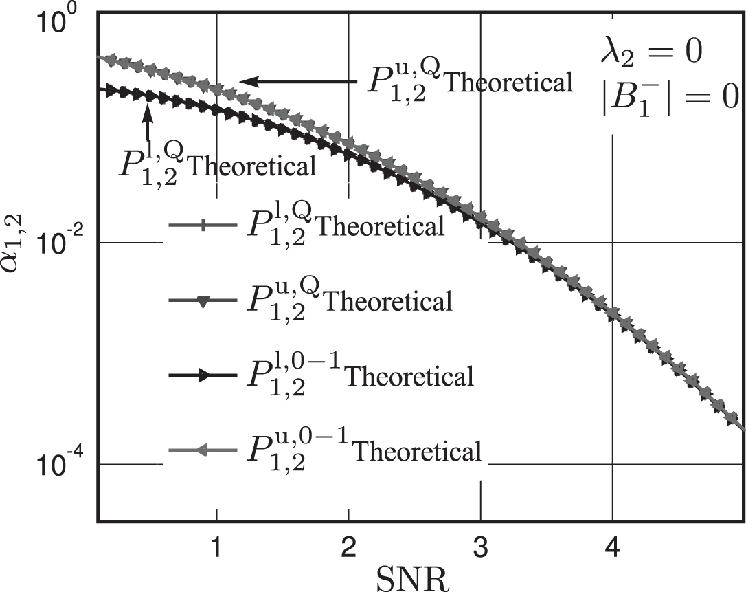
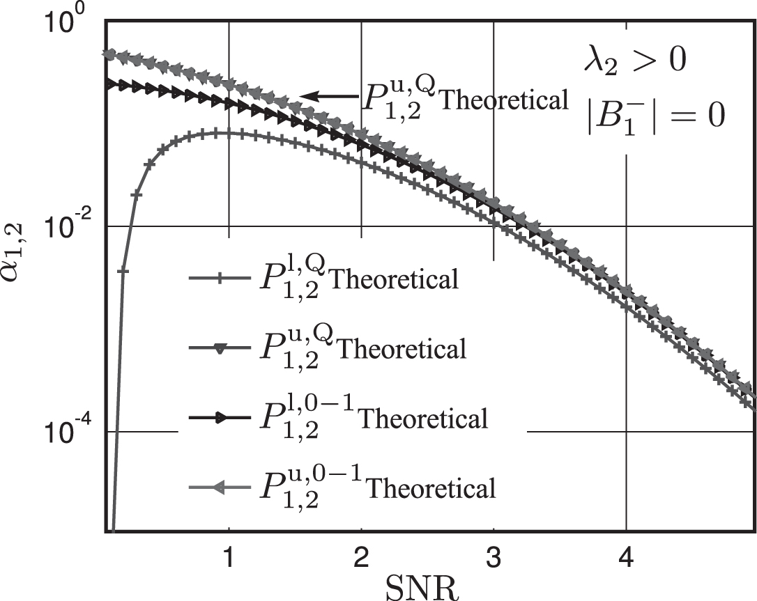
In the third experiment, the influence of parameter geometry on the lower and upper bounds for the proposed test is illustrated by the simulation results based on three network topologies. Each network is composed by three sensors. Specifically, d_1,2 = d_2,3 < d_1,3 in Topology 1, d_1,2 = d_2,3 = d_1,3 in Topology 2 and d_1,2 = d_2,3 > d_1,3 in Topology 3. Without loss of generality, the lower and upper bounds of $α_{1, 2}^{0 - 1}$ and $α_{1, 2}^{Q}$ are observed and a uniform prior distribution is also adopted for the same reason. Note that all results in this experiment are obtained by using a 10⁶-repetition Monte Carlo simulation.

In Fig. 4, since it is calculated that λ₂ = 0 in Topology 1 and a uniform prior distribution is assumed, $P_{1, 2}^{l, Q} = P_{1, 2}^{l, 0 - 1}$ . In addition, it is obtained that $C_{1, 2}^{3} < 0$ , so $| B_{1}^{-} | = 1$ , $P_{1, 2}^{h, Q} > P_{1, 2}^{h, 0 - 1}$ . Then, according to Corollary 2, $P_{1, 2}^{l, Q}$ and $P_{1, 2}^{h, Q}$ do not converge to the same value as SNR increases.

Fig.4

Comparison between the bounds of $α_{1, 2}^{0 - 1}$ and $α_{1, 2}^{Q}$ in Topology 1.

Fig.5

Comparison between the bounds of $α_{1, 2}^{0 - 1}$ and $α_{1, 2}^{Q}$ in Topology 2.

Fig.6

Comparison between the bounds of $α_{1, 2}^{0 - 1}$ and $α_{1, 2}^{Q}$ in Topology 3.

In Fig. 5, because all the $C_{k_{2}, k_{3}}^{k_{1}} = 0$ for 1 ≤ k₁ ≠ k₂ ≠ k₃ ≤ 3 in Topology 2, ${\hat{δ}}^{Q} (X)$ is reduced to ${\hat{δ}}^{0 - 1} (X)$ . Therefore, $P_{1, 2}^{l, Q} = P_{1, 2}^{l, 0 - 1}$ , $P_{1, 2}^{l, Q} = P_{1, 2}^{l, 0 - 1}$ and $α_{1, 2}^{0 - 1} = α_{1, 2}^{Q} \begin{matrix} SNR \to \infty \\ \sim \end{matrix} Q (\frac{SNR}{\sqrt{2}})$ .

In Topology 3, it can be calculated that λ₂ > 0, so $P_{1, 2}^{l, Q} < P_{1, 2}^{l, 0 - 1}$ . Additionally, $C_{1, 2}^{3} > 0$ ,so $| B_{1}^{-} | = 0$ and $P_{1, 2}^{h, Q} = P_{1, 2}^{h, 0 - 1}$ . Therefore, $α_{1, 2}^{0 - 1} \begin{matrix} SNR \to \infty \\ \sim \end{matrix} α_{1, 2}^{Q} \begin{matrix} SNR \to \infty \\ \sim \end{matrix} Q (\frac{SNR}{\sqrt{2}})$ . However, since λ₂ > 0, although it does not ultimately change the asymptotic equivalence between $α_{1, 2}^{0 - 1}$ and $α_{1, 2}^{Q}$ , it makes this phenomenon less remarkable as is shown in Fig. 6.

6 Conclusion

In this paper, the anomaly localization problem in distributed networks is treated as a multiple hypothesis testing problem and then a Bayesian test with a quadratic loss function has been proposed since the quadratic loss function is more suitable than the conventional 0 - 1 one in differentiating the losses caused by different false localizations. The Bayes risk of a test for the MHT problem has been expressed in a closed form as the sum of all misclassification probabilities weighted by the respective prior probabilities. The non-asymptotic bounds of the misclassification probabilities for the proposed test and the Bayesian test with the 0 - 1 loss function have been obtained to analyze their asymptotic performance from which it is derived that the asymptotic performance of the proposed test is influenced by the geometry of the parameter space associated with the hypotheses which further determines the conditional asymptotic equivalence between these two tests.

Acknowledgments

This work was supported by the China Scholarship Council between 2010 and 2014, and is now partly supported by the Fundamental Research Funds for the Central Universities (WUT: 153111003), by the National Science Foundation of China under Grant No. 71371148 and by the Project “the Fundamental Research Funds for the Central Universities” under Grant No. 2010-JL-22.

Footnotes

Appendix A.

Appendix B.

References

Basseville

, Benveniste

, Moustakides

and Rougée

, Detection and diagnosis of changes in the eigenstructure of nonstationary multivariable systems, Automatica23(4) (1987), 479–489.

Basseville

and Nikiforov

, Detection of Abrupt Changes: Theory and Applications, Prentice-Hall, 2010.

Baygün

and Hero

A.O.

, Optimal simultaneous detection and estimation under a false alarm constraint, IEEE Transactions on Information Theory41(3) (1995), 688–703.

Benjamini

and Hochberg

, Controlling the false discovery rate - a practical and powerful approach to multiple testing, Journal of the Royal Statistical Society57(1) (1995), 289–300.

Berger

J.O.

, Statistical Decision Theory and Bayesian Analysis, Springer, 2010.

Chandola

, Banerjee

and Kumar

, Anomaly detection: A survey, Acm Computing Surveys41(3) (2009), 75–79.

Davy

and Godsill

, Detection of abrupt spectral changes using support vector machines an application to audio signal segmentation, IEEE International Conference on Acoustics, Speech, and Signal Processing (ICASSP), 2002, pp. 1313–1316.

Dudoit

and Laan

, Multiple testing procedures with applications to genomics, Springer Science & Business Media, 2007.

Eaton

M.L.

, Multivariate Statistics: A Vector Space Approach, John Wiley and Sons, 1983.

10.

Ferguson

, Mathematical statistics. A decision theoretic approach, Academic Press, 1967.

11.

Fillatre

, Adaptive steganalysis of least significant bit replacement in grayscale natural images, IEEE Transactions on Signal Processing60(2) (2012), 556–569.

12.

Fillatre

and Nikiforov

, Asymptotically uniformly minimax detection and isolation in network monitoring, IEEE Transactions on Signal Processing60(7) (2012), 3357–3371.

13.

Fouladirad

and Nikiforov

, Optimal statistical fault detection with nuisance parameters, Automatica41(7) (2005), 1157–1171.

14.

Gwadera

, Atallah

M.J.

and Szpankowski

, Reliable detection of episodes in event sequences, Knowledge & Information Systems7(4) (2003), 67–74.

15.

Holm

, A simple sequentially rejective multiple test procedure, Scandinavian Journal of Statistics6(2) (1979), 65–70.

16.

Jiang

, Fei

and Huan

, Anomaly localization for network data streams with graph joint sparse PCA, ACM SIGKDD International Conference on Knowledge Discovery and Data Mining, 2011, pp. 886–894.

17.

Johnson

and Kotz

, Continuous multivariate distributions, Wiley, 1942.

18.

Lehmann

E.L.

, Testing Statistical Hypotheses, Wiley, 1968.

19.

Lin

and Bai

, Probability inequalities, Science Press and Springer, 2009.

20.

Miller

R.G.

, Simultaneous statistical inference, Springer, New York, 1968.

21.

Mishra

, Sudan

and Soliman

, Detecting border intrusion using wireless sensor network and artificial neural network, IEEE International Conference on Distributed Computing in Sensor Systems Workshops, 2010, pp. 1–6.

22.

Zhang

, Fillatre

and Nikiforov

, Bayesian test for multiple hypothesis testing problem with quadratic loss, Adaptation and Learning in Control and Signal Processing, 2013, pp. 506–511.