Non-destructive low-cost approach for fuzzy classification of tomato images based on firmness prediction using regression

Abstract

Non-destructive techniques such as hyperspectral imaging, backscattering imaging are the advanced techniques used for predicting mechanical properties of horticulture products. They show relatively good performance but at the expense of costly measuring setups. This application-oriented paper investigates the feasibility of employing simple digital color camera imaging for prediction and fuzzy classification of firmness of tomatoes. Images acquired using digital color camera are preprocessed and subject to texture analysis in order to extract the number of features. The proposed approach exploits four texture feature extraction algorithms: three are based on statistical techniques viz. first order statistics (FOS), gray level co-occurrence matrix (GLCM), gray level run length matrix (GLRLM), and one is based on transform-based technique viz. wavelet-transform. Out of all extracted features, redundant features are eliminated using various attribute selection methods. Subsequently, prediction models are built and analyzed using regression analysis. Sample space has been split into two sets; 80% training and 20% testing data having tomatoes with almost identical formation. Experimental results illustrates that RBF regression gave the lowest RMSE of 0.174 and highest prediction correlation coefficient of 0.929 for wavelet feature set. Grounded on the prediction model, fuzzy rule based classification (FRBC) is proposed to classify tomatoes into three firmness categories soft, medium, and hard. Accuracy statistics of the proposed FRBCS are compared with the state-of-the-art result and highest classification accuracy of 92.68% is achieved by proposed FRBCS. The results exhibit the possibility of using a digital color imaging system for firmness estimation and further for classification.

Keywords

Image texture analysis Tomato firmness fuzzy rule based classification system RBF regression machinevision

1 Introduction

Tomato is one of the most widely consumed fresh vegetables all over the world. Acceptability of tomato is based on two factors, external qualities including color, size, shape, and internal qualities including firmness, soluble solid content, acid, and juice. External feature color and internal feature firmness are the most imperative factors observed by the consumer (wholesaler or retailer) for determining the quality of tomatoes [1]. Color is the indicator of the ripeness stage of tomato whereas firmness serves as the measure for its textural quality. Texture has high influence on quality and consumers’ preference. Typically, it is preferred that whilst being ripe, the fruit preserves a high degree of strength to protect the fruit from damage such as breaking during handling and transport.

In recent years, computer vision has been widely used for the quality inspection of fruits and vegetables [2]. Some of the advantages that favor the application of computer vision to agricultural problems include speediness, non-destructive evaluation possibilities, and ease. The increased demand for high quality vegetable and food products and their safety compels the growth of accurate, fast, and objective quality determination of food and agricultural products [3].

Texture is an imperative image feature that has been applied significantly in the food industry for food and crop quality estimation [4]. Recent applications of texture-analysis techniques in the food industry have determined the mechanical properties of food materials non-destructively [5]. The advanced techniques show relatively good performance in predicting mechanical properties of horticulture products [6 –12]. However, the requirement of a distinctive imaging apparatus and cost is the major drawback concerning these techniques [13]. Simple imaging techniques using digital camera, scanners have also been adopted for products such as chicken nuggets [14], bread [15], and tea [4]. Researchers have obtained good performance in envisaging the mechanical properties of the products using image texture-based analysis techniques such as wavelet-transform, or GLCM. Significant work has not been done for exploring simple imaging technique for estimating the mechanical properties of tomato using texture-based analysis. Authors Sehgal et al. [16] explored the viability of using digital camera for firmness estimation of tomatoes. Multiple linear regression (MLR) analysis was done to establish the relation between the instrumental firmness and texture features extracted from the texture analysis of tomato images captured. The results showed the satisfactory performance with correlation of 0.89 but the validation test was not conducted on independent sample sets.

To measure the food texture using non-destructive test i.e. imaging, the texture properties must be measured by well-established reference methods such as compression test (universal testing machine (UTM)) or puncture/penetration test (texture-analyzers) [17, 18] along with the measurement of non-destructive methods. After this, results of both the experiments are given as an input to various statistical methods or artificial neural networks (ANNs) for developing prediction models.

Machine vision (MV) provides a mechanism in which human process is simulated artificially. Until date, MV has been widely applied to solve various agricultural problems, ranging from simple quality evaluation [19, 20] to complex robot-steered applications [21 –23]. Consumers on the other hand, grade quality of food products in a fuzzy way according to their senses such as sight, touch, smell etc.

Therefore, the objective of the present work is two-fold i.e. to predict the firmness of tomatoes non-destructively and classify them into logical classes using fuzzy logic. Since imaging is generally non-destructive reliable and rapid [24], henceforth, the proposed work is non-destructive in nature. Different image texture analysis techniques including statistical and transform-based techniques are examined. In addition, for exhibiting the prediction model, feature selection is performed using greedy approach, evolutionary search, and particle swarm optimization (PSO) search before applying regression analysis. For regression analysis, polykernel-based Gaussian process, RBFkernel-based Gaussian process, RBF regressor (radial basis function), polykernel-based SMOreg, RBFkernel-based SMOreg, and PLS regression approaches are compared and analyzed to produce the texture feature set that best predicts the firmness. After building the prediction model, FRBC model is proposed for classifying the firmness into three classes soft, medium, and hard. Hence, the viability of using simple imaging systems in real-time applications for tomato firmness prediction and fuzzy classification based on predicted firmness has been explored by exploiting the texture-based feature analysis.

2 Material and methods

2.1 Data set

In the experiments, around 150 samples of tomatoes were collected from an open farm during daytime under natural lighting conditions. Samples that were free from visual defects were selected for experiments.

2.2 Objective/instrumental texture evaluation

After acquisition of images, samples were subjected to penetration test for firmness measurement using TA.XT2 plus texture analyzer by Stable Micro Systems [18, 25]. Calibration of instrument was done (settings as shown in Table 1) and tests were carried out for the whole fruit. Penetration test is defined as one in which the depth of penetration or the time required to reach a certain depth is measured under a constant load. While performing experiments characteristic force-deformation curves are obtained as force-time graphs. Figure 1 displays the force-time graph obtained for a batch of six tomato samples. When the probe punctures through the skin and begins to penetrate into sample flesh, it is often called as “Bio yield point (BYP)”. The BYP occurs when the probe begins to penetrate into the fruit causing irreversible change in the sample being tested. The force profile after this point signifies penetration into the underlying flesh of the fruit and indicates that this is substantially softer than the fruit. Force values corresponding to BYP are noted as Newton (N). Table 2 reports the statistical data (few batches) for firmness of tomatoes measured using TA.XT2 analyzer.

Table 1
Texture analyzer settings for the experiments

Test Penetration Test

Accessory P/3 (3 mm cylindrical probe) using

50 kg load cell

Mode Compression

Option Return to Start

Pre-Test Speed 1 mm s^–1

Test Speed 2 mm s^–1

Post-Test Speed 10 mm s^–1

Target Mode Distance

Distance 15 mm

Trigger Type Auto –0.049 N

Tare Mode Auto

Data Acquisition Rate 200 points per second

Test	Penetration Test
Accessory	P/3 (3 mm cylindrical probe) using
	50 kg load cell
Mode	Compression
Option	Return to Start
Pre-Test Speed	1 mm s^–1
Test Speed	2 mm s^–1
Post-Test Speed	10 mm s^–1
Target Mode	Distance
Distance	15 mm
Trigger Type	Auto –0.049 N
Tare Mode	Auto
Data Acquisition Rate	200 points per second

Fig.1

Force-deformation curve obtained from the penetration test.

Table 2

Statistical data (few batches) for measured instrumental firmness using TA.XT2 analyzer

Batch	Skin Strength Force(N)
	Average	S.D.	Coef. of Variation
Batch 1	16.702	4.208	25.192
Batch 2	14.22	3.168	22.277
Batch 3	15.184	3.626	23.883
Batch 4	16.455	2.294	13.94
Batch 5	19.704	2.785	14.136
Batch 6	17.337	2.856	16.473

2.3 Image acquisition and pre-processing

Images of around 150 tomato samples were taken without any artificial lighting system. A CCD camera (Nikon Coolpix S220V1.0, resolution 3648×2736 pixels) has been used for capturing the tomato images. As the size of the captured images captured is very large (3648×2736 pixels), they are first scaled down to 1/8th of their size to expedite the calculations. Image processing is done using MATLAB R2009a. Hereafter, segmentation process [26] on captured images is applied to separate out the region of interest (ROI) from the background.

2.4 Image texture analysis

Methodologies used for texture analysis are broadly classified into four categories: statistical, structural, model-based, and transform-based or filter based. Among these, statistical texture [27] is the most widely used one in the food industry for its high accuracy and less computation time. Transform-based texture is also commonly used technique while model-based and structural texture technique are rarely used in the food industry [28].

Apart from features extracted in the work done [16] one more statistical texture-based features viz. gray level run length matrix (GLRLM), is also considered here to process the captured images. All these techniques are computationally efficient than other statistical and transform-based techniques [8]. Brief description of these techniques is provided in the following subsections.

2.4.1 First order statistics (FOS)

First order statistics are the most elementary texture features extraction methods based on the probability of pixel intensity values occurring in digital images. Before extracting texture features, it is essential to equalize the histogram of the image pixels to reduce the influence of changing illumination. First, the histogram of gray level images obtained in Section 2.3 is extracted. They are then normalized according to the formula given by Equation (1). $P (x_{i}) = H (x_{i}) / N$ (1)

Where, H (x_i) is the image histogram, P (x_i) is the normalized histogram, and N is the total number of elements in the image matrix. Ten statistical features mean (μ), standard deviation (σ), skewness for red component (skewR), skewness for green component (skewG), skewness for blue component (skewB), entropy, kurtosis for red component (kurtR), kurtosis for green component (kurtG), kurtosis for blue component (kurtB), and coefficient of variation (Cv) were extracted from each image using its normalized histogram. The list of features is presented inTable 3.

Table 3

Texture features using First order statistics (FOS) for image histogram

Feature Name	Formula
Mean gray level	$\sum_{i = 1}^{N} x_{i} p (x_{i})$
Standard deviation	$σ = \sqrt{\sum_{i = 1}^{N} (x_{i} - μ)^{2} p (x_{i})}$
Skewness	$\frac{1}{σ^{3}} \sum_{i = 1}^{N} (x_{i} - μ)^{3} p (x_{i})$
Entropy	$- \sum_{i = 1}^{N} p (x_{i}) {log}_{2} p (x_{i})$
Kurtosis	$\frac{1}{σ^{4}} \sum_{i = 1}^{N} {(x_{i} - μ)}^{4} p (x_{i})$
Coefficient of variation	σ/μ

2.4.2 Gray level co-occurrence matrix

The gray level co-occurrence matrix (GLCM) is a statistical and one of the most commonly used texture feature extraction method [15]. For examining texture, this method considers the spatial relationship of pixels. It is an n×n matrix where n is the number of gray levels in an image. Each matrix entry describes the number of occurrences of two gray levels given a specific offset. These offsets define pixel relationships of direction, θ and distance, d. The comparison of the GLCM can be done with fourteen statistical features as suggested by Haralick [27]. To reduce the computational cost, only four commonly used features contrast, correlation, energy, and homogeneity were selected. The tomato images were analyzed using the distance, d = 1 pixel with angles θ = 0, 45, 90, and 135. Thus, 16 features (4 directions X 4 features) were extracted from each tomato image.

2.4.3 Gray level run length matrix (GLRLM)

This technique registers the roughness of a texture in specified directions based on the number each gray level appearing in the image. A GLRLM is a matrix in which each element a(i, j) determines the total number of occurrence of run lengths j in the gray level i in specified direction d. Run length matrices at four directions d = 0, 45, 90, and 135 were extracted for each captured image. 11 texture descriptors for GLRLM in each direction [29], were calculated to capture the texture properties. Thus, 44 features (11 features X 4 directions) were obtained from each tomato image.

2.4.4 Wavelet transform

Wavelet transform has been used for analyzing the texture of agricultural materials [4]. Mallat [30] developed an efficient way of implementing discrete wavelet transform (DWT) using filter banks that decomposes an image into multiple wavelet components. At each level of decomposition, two sets of coefficients are obtained, approximations and details (horizontal, vertical, diagonal), which in total make four coefficients. The approximations are in high-scale and low frequency components of the signal. Whereas, the details are in low-scale and high frequency components of the signal. Captured images were subject to four levels of wavelet decomposition using a fourth-order Daubechies mother wavelet (Db4) [31]. To determine optimum level of decomposition, images at each level of decomposition were compared to the original images. As shown in Fig. 2, afterwards fourth level of decomposition the extent of down sampling increases, causing lower resolutions in the samples. Thus, the wavelet coefficients from first level to the fourth level of decomposition were considered. At all the levels of decomposition, approximation coefficients and detail coefficients for horizontal, vertical, and diagonal orientations were obtained. Three statistical descriptors including mean, standard deviation, and entropy were extracted from each level of decomposition. Total of 48 features (3 statistical descriptors X 4 wavelet coefficients X 4 decomposition levels) were obtained from the DWT of each image.

Fig.2

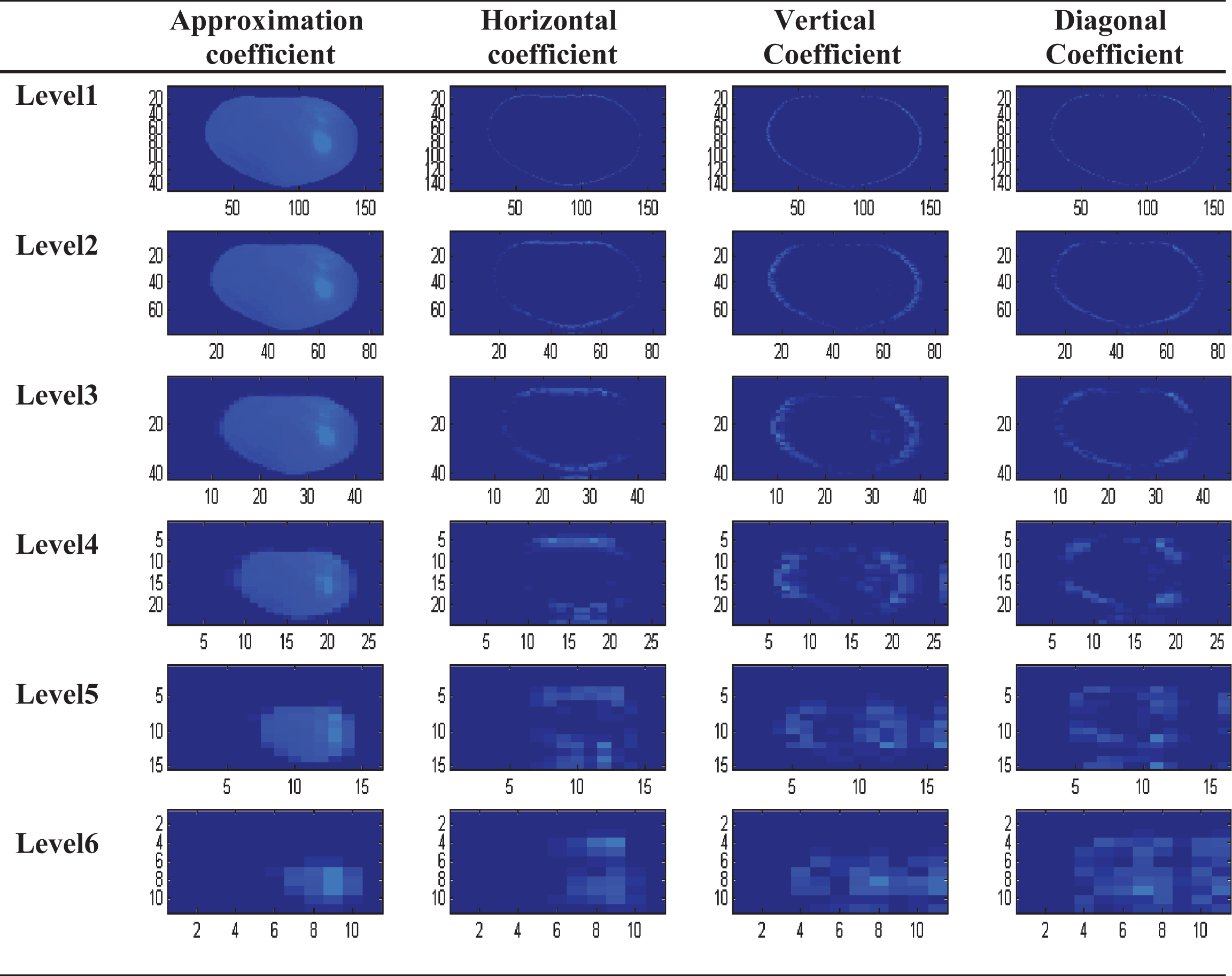
Six level Wavelet decomposition of tomato sample image using Db4 mother wavelet.

2.5 Feature/Attribute selection

The feature extraction process leads to data sets with number of inputs as 7 for FOSH, 16 for GLCM, 44 for GLRLM and 48 for wavelet. Large number of model inputs may lead to increase in execution time and consequently reduces the predictive accuracy. Attribute selection methods such as greedy stepwise algorithm, evolutionary search, and PSO search decipher these problems by eliminating redundant features. In this study, all these three methods were compared and analyzed to obtain the optimum feature set that will be further used for predicting the firmness.

2.6 Prediction model

To ensure that models were not over-fitted and prediction results truly represent the model performance, the samples were first divided into two separate parts randomly. The first part (or 80% of all samples) was used for training, 20% of all samples were used for independent test or prediction. To select the best prediction model from the training samples, six state-of-the-art regression techniques; polykernel-based Gaussian process, RBFkernel-based Gaussian process, RBF regressor (radial basis function), polykernel-based SMOreg, RBFkernel-based SMOreg and partial least square (PLS) regression were compared and analyzed. The models were evaluated using root mean squares errors for prediction (RMSEP). $RMSE = \sqrt{\frac{\sum_{i - 1}^{i = n} (x_{i}^{'} - x_{i})^{2}}{n}}$ (2)

Where $x_{i}^{'}$ is the actual value, x_i the predicted value, and n is the number of samples in prediction stage. In addition, correlation coefficient for prediction (R_p) has also been calculated. Since processing time is a significant factor in real-time applications, it was recorded to be used as an evaluation criterion for each feature extraction technique. WEKA was used for statistical analysis in a laptop computer with this configuration: Core 2Duo CPU, 1.53 GHz, 2 GB RAM, Windows 7 OS.

Firmness of tomato estimated through prediction model is in the form of crisp value. However, user tries to explain the firmness of fruit in a vague manner such as soft, slight soft or slight hard but medium or hard and so on. Therefore, this problem can be exhibited precisely using fuzzy logic.

3 Firmness classification using fuzzy rule based decision system

To fuzzify the crisp values and represent them as classes, we earlier proposed a technique FRBCS [32] that provides a self-reliant decision-making resource for the harvesting robot to classify the tomatoes based on ripeness using color as their attribute without the need of any human expert. The FRBCS proposed earlier has been deployed here to classify the tomatoes based on their firmness. It depicts the problem in a manner closer to human thinking process. Figure 3 displays the flowchart for the classification using fuzzy rule based decision system. Detailed discussion of the steps from the perspective of classifying tomato images based on firmness is given as follows.

Fig.3

Flowchart for the classification using fuzzy rule based decision system.

Step 1: Define the input and output attributes.

The input is the training dataset i.e. the predicted firmness (“predFirm”) and their corresponding classes. The output attribute i.e. class attribute has three classes. Class C1 represents the hard or firm class (hard), C2 is the medium (med) class, and C3 is the soft class (soft).

Step 2: Feature space fuzzy partitioning

By outlining the proper interval values and boundaries of each region, fuzzy regions for the input attribute ‘predFirm’ are created. Initial intervals for the fuzzy regions in the universe of discourse X = [Xmin, Xmax] are given by Equations (3 and 4). $Interval (A) = {u_{1}, u_{2}, u_{3}, \dots, u_{max}}$ (3)

Where, u₁ = X_min, u₂ = Incr (A) , …, and u_max = Incr (A) * k and u_max-1 < A^max ≤ u_max

X_min= minimum value of X, X_max= maximum value of X $Incr (A) = [\frac{A^{\min} + A^{\max}}{| A |} * w]$ (4)

A^min= minimum value of A.

A^max= maximum value of A.

|A| = number of distinct values of A

w = is the positive integer user-defined weight.

k = is the positive integer (1, 2, 3 ... n)

In the proposed system, ‘A’ characterizes the feature vector “predFirm”, which is the predicted firmness. X = [0 ... 23.11] is the universe of discourse of attribute A. In accordance with the values obtained (as discussed in section 2) for input attribute A, A^min= 5.44, A^max= 23.11, |A| = 133. ‘w’ is a positive integer positioned to control the number of regions that needs to be created. Using Equation (4), for w = 15, Incr(A) = 3.22 and for w = 30, Incr(A) = 6.44, the choice w = 15 has been experimentally found to be the optimum choice as it will create reasonable number of fuzzy regions. Now according to Equation (3), u₁ = 0, u₂ = 3.22 * 1, u₃ = 3.22 * 2, u₄ = 3.22 * 3, u₅ = 3.22 * 4, u₆ = 3.22 * 5, u₇ = 3.22 * 6, u₈ = 3.22 * 7 u₉ = 3.22 * 8. The last unit will be u₉ = 3.22 * 8, since it satisfies the condition: 22.54 < A^max = 23.11 ≤ 25.76 as given in Equation (3). However, for k = 10 the condition is not satisfied because 25.76 ≮ A^max = 23.11 ≤ 28.98.

Henceforth, we get the initial intervals for the input attribute “predFirm” as Interval (predFirm) = {0, 3.22, 6.44, 9.66, 12.88, 16.1, 19.32, 22.54, 25.76}.

Divergent values of input attribute predFirm are now denoted by the set of fuzzy regions {R₁, R₂ … R_k}. Any kth region R_k is defined as the set of three parameters as $R_{k} = {R_{k}^{l}, M_{k}, R_{k}^{u}}$ , where, $R_{k}^{l}$ is the lower limit value, M_k is the modal value, and $R_{k}^{u}$ is the upper limit value. The initial lower parameter, $R_{k}^{l}$ and upper parameter, $R_{k + 1}^{u}$ obtained for the adjacent fuzzy regions R_k and R_k+1 respectively are now tuned based on the overlap degree between them. Overlap (R_k, R_k+1) is the metric which gives the degree of overlay between the adjacent fuzzy regions R_k and R_k + 1 [32].

The overlap degree for the input attribute “predFirm” between the adjacent regions is given in Table 4. In this table, column “Region” shows the initial regions for the input attribute “predFirm”, column “Classes” specifies the set of classes covered by the respective regions.

Table 4

Overlap degree between the adjacent regions

A	Region R_k	Classes	Overlap (R_k, R_k + 1)	$R_{k}^{u}$	$R_{k + 1}^{l}$	M _k	merge(R_k, R_k+1)
predFirm	R1	{C1}	(R1,R2) = 0.5	$R_{1}^{u} = 8.05$		M₁ = 3.22
					$R_{2}^{1} = 4.83$
	R2	{C1, C2}	(R2,R3) = 0.3	$R_{2}^{u} = 10.63$		M₂ = 8.05
					$R_{3}^{l} = 8.69$
	R3	{C2, C3}	(R3,R4) = 0.5	$R_{3}^{u} = 14.49$		M₃ = 11.27
					$R_{4}^{l} = 11.27$
	R4	{C3}	(R4,R5) = 1			M₄ = 17.79
	R5	{C3}	(R5,R6) = 1
	R6	{C3}	(R6,R7) = 1				Merge(R4,R5,R6,R7)
	R7	{C3}

The membership degree ‘μ’ of an input value, say x, is estimated by a triangular MF for computing the degree of value ‘x’ that belongs to region R_k [32]. Figure 4 shows the partitions (initial MFs) obtained for the predFirm attribute without overlapping & Fig. 5 shows the fuzzy partitions (final MFs with overlapping) attained between the regions respectively.

Fig.4

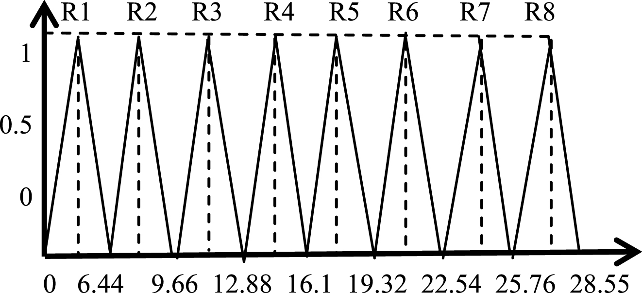
Initial MFs without overlapping.

Fig.5

Final MFs with overlapping.

Table 5 below displays few of the fuzzified values from the training dataset. Grounded on their degree of membership, crisp values are transformed to linguistic variables. Region names soft corresponds to region R1, soft-med to R2, med-hard to R3, and hard to R4. Column “predFirm” shows the crisp values of firmness from the training dataset and column “Region” shows the linguistic variables to which they are mapped according to their degree of membership.

Table 5

Crisp values changes to fuzzy values (linguistic variables)

predFirm	Region	predFirm	Region	predFirm
17.04	hard	10.27	med-hard	7.494
14.23	hard	12.32	med-hard	8.135
17.88	hard	20.86	hard	9.697
12.06	med-hard	9.202	soft-med	9.021
14.76	hard	10.95	med-hard	9.028
9.337	soft-med	17.04	hard	9.587

Step 3: Generate rule base using Decision Trees.

As described in [32], a rule bas e is formed using decision tree (DT) to produce the rules automatically from the feature set, which helps in eradicating the need of human expert for creating the rules. Rules obtained by traversing each branch of the decision tree are:-

If predFirm = soft then class = soft

If predFirm = soft-med then class = soft

If predFirm = med-hard then class = med

If predFirm = hard then class = hard

Step 4: Fuzzy Inference Process

Subsequently, next step is to feed the membership function (step 2) and generated “if-then” rules (step 3) to the fuzzy inference system (FIS). Output of the system is the firmness class of the tomato. Outline of the proposed fuzzy rule based classification system is shown in Fig. 6.

Fig.6

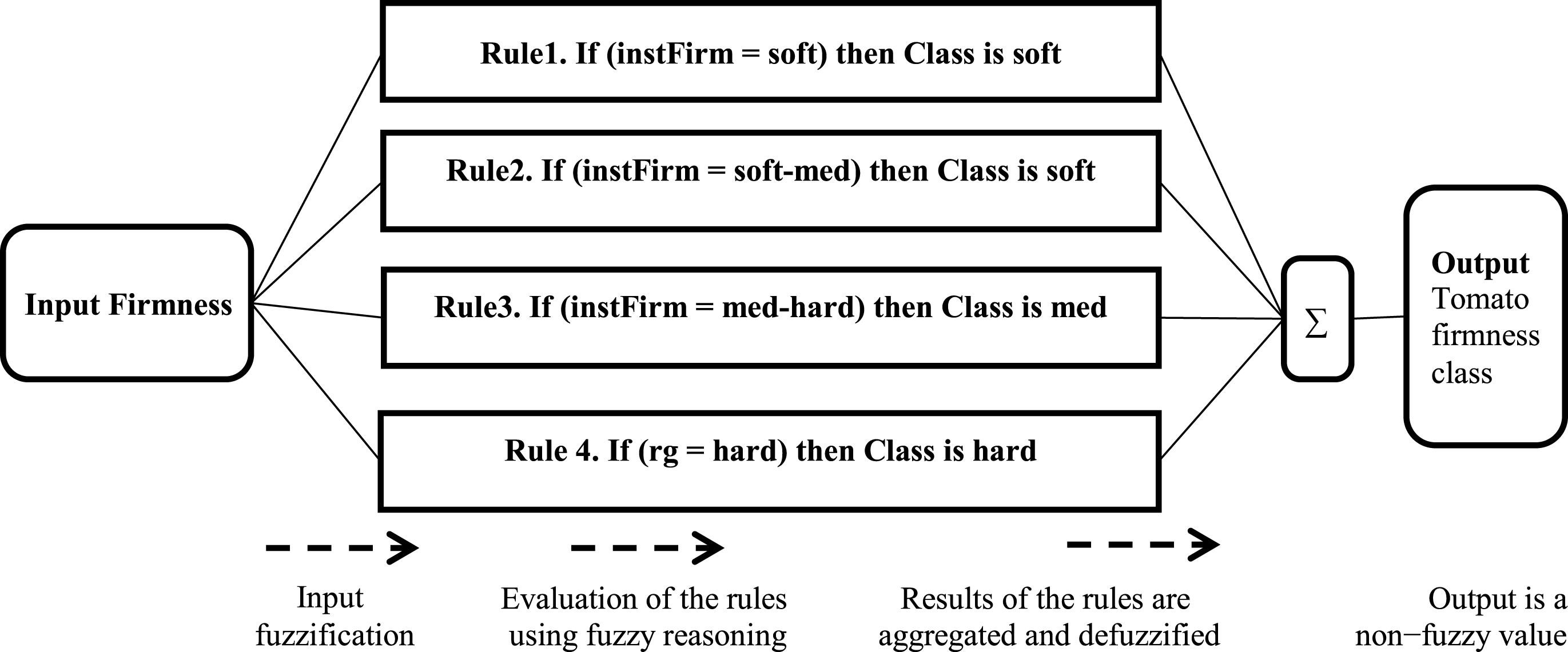
Structure of the proposed FRBCS.

4 Results and discussion

4.1 Firmness prediction

In real-time applications, such as grading/sorting machines, two factors are important: prediction accuracy and processing time. To compare the capability of different texture techniques for real-time applications, processing time during feature extraction process for each technique was recorded. Figure 7 illustrates the time achieved by various texture methods on the study data set. Results show that GLRLM is unsuitable for real-time systems since it requires considerable much time for implementation. On the other hand, FOSH, GLCM, and wavelet, and were the fastest techniques because their processing time was less than 0.5 s.

Fig.7

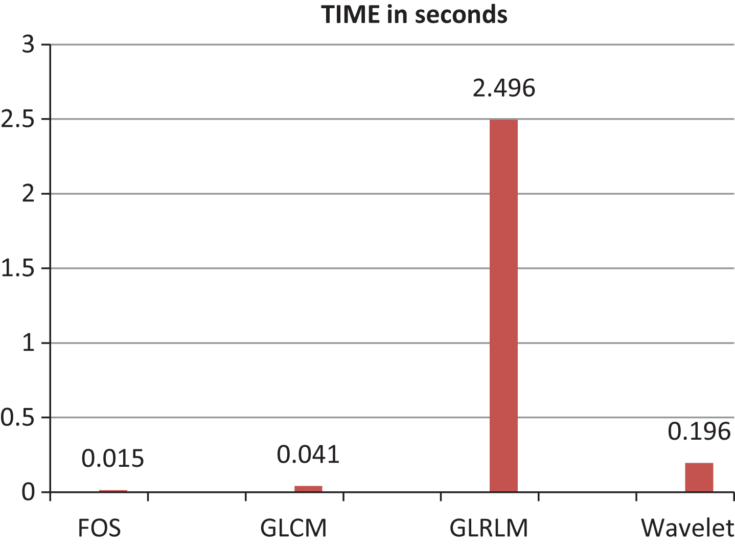
Time comparison (in seconds) of individual feature set models.

Table 6 shows the list of top texture analysis features obtained by three feature (attribute) selection methods for tomato. Different numbers of features were selected by three attribute selection techniques. This process considerably reduced the size of feature vectors.

Table 6

Variable selection using greedy, Evolutionary search and PSO search algorithm

FOS	GLCM	GLCM	GLCM	GLRLM	GLRLM	GLRLM	Wavelet	Wavelet	Wavelet
	greedy	Evol	PSO	greedy	Evol	PSO	Greedy	Evol	PSO
Coeff_variation	corr45	corr45	corr0	lgre45	lre0	hgre0	vm1	vm1	vm1
SkewB	energy45	energy45	corr45	sre90	hgre0	srlge0	aSD1	vSD1	aSD1
	hom45	hom45	corr135	rp90	lrhge0	lrhge0	vSD1	hm2	vSD1
			energy0	lgre90	lgre45	sre45	dSD1	hSD2	dSD1
			energy45	srlge90	lrhge45	lre45	hEntropy1	vSD2	hEntropy1
			hom0	sre135	glnu90	srhge45	vm2	hEntropy2	vEntropy1
			hom45	rlnu90	sre90	vSD2	am3	dSD2
					rp90	lgre90	hEntropy2	vSD3	hEntropy2
					hgre90	srlge90	vSD3	dSD3	am3
					srlge90	sre135	am4	dEntropy3	vSD3
					srhge90	lre135	vSD4	vSD4	hEntropy3
					sre135	srhge135	dSD4		vSD4
					lre135		dEntropy4		hEntropy4
					glnu135
					hgre135
					srlge135
					lrhge135

Statistical measures of individual texture-based feature models for predicting firmness of tomatoes by six regression techniques are presented in Tables 7–10.

Table 7

RMSE and R value for Prediction model using FOS texture feature set

	FOS
	Greedy/Evolutionary search/PSO Search
	RMSE	R
Gaussian Polykernel	0.249	0.773
Gaussian RBFkernel	0.308	0.837
RBF Regressor	0.260	0.739
SMO PolyKernel	0.235	0.845
SMO RBFKernel	0.260	0.8329
PLS regression	0.218	0.855

Table 8

RMSE and R value for prediction model using GLCM texture feature set

	GLCM
	Greedy		Evolutionary search		PSO Search
	RMSE	R	RMSE	R	RMSE	R
Gaussian Polykernel	0.210	0.792	0.210	0.792	0.211	0.793
Gaussian RBFkernel	0.301	0.785	0.301	0.785	0.260	0.786
RBF Regressor	0.232	0.843	0.232	0.844	0.231	0.834
SMO PolyKernel	0.288	0.804	0.288	0.804	0.290	0.803
SMO RBFKernel	0.197	0.785	0.197	0.785	0.175	0.800
PLS regression	0.244	0.818	0.244	0.818	0.255	0.868

Table 9

RMSE and R value for prediction model using GLRLM texture feature set

	GLRLM
	Greedy		Evolutionary search		PSO Search
	RMSE	R	RMSE	R	RMSE	R
Gaussian Polykernel	0.256	0.7217	0.254	0.884	0.254	0.860
Gaussian RBFkernel	0.335	0.901	0.315	0.828	0.316	0.870
RBF Regressor	0.200	0.889	0.219	0.875	0.196	0.891
SMO PolyKernel	0.243	0.897	0.211	0.897	0.236	0.834
SMO RBFKernel	0.243	0.899	0.241	0.865	0.244	0.876
PLS regression	0.262	0.873	0.224	0.871	0.250	0.851

Table 10

RMSE and R value for prediction model using wavelet texture feature set

	Wavelet
	Greedy		Evolutionary search		PSO Search
	RMSE	R	RMSE	R	RMSE	R
Gaussian Polykernel	0.1948	0.9018	0.204	0.901	0.193	0.906
Gaussian RBFkernel	0.306	0.889	0.322	0.907	0.324	0.8948
RBF Regressor	0.207	0.902	0.231	0.849	0.174	0.929
SMO PolyKernel	0.214	0.898	0.203	0.902	0.207	0.890
SMO RBFKernel	0.215	0.898	0.216	0.907	0.218	0.901
PLS regression	0.208	0.899	0.217	0.890	0.216	0.887

Comparing the performance of attribute selection methods, PSO search yielded in minimum RMSE 0.218, 0.175, 0.196, and 0.174 for all the regression techniques for FOS, GLCM, GLRLM, and wavelet feature set model respectively. For FOS feature set model, all three attribute selection techniques selected the same variable, henceforth, RMSE and R is same in all the cases (Table 7). Statistics in Table 7 shows that PLS Regression gave the minimum RMSE of 0.218 and maximum correlation coefficient (Rp) of 0.855 for FOS features set (Fig. 8(a)) followed by 0.869 for GLCM feature set shown in Table 8. Whereas, for GLRLM feature set RBF regressor gives the good performance (Rp = 0.891341 (Table 9)) followed by the wavelet feature set Rp = 0.928581 (Table 10). Figure 8 demonstrates the graph of RMSE comparison for prediction model using FOS, GLCM, GLRLM, and wavelet texture feature set.

Fig.8

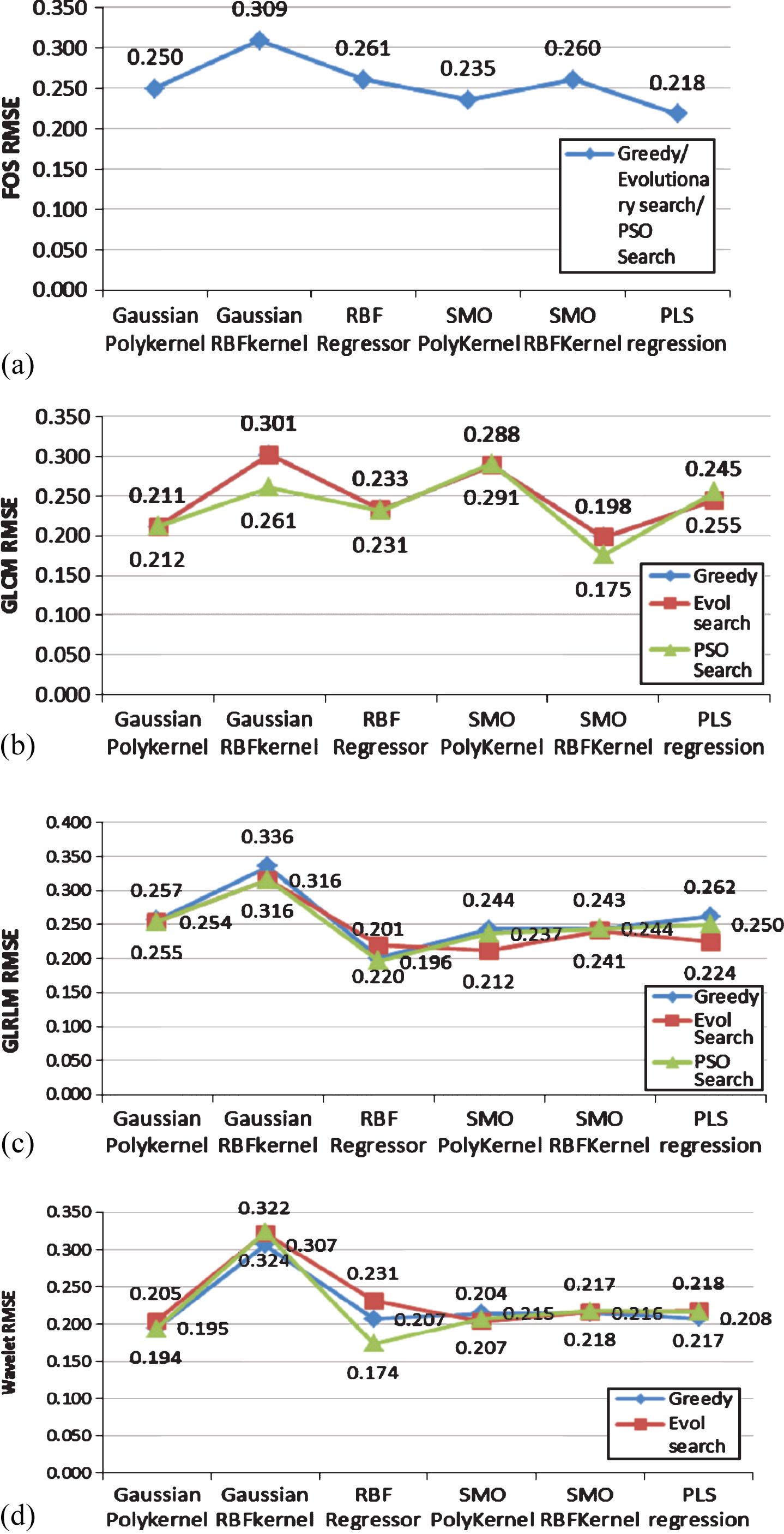
Graphs showing the RMSE comparison for prediction model using (a) FOS texture feature set (b) GLCM texture feature set (c) GLRLM texture feature set (d) wavelet texture feature set.

Gray portions highlight the techniques that attained lowest RMSE and highest R for a particular feature set. From the above tables it can be observed that PLS regression and RBF regressor performed almost equally for all the four feature sets. In addition, attribute selection performed through PSO search resulted in best accuracy statistics for all the regression techniques.

Since, PSO search ascertains to be the best feature selection criteria, all the regression techniques are compared against their R-value for four feature sets based on PSO search. It has been illustrated graphically through Fig. 9. From graph, it can be realized that RBF regression gave the highest prediction correlation coefficient of 0.929 for wavelet-transform feature set. In addition, RBF regression gave lowest RMSE of 0.174 for wavelet-transform feature set (Fig. 8). Hence, wavelet-transform can be selected as the best texture-based technique for analysis of images captured using digital camera because of their consistency in firmness prediction performance. Reason can be attributed to the capability of wavelet transform in analyzing the texture values of an image up at different scales. It gives more detailed information that relates well with mechanical firmness of the tomato. The decomposed sub-images at different scales offer unique textural features, which may not be visible in the original images and thus eliminates the redundancy of resolutions. While, statistical approaches are restricted only to spatial distribution analysis of textures.

Fig.9

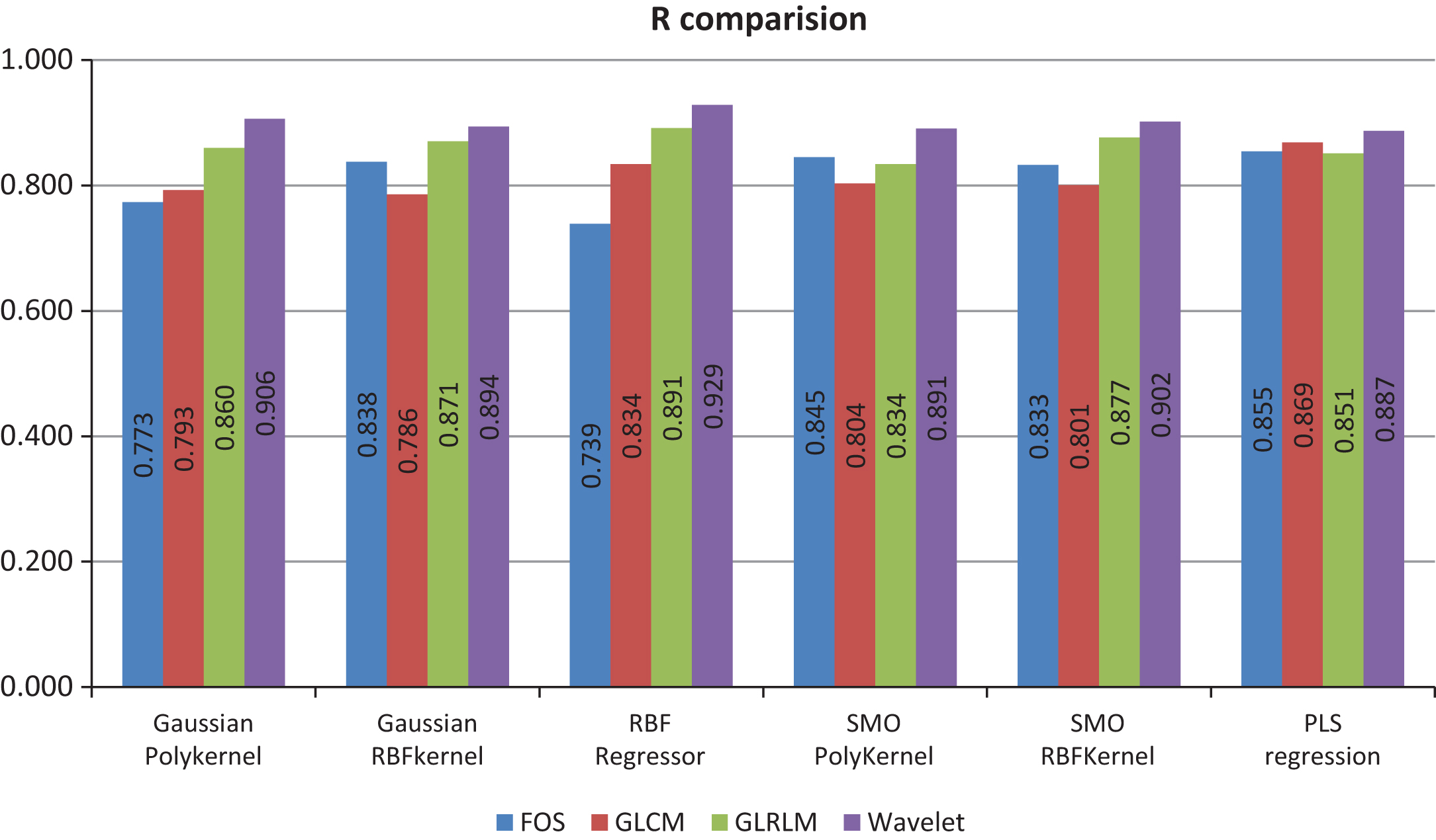
Correlation coefficient (R) comparison of FOS, GLCM, GLRLM, wavelet feature set obtained using PSO search.

4.2 Classification results using proposed FRBCS for tomato firmness

For assessing the accuracy of proposed FRBCS for firmness classification, the sample dataset of tomato images is randomly split into two partitions viz. 80% of the dataset is used for training and 20% of the dataset is used for testing. Results obtained are listed in Tables 11–13. Table 11 shows the classification accuracy, and kappa statistics of the system. Kappa Statistic [33] is a measure of the agreement between the predicted and the true class, where value of 1.0 signifies complete agreement. For this purpose, a higher value was expected for a classifier having more coinciding predicted and actual values.

Table 11
Evaluation metrics for the proposed FRBCS

Total number of instances 133

Accuracy 92.68%

Incorrectly classified Instances (in %) 7.31%

Kappa statistics 0.9265

Table 12

Detailed Accuracy by class

Class	TP Rate	FP Rate	Precision	Recall	F-Measure
soft	0.929	0.074	0.86	0.929	0.892
medium (med)	0.86	0.038	0.929	0.86	0.892
hard	1.00	0.00	1.000	1.00	1.000

Table 13

Performance comparison of proposed FRBCS for firmness with state-of-art learning algorithms

	Accuracy (%)	Kappa statistic
Naíve Bayes	87.65	0.814
SVM	90.86	0.862
MLP	90.66	0.859
RandomTree	82.55	0.737
Proposed FRBCS	92.68	0.927

Table 12 displays the detailed accuracy for each of the three classes. For every class, True Positive rate (TP), False Positive Rate (FP), Precision, Recall, and F-measure is calculated.

From Table 12, we can observe that tomato images are correctly classified with the true positive rate of 1.0 for the hard class. However, false positive rate of 0.038 and 0.074 can be observed in the soft and med class. The reason behind this is that some tomatoes that belong to soft class were misclassified as medium and vice-versa. This error resulted in dropout in precision for both soft and medium class.

The proposed FRBCS for firmness is compared with other state-of-art learning algorithms such as NaiveBayes, SVM, Multilayer perceptron (MLP), decision tree, and RandomTree. Table 13 reports the performance statistics for proposed FRBCS and other state-of-art learning algorithms.

Figure 10 illustrates the comparison of the proposed system and other learning algorithms based on their classification accuracy and kappa statistics. From the graph, it can be observed that classification accuracy achieved by SVM and MLP is 90.86 and 90.66 respectively, which is comparable to the proposed algorithm i.e. 92.68. However, kappa statistics of proposed algorithm is much higher (0.927) as compared to SVM (0.862) and MLP (0.859). Highest classification accuracy of 92.68% (shown as bar graph) and kappa statistics of 0.93 (shown as line graph) is achieved by proposed FRBCS for firmness. This signifies that the settlement amongst the predicted and actual class is much improved in case of proposed FRBCS indicating the good classification competency of the proposed FRBCS for firmness.

Fig.10

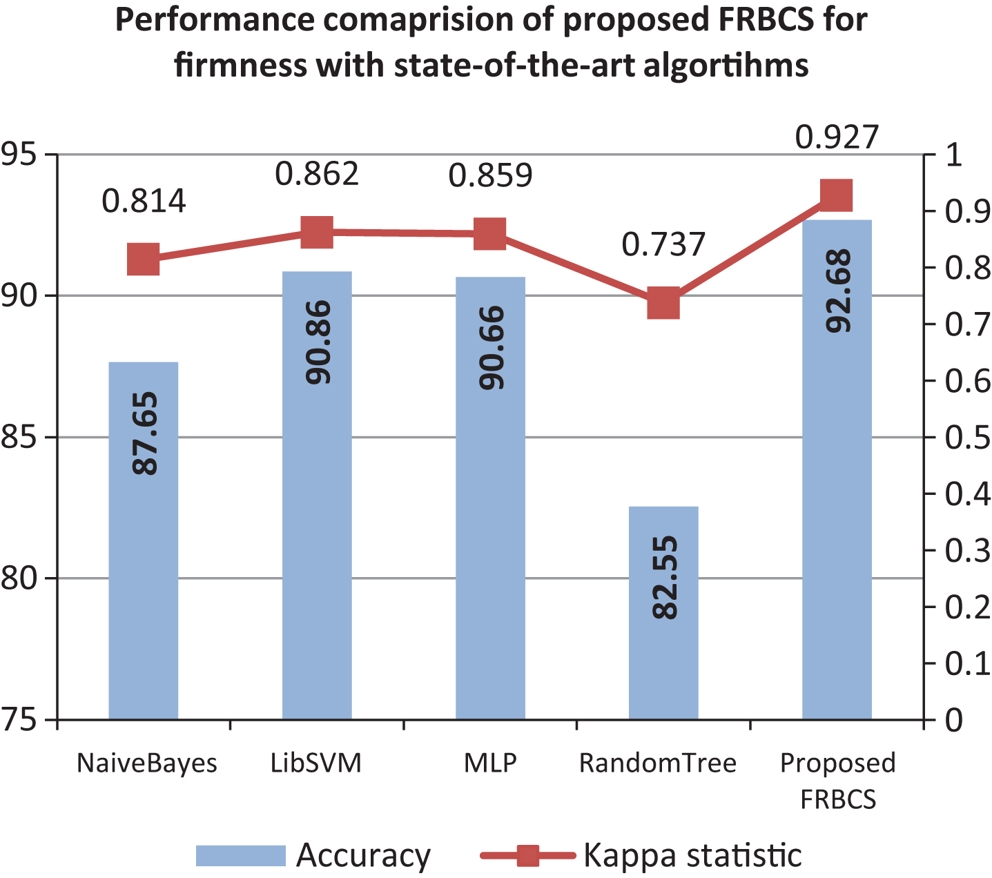
Performance comparison of proposed FRBCS with state-of-art algorithms.

5 Conclusion

The paper presents the two-fold work i.e. non-destructive prediction of firmness using a low cost digital color camera and fuzzy classification of predicted firmness. An empirical analysis of number of different texture analysis methods was carried out for predicting the mechanical property i.e. firmness of tomato. Prediction model was established using RBF regressor, which is a fully supervised approach, based on RBF networks for modeling. Wavelet texture feature showed best statistical performance amongst all the features. Furthermore, based on predicted firmness, proposed FRBCS classifies the tomatoes into three fuzzy classes i.e. soft, medium, and hard. The fuzzy classification aids in improved representation of the consumers’ fuzzy aspect of understanding the firmness. In whole, the system provides the self-sufficient system for estimating and classifying the tomatoes based on the firmness non-destructively and at a very low cost. The proposed approach brings out the viability of using simple imaging system for real-time applications in agriculture.

References

Tijskens

and Evelo

, Modelling colour of tomatoes during postharvest storage, Postharvest Biology and Technology4 (1994), 85–98.

Patel

K.K.

, Kar

, Jha

and Khan

, Machine vision system: A tool for quality inspection of food and agricultural products, Journal of Food Science and Technology49 (2012), 123–141.

Narendra

and Hareesha

, Prospects of computer vision automated grading and sorting systems in agricultural and food products for quality evaluation, International Journal of Computer Applications1 (2010), 1–9.

Borah

, Hines

and Bhuyan

, Wavelet transform based image texture analysis for size estimation applied to the sorting of tea granules, Journal of Food Engineering79 (2007), 629–639.

C.-J.

and Sun

D.-W.

, Learning techniques used in computer vision for food quality evaluation: A review, Journal of Food Engineering72 (2006), 39–55.

García-Ramos

F.J.

, Valero

, Homer

, Ortiz-Cañavate

and Ruiz-Altisent

, Non-destructive fruit firmness sensors: A review, Spanish Journal of Agricultural Research3 (2005), 61–73.

Sirisomboon

, Tanaka

, Kojima

and Williams

, Nondestructive estimation of maturity and textural properties on tomato ‘Momotaro’ by near infrared spectroscopy, Journal of Food Engineering112 (2012), 218–226.

Mollazade

, Omid

, Tab

F.A.

, Kalaj

Y.R.

, Mohtasebi

S.S.

and Zude

, Analysis of texture-based features for predicting mechanical properties of horticultural products by laser light backscattering imaging, Computers and Electronics in Agriculture98 (2013), 34–45.

, Predicting firmness and sugar content of sweet cherries using near-infrared diffuse reflectance spectroscopy, Transactions-American society of Agricultural Engineers44 (2001), 1265–1274.

10.

Nicolai

B.M.

, Beullens

, Bobelyn

, Peirs

, Saeys

, Theron

K.I.

, et al. Nondestructive measurement of fruit and vegetable quality by means of NIR spectroscopy: A review, Postharvest Biology and Technology46 (2007), 99–118.

11.

Qing

, Ji

and Zude

, Predicting soluble solid content and firmness in apple fruit by means of laser light backscattering image analysis, Journal of Food Engineering82 (2007), 58–67.

12.

Qing

, Ji

and Zude

, Non-destructive analyses of apple quality parameters by means of laser-induced light backscattering imaging, Postharvest Biology and Technology48 (2008), 215–222.

13.

Studman

, Computers and electronics in postharvest technology—a review, Computers and Electronics in Agriculture30 (2001), 109–124.

14.

Qiao

, Wang

, Ngadi

and Kazemi

, Predicting mechanical properties of fried chicken nuggets using image processing and neural network techniques, Journal of Food Engineering79 (2007), 1065–1070.

15.

Karimi

, Fathi

, Sheykholeslam

, Sahraiyan

and Naghipoor

, Effect of different processing parameters on quality factors and image texture features of bread, J Bioprocess Biotech2 (2012), 2.

16.

Sehgal

and Goel

, Auto-annotation of tomato images based on ripeness and firmness classification for multimodal retrieval, in International Symposium on Advances in Applied Informatics (SAI’16), India, 2016.

17.

Sirisomboon

, Tanaka

and Kojima

, Evaluation of tomato textural mechanical properties, Journal of Food Engineering111 (2012), 618–624.

18.

Vursavus

K.K.

, Yurtlu

Y.B.

, Diezma-iglesias

, Lleo-garcia

and Ruiz-altisent

, Classification of the firmness of peaches by sensor fusion, Int J Agric & Biol Eng8 (2015), 104–115.

19.

Chherawala

, Lepage

and Doyon

, Food grading/sorting based on color appearance trough machine vision: The case of fresh cranberries, in Information and Communication Technologies, 2006 ICTTA’06 2nd, 2006, pp. 1540–1545.

20.

Zhang

, Yin

, Xu

and Zhao

, On-Line Sorting Maturity of Cherry Tomato Bymachine Vision, in Computer and Computing Technologies in Agriculture II, Volume 3, ed: Springer, 2009, pp. 2223–2229.

21.

Bulanon

, Kataoka

, Okamoto

and Hata

, Development of a real-time machine vision system for the apple harvesting robot, in SICE 2004 Annual Conference, 2004, pp. 595–598.

22.

Wang

, Zhu

and Ji

, Machine vision based cotton recognition for cotton harvesting robot, in Computer And Computing Technologies In Agriculture, Volume II, ed: Springer, 2008, pp. 1421–1425.

23.

Xiao-Lian

, Xiao-Rong

and Bing-Fu

, Identification and Location of Picking Tomatoes Based on Machine Vision, in Intelligent Computation Technology and Automation (ICICTA), 2011 International Conference on, 2011, pp. 101–107.

24.

Zou

and Zhao

, Machine Vision Online Measurements, in Nondestructive Measurement in Food and Agro-Products, ed: Springer, 2015, pp. 11–56.

25.

Wang

, Huang

and Zhu

, Model fusion for prediction of apple firmness using hyperspectral scattering image, Computers and Electronics in Agriculture80 (2012), 1–7.

26.

Goel

and Sehgal

, Adaptive segmentation technique for recognizing tomatoes at different maturity stages, in International Conference on Computer, Control, Informatics and its Applications (IC3INA 2014), Indonesia, 2014.

27.

Haralick

R.M.

, Statistical and structural approaches to texture, Proceedings of the IEEE67 (1979), 786–804.

28.

Zheng

, Sun

D.-W.

and Zheng

, Recent applications of image texture for evaluation of food qualities—a review, Trends in Food Science & Technology17 (2006), 113–128.

29.

Tang

, Texture information in run-length matrices, Image Processing, IEEE Transactions on7 (1998), 1602–1609.

30.

Mallat

, A wavelet tour of signal processing: Academic Press, 1999.

31.

Antonini

, Barlaud

, Mathieu

and Daubechies

, Image coding using wavelet transform, Image Processing, IEEE Transactions on1 (1992), 205–220.

32.

Goel

and Sehgal

, Fuzzy classification of pre-harvest tomatoes for ripeness estimation–An approach based on automatic rule learning using decision tree, Applied Soft Computing36 (2015), 45–56.

33.

Witten

I.H.

, Frank

and Mark

, “Hall (2011) ” Data Mining: Practical machine learning tools and techniques,” ed: Morgan Kaufmann, San Francisco. Retrieved, 2011.

Total number of instances	133
Accuracy	92.68%
Incorrectly classified Instances (in %)	7.31%
Kappa statistics	0.9265

Non-destructive low-cost approach for fuzzy classification of tomato images based on firmness prediction using regression

Abstract

Keywords

1 Introduction

2 Material and methods

2.1 Data set

2.2 Objective/instrumental texture evaluation

2.4 Image texture analysis

2.4.1 First order statistics (FOS)

2.4.3 Gray level run length matrix (GLRLM)

2.4.4 Wavelet transform

2.6 Prediction model

4.1 Firmness prediction

Table 11 Evaluation metrics for the proposed FRBCS Total number of instances 133 Accuracy 92.68% Incorrectly classified Instances (in %) 7.31% Kappa statistics 0.9265

References

Table 11
Evaluation metrics for the proposed FRBCS

Total number of instances 133

Accuracy 92.68%

Incorrectly classified Instances (in %) 7.31%

Kappa statistics 0.9265