Connected components labeling based on union-find operations applied to connected branches

Abstract

This paper presents an efficient run-based algorithm for labeling connected components in a binary image. By means of two tables called index table and equivalent information table respectively, the algorithm assign labels only to run sets which are composed of a series of runs connected to each other in adjacent scan rows, then the same index in equivalent information table can be assigned to all runs of a set in index table at one time. Further, the algorithm organizes all equivalence information in equivalent information table in a tree structure, and employee the union-find technique to merge connected components rapidly. The algorithm is very simple, and fewer operations are needed to check and to label runs of a connected branch. Furthermore, it is not necessary to calculate the minimum label while combining two runs, and is able to construct a union-find tree with smaller height. Thus the algorithm is able to provide a high speed to label connected components for general images.

Keywords

Connected components union-find labeling algorithm label equivalent run length encoding

1 Introduction

Connected component labeling (CCL) is a procedure for detecting all the object pixels of the same connected component in a binary image, or for assigning a unique label to every connected component. Since the number and features of connected components are keys for other analytical procedures, connected component labeling plays a very important role in computer vision, pattern recognition, medical image processing, image compression and other fields. Therefore, many researches have been done for addressing this issue [1 –4]. There are a number of different approaches to labeling connected components, and we can briefly summarize these methods into two categories: one depending on the hardware structure and the other applying to the general computer architecture. The first category includes hardware-based parallel algorithms [5], run-based algorithms depending on GPU and shared memory [6, 7], algorithms aimed on hardware acceleration and less memory occupation [8], block-based algorithms depending on new architecture and cache memory, and those based on FPGA [9 –13]. In the second category, the most widely used algorithms for general architecture and pixel representation can be grouped into multi-pass algorithms, two-pass algorithms and one-pass algorithms.

Multi-pass algorithms [14]. These algorithms scan an image and update labels of pixels of connected components repeatedly until no pixel label changed. The number of passes depends on the geometrical complexity of connected components. Generally, they are simple but with lower efficiency.

Two-pass algorithms [15 –30]. These algorithms operate in three distinct phases. In the first phase, the image is scanned once to assign provisional labels to object pixels, and to record the equivalence information among provisional labels. In the second phase, they analyze the label equivalence information to determine the final labels. In the end they assign a unique representative label to every object pixel.

One-pass algorithms [31 –38]. Contour tracing and seed-growth method are the typical representatives. In contour tracing algorithms, they search an unlabeled border pixel of a connected component first and assign a new label to it. Then they trace the whole border of the components, and mark all pixels in the border with the same labels. Such processing is executed iteratively until there is no unlabeled pixel in the image. In seed-growth algorithms, they label an unlabeled inner pixel of a component first, and expand the scope of pixels gradually by labeling its neighbors until all pixels of the components are labeled.

Besides, there exist some algorithms dealing the problem to label connected components in 3D images [27, 30]. A special algorithm which scans image lines every three lines and processes pixels three by three is proposed in [39].

In this paper, we propose a novel run-based two-scan labeling algorithm for binary image. In the algorithm, all runs are assigned changeless indexes of location in the equivalence information (label) table. By this operation a series of runs connected to each other in adjacent scan rows are aggregated into a whole set naturally before they are merged into a bigger connected component. We assign a unique label to each set of runs, and then apply the equivalence information processing only to run set rather than runs or pixels. At the same time, the Union-Find technique is employed to merge equivalent information. Since the number of run set is far less than that of runs or pixels, and fewer nodes are visited while sets are merged, our algorithm can complete the connected components labeling efficiently.

The rest of this paper is organized as follows: we review several typical labeling algorithms in the next section. We introduce our algorithm in Section 3. In Sections 4 and 5, we show our experimental results and analyze the efficiency of the algorithms. We give our conclusion in the Section 6.

2 Connectivity analysis

For a W×H binary image, where H and W are numbers of rows and columns respectively, we use a 2-D array p(x, y) or a 1-D array p(y×W +x) to denote the pixel value at (x, y), where 0 ≤ x < W and 0 ≤ y < H, and I_f for the pixel value of the object pixel and I_b for that of the background pixel. The goal of connected components labeling is to assign a label L(x, y) to each foreground pixel and assign a unique label to a set of connected object pixels in a binary image which is called a connected component.

Connectivity between pixels commonly can be divided into two cases such as 4-connected and 8-connected, and only 8-connected components is considered in these paper. Figure 1 shows a foreground pixel p and its 8-neighberhood mask (3×3 mask) M_S. When a neighbor pixel q belonging to the spatial support of M_S is foreground pixel, it is 8-connected to pixel p, and they should be assigned to same label.

Fig.1

8-neighberhood mask M S of the pixel p under analysis is composed of 8 pixels except p.

A run is a block of contiguous object pixels in a row. A run from p(s) to p(e) in an image is described by r(s,e) when the image is stored in a 1-D array. If the current run r(s,e) in the scan row is 8-connected to a run r(u,v) in above row, we can check this with a simple criterion where, $(s \leq v + 1) \land (e \geq u - 1)$ (1)

By 8-connected connectivity we know that all pixels of run r(s,e) and run r(u,v) belong to one connected components, as shown in Fig. 2.

Fig.2

Three runs are 8-connected to run r(12,17), thus all pixels of them belong to one connected components.

For a W × H binary image, we know that the maximum of run number is ⌈W/2 ⌉ × H, and the maximum of connected components (i.e. labels) number is also ⌈W/2⌉ × ⌈ H/2 ⌉.

A downwards connected branch (DCB) is defined as a run set which is composed of a start run and all subsequent runs connected to it in adjacent scan rows, and all runs occupy one position index in equivalence table collectively, as shown in Fig. 3. It is obvious that there are more pixels in a DCB than that in a run. Soon afterwards we will explain how to speed up the connected component labeling algorithm by means of DCB.

Fig.3

A DCB composed of nine runs (Starting from the run r_start).

3 Proposed algorithm

3.1 Outline

For a W × H binary image described in pixels pattern such as BMP, all pixel values are stored in a 1-D array p (y × W + x) in our algorithm, where 0 ≤ x < W and 0 ≤ y < H. We use an equivalence information table Label to store all labels of DCBs explained in Section 2.1, and a table Index, called index table, to store every label index of run in Label. In other words, the label of DCB which the ith run belongs to is stored in element Label[Index[i]].

Our algorithm scans every pixel in the input image and implements connected components labeling in this way:

Firstly, we scan pixel p(i) one by one in the current row to find out and record all runs. Each run is processed to test its connectivity with all runs above the scan row in the raster scan direction. There are three different cases for the label assignment problem:

When there are no runs above the scan row is connected with the current run, we will add a new label to the table Label, and set this index to the label index of the current run in Index. In fact, this index is the label of DCB starting from the current run or points to the position in Label to store its link relation.

If there is only one run r(s,e) in above row connected with the current run, this means that the current run belongs to the DCB which r(s,e) belongs to. Thus we only assign the index of r(s,e) to the current run.

When there is more than one run in above row connected with the current row, denoted by r(s_i,e_i), where 1 ≤ i ≤ m, we will merge all components including r(s_i,e_i) (2≤i≤m) to the components which r(s₁,e₁) belongs to by means of the Union-Find technique according to the indexes of all r(s_i,e_i). Moreover, we assign the index of r(s₁,e₁) to the current run. This means that the current run belongs to the DCB which r(s₁,e₁) belongs to. After this, our algorithm returns to scan next row until all rows in the image are handled.

Secondly, we scan the table Label to update all equivalence provisional labels (items in a path) with representative labels. At the last we fill all pixels in the image with labels gained from the table Label.

For an instance, Fig. 4(a) shows the status after all rows in the first three rows have been processed, and Fig. 4(b) illustrates the handling method for the rows in the 4th row.

Fig.4

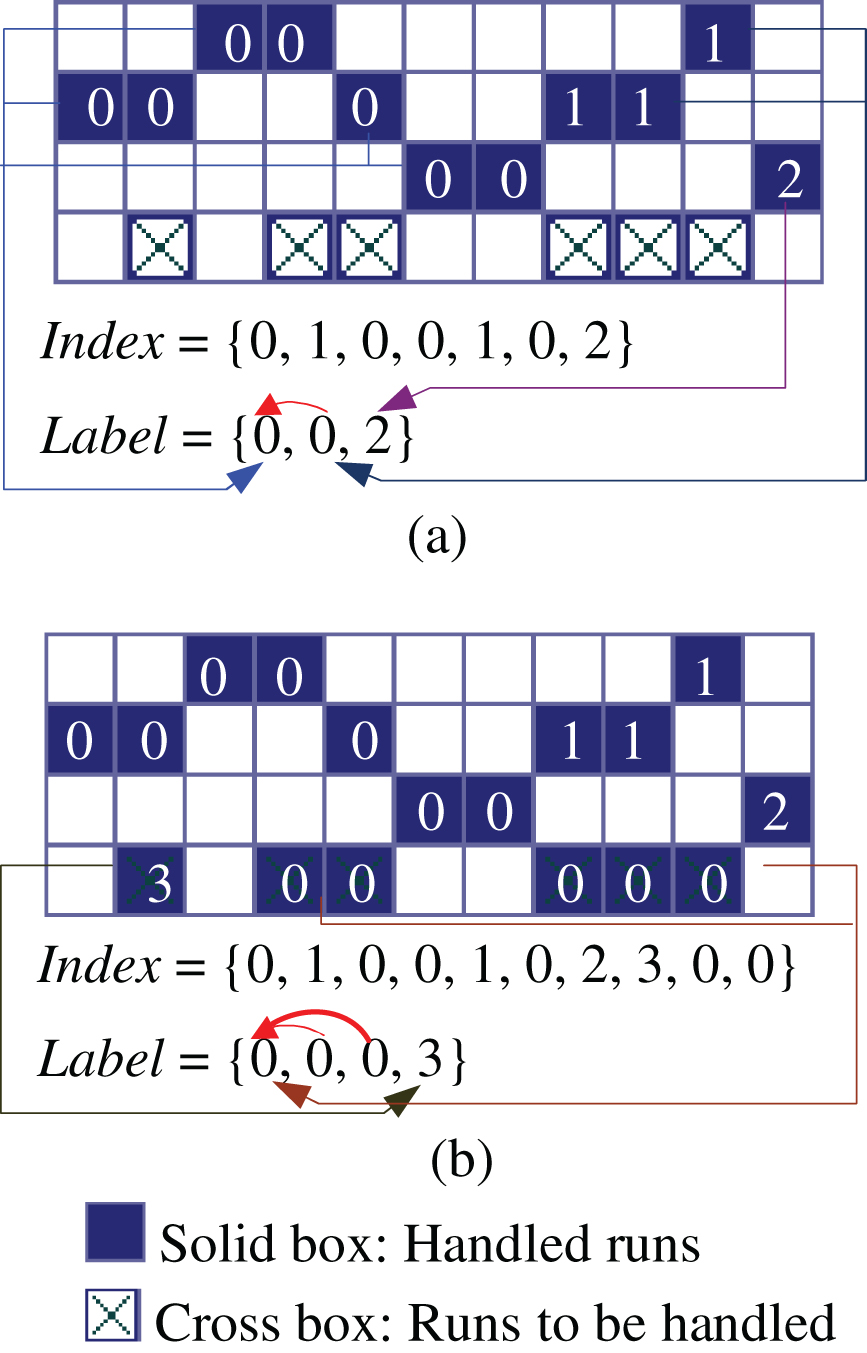
Handling the runs in the 4th row: creating a new DCB, adding a run to a DCB and merging two components.

Different from conventional algorithms, when a new run is found out, it is assigned an index of DCB which it belongs to in the table Label rather than a provisional label. This separates equivalence information from run data. All runs of one DCB keep only one index which will never need to be changed, and occupy one item in the table Label. When two runs are connected with each other in step iii), only two sets of the indexes of DCBs to which they belong are merged. Since the table Label is composed of the labels associated with DCBs rather than runs, its size is far smaller than number of runs. With the addition of near linear time complexity of a Union-Find procedure applied to the table Label, computation can be greatly reduced.

3.2 Implementation

In consideration of the number of runs and labels in a W × H binary image p, we use a ⌈W/2 ⌉ × H-size 1-D array Index to store label indexes of runs, and a ⌈W/2⌉ × ⌈ H/2 ⌉-size 1-D array Label to store and handle the equivalence information. During the first scan, each Index[i] represents an index of representative label of a DCB which the ith run belongs to in the table Label.

Let us define some notations:

p The pointer of image data

c The number of runs with the initial value of zero

l The next label to be assigned with the initial value of zero

s The array of starting positions of runs

e The array of end positions of runs

cc The number of connected components

While we search runs in a scan row, for avoiding testing end of the row, we expand the width of the image W to W + 1, and fill all pixels in the last column with background color.

The labeling procedure follows the below steps in our algorithm:

1:	c = 0, l = 1, u = 0;
2:	size = W*H;
3:	for(i = 1; i < size; i++){
4:	if(p) {
5:	s[c] = i;
6:	i++;
7:	while(p[i]) i++;
8:	e[c] = i-1;
9:	while(e[u] < s[c]-W-1) u++;
10:	if(e[u]≤e[c]-W) {
11:	Index[c] = Index[u];
12:	f = u;
13:	u++;
14:	while(e[u]≤e[c]-W) {
15:	Union(Label, Index[f], Index[u]);
16:	u++;
17:	}
18:	if(s≤e[c]-W+1)
19:	Union(Label, Index[f], Index[u]);
20:	}
21:	else {
22:	if(s[u]≤e[c]-W+1)
23:	Index[c] = Index[u];
24:	else {
25:	Index[c] = l;
26:	Label[l] = l;
27:	l++;
28:	}
29:	}
30:	c++;
31:	}
32:	}
33:	cc = 0;
34:	for(i = 1; i < l; ++i) {
35:	if(Label[i] ≠ i)
36:	Label[i] = Label[Find(Label, Label[i])];
37:	else++cc;
38:	}

The structure of the first section in the algorithm before Line 32 is similar to that in literature [38], but there exist some differences. We scan pixel p[i] one by one for the given image p (Line 3), and starting position and end position of a new found run are recorded by s[c] and e[c] respectively (from Line 4 to Line 8).

For the current run r(s[c], e[c]), we pass all recorded runs in the above row which are not connected to r(s[c], e[c]), and locate the first recorded run r(s[u], e[u]) which is possible connected to r(s[c], e[c]) (Line 9). After this, we check whether r(s[u], e[u]) ends before r(s[c], e[c]) (Line 10). If it does, we assign r(s[c], e[c]) the same index of the run in the table index (Line 11), and this makes r(s[c], e[c]) to be added into the current DCB. This run is the first run connected to r(s[c], e[c]), and we record it with f (Line 12). Furthermore, for each other consecutive recorded run r(s[u], e[u]) connected to r(s[c], e[c]), we merge the equivalent information set S(Label[Index[u]]) which the element Label[Index[u]] belongs to and the first set S(Label[Index[f]]) which the element Label[Index[f]] belongs to (from Line 14 to Line 16). Since the run start before/at e[c]-W+1 is connected to r(s[c], e[c]), we merge the set S(Label[Index[u]]) which it belongs to and the first set S(Label[Index[f]]) (from Line 14 to Line 16). Otherwise, if r(s[u], e[u]) ends after r(s[c], e[c]), we add r(s[c], e[c]) into the equivalent information set S(Label[Index[u]]) which the element Label[Index[u]] belongs to by assigning r(s[c], e[c]) the index of r(s[u], e[u]) (from Line 22 to Line 23). Otherwise r(s[c], e[c]) is not connected to any recorded DCB, or say, it represents a new DCB, thus we assign it a new index l in the table Index, and set provisional label l to itself (Line 25 and Line 26). Further, we increase l by 1 for provisionally labeling the next run which is not connected to any recorded run.

After handling the current run, we increase n by 1 for recording and handling the next run (Line 30).

After the end of the scan, l is the actual length of the table Label, or to say the number of DCBs, and c is the number of runs. Since all trees composed of DCBs are stored in table Label, for obtaining connected components, we need to scan the table Label once to replace all provisional labels with representative labels recorded in their roots of trees. In this process, for each node Label[i], we employ the function Find to locate the root of the tree which it belongs to (from Line 34 to Line 35). Then we assign it the index of the root of the tree (Line 36). After this, for the ith run in the table Index, Label[Index[i]] is the representative label assigned to the connected component it belongs to. Besides, the procedure accumulates the number of elements meeting the condition Label[i] = i to gain cc (Line 37), the number of connectedcomponents.

After this, all runs that belong to a connected component will have the same representative label. Thus we can assign the representative label corresponding to a run to all its object pixels directly where,

for(i = 0; i < c; ++i) {

t = Label];

for(x = s[i]; x≤e[i]; ++x) p[x] = t;

}

3.3 Merging sets by the union-find technique

In this section we will briefly discuss about how to implement union and find operations on the equivalence information table Label.

In our algorithm, each element of the table Label represents a representative label or an index of its parent, rather than all representative labels. as discussed earlier, for each scan, every time a run not connected with any runs above the scan row is found, a new element will be added to the table Label with operation Label[l] = l, where l is a new label assigned to the DCB which represents the root of the connected component. Thus the condition Label[l] = l can be used to find the root node of a tree. Besides, if a node v needs to be linked to a tree with the root node u, we should implement the operation as follows: $Label [v] \leftarrow u$

Algorithm 1 shows the description of the function Find. It locates the root node of tree of the node pos by a recursive procedure. In function Find, the variable pos takes on a path from the starting node pos to the root of the tree called find path. For reducing the depth of the tree, the function changes all nodes on the find path to point directly to the specified new root in each iteration processing.

Algorithm 1 long Find(Label, pos)

{

if(Label ≠ pos) {

Label[pos] = Find (Label, Label[pos]);

returnLabel[pos];

}

returnpos;

}

Different from common algorithms, our function Union shown in algorithm 2 merges all connected components into the leftmost component directly rather than into the minimum label one, and return the root of the merged tree. This makes comparison operations between labels and update operation for all items in a set which is merged to be omitted. The successful test to x = y demonstrates that they belong to the same components and needed not to bemerged.

Algorithm 2 long UnionA(Label, pos1, pos2)

{

x = Find(Label, pos1);

y = Find(Label, pos2);

if(x = y) returnx;

Label = x;

returnx;

}

In most instances, there is no need to keep the depth of the union-find tree as short as possible. On the contrary, the path update leads tree nodes to be visited again and again while it is merged into others repeatedly. When a node v should be combined with a node u, we need only to link the tree to which the node v belongs to the node u. Thus we update the algorithm with a new version as shown inAlgorithm 3.

Algorithm 3 void Union (Label, pos1, pos2)

{

if(Label = Label[pos2])

return;

while(Label[pos2] ≠ pos2) {

t = Label[pos2];

Label[pos2] = Label[pos1];

pos2 = t;

}

Label[pos2] = Label[pos1];

}

This procedure can link the root of the tree including the node pos2 to the node pos1 rather than its root, and only the find path of the former is reduced. We can see that the algorithm runs faster by replacing the first version with the second one.

4 Experimental results

Our computer implementations were developed using the C++ language and the C++ Builder 6.0 compiler. The desktop computer for the tests is an Intel Pentium Dual-Core CPU E5300 with a processor running at 2.60 GHz and 4 GB RAM memory (Windows XP OS). All data in this section were obtained by averaging of the execution time for 5000 runs.

We mainly compared our algorithm with the following newest representative labeling algorithms: the Scan plus Array-based Union-Find (SAUF) labeling algorithm proposed in [24], the Optimized Block-Based (BBDT) labeling algorithm proposed in [25], the Contour-Tracing labeling (CT) algorithm proposed in [33], and the optimized Run-based Two-Scan (or to say, One-and-a-Half-Scan) algorithm (RBOH) proposed in [37]. The programs of the SAUF algorithm and the CT algorithm were provided by their authors.

The image format was used for the tests is BMP (Bitmap), and the total execution time for whole labeling procedure was used for comparison from run detecting, connectivity checking to run label assigning, and at last every pixel is assigned a representative label in the image. Two kinds of images were tested in this section:

(1) The first test set is downloaded from the Standard Image Databases of the University of Southern California including miscellaneous Database, textures Database and aerials Database. They are composed of 20, 12 and 30 images respectively. All of these images 512 × 512 in size, and were transformed into binary images by means of Otsu’s threshold selection method. The comparison results are listed in Table 1.

Table 1
Comparison of various execution times [msec] on various kinds of images

Image Type Item #CC Execution time (ms)

SAUF CT RBOH BBDT Ours

Miscellaneous Max. 3027 8.95 7.80 2.66 5.46 2.57

mean 1019 6.05 5.03 1.58 3.57 1.52

Min. 65 3.29 3.63 0.92 2.57 0.85

Aerials Max. 4091 11.11 8.05 2.81 6.44 2.71

mean 1605 7.69 6.05 2.08 4.90 2.02

Min. 413 6.87 4.97 1.74 4.05 1.69

Textures Max. 4498 10.19 11.39 4.31 8.65 4.25

mean 1705 7.38 7.78 2.75 5.35 2.67

Min. 106 2.89 3.46 0.79 2.59 0.76

Image Type	Item	#CC	Execution time (ms)
Miscellaneous	Max.	3027	8.95	7.80	2.66	5.46	2.57
	mean	1019	6.05	5.03	1.58	3.57	1.52
	Min.	65	3.29	3.63	0.92	2.57	0.85
Aerials	Max.	4091	11.11	8.05	2.81	6.44	2.71
	mean	1605	7.69	6.05	2.08	4.90	2.02
	Min.	413	6.87	4.97	1.74	4.05	1.69
Textures	Max.	4498	10.19	11.39	4.31	8.65	4.25
	mean	1705	7.38	7.78	2.75	5.35	2.67
	Min.	106	2.89	3.46	0.79	2.59	0.76

#CC, number of connected components.

The results for six representative images are illustrated in Fig. 5, where the object pixels are displayed in black.

Fig.5

Results for six representative images.

(2) The second test set is composed of images with some structured patterns on them. The four kinds of elementary patterns of these images, called finger, step, spiral, zigzag, keys and chain are shown in Fig. 6 (a)∼(f) respectively.

Fig.6

Six elementary patterns to construct benchmark images.

The test results for these benchmark images constructed using the elementary patterns withvarying image sizes are shown in Fig. 7, Tables 2and 3.

Fig.7

Comparison of the performance of several algorithms when different patterns are used as input images.

Table 2

Comparison of various execution times [msec] on various kinds of images width size =4086 × 4086

Algo.	Finger	Step	Spiral	Zigzag	Keys	Chain
SAUF	620	750	534	422	882	534
CT	705	965	914	708	631	853
BBDT	359	666	475	432	530	477
RBOH	247	183	244	246	243	319
OURS	223	179	227	225	219	289

Table 3

Comparison of various execution times [msec] on various kinds of images width size = 512×512

Algo.	Finger	Step	Spiral	Zigzag	Keys	Chain
SAUF	9.51	10.58	8.12	6.46	13.67	8.13
CT	10.89	14.21	14.40	10.92	9.62	13.07
BBDT	5.77	9.09	7.34	6.66	7.88	7.31
RBOH	3.72	2.81	3.74	3.61	3.74	4.64
OURS	3.42	2.77	3.57	3.34	3.38	4.46

5 Analysis and comparison

As we can see, for general images, our algorithm can increase speed of operations to label connected component in different degrees, and is only a small dip in geometric complexity of the components in images.

i) Comparison with SAUF algorithm and BBDT algorithm. SAUF algorithm is pixel-based. By means of speeding up the test technique for pixel connectivity with decision-tree, the time needed for testing connectivity among pixels in the spatial support of M_S is reduced. This technique is more effective for dealing with the local pattern with complex structure and short runs. Thus SAUF algorithm may show good performance for labeling the images such as noisy images. Since all pixels need to be assigned provisional labels, the number of operations consumed on each pixel averagely is more than that in run-based algorithm. Furthermore, the union-find operation needs to be applied to all pixels in SAUF algorithm to guarantee that the algorithm can join them to root node of a tree correctly. BBDT algorithm speeds up the work by optimal decision tree and new scan method depending on 2×2 pixel grid efficiently, but it also treats the image in the same way as SAUF. In our algorithm, only once assignment operation is needed to handle every run (i.e. all pixels) of a DCB except its first run. Each DCB occupies only one item in the table Label which denotes the shared label of all runs in the DCB, thus the height of label tree (or forest) is much smaller than that in SAUF algorithm. This makes our algorithm to implement union-find operation in a lower time complexity.

ii) Comparison with RBOH algorithm. Roughly speaking, RBOH algorithm is a run-based version of RTS algorithm in [20] (including [26] and [27]), and works faster than RTS algorithm. We think that it is the fastest run-based algorithm among proposed ones. At the point to as far as possible to reduce the time consuming to handle runs in a DCB, our algorithm is similar to RBOH algorithm. However, when several connected components should be merged, RBOH algorithm needs to find out the minimum one of their provisional labels, and all provisional labels in components which should be merged must be modified with the minimum label. For those images with small runs and complicated structure, this kind of operation will be invoked frequently, and items of label set will be visited repeatedly. This can be shown in Fig. 8, and the variations of equivalence information tables while algorithms scan the image are shown in Table 4.

Fig.8

A test image like keys of a piano.

Table 4

Variations of equivalence information tables

Row	r_label in RBOH							Label in OURS
1	1	2	3	4	5	6	7	0	1	2	3	4	5	6
2	1	2	3	4	4	4	4	0	1	2	3	3	3	3
3	1	2	3	3	3	3	3	0	1	2	2	3	3	3
4	1	2	2	2	2	2	2	0	1	1	2	3	3	3
5	1	1	1	1	1	1	1	0	0	1	2	3	3	3

Notes: The gray boxes demonstrate all items which are modified as scanning the image.

Our algorithm does not require the calculation for the minimum provisional label. The main differences between our algorithm and RBOH algorithm (including RTS algorithm) is, when two label sets of equivalence information S₁ and S₂ should be merged, RBOH algorithm needs to visit all items of S₁ (or S₂) to modify their values. By comparison, only partial items of S₁ and S₂ are visited since they are organized with tree structure rather than list structure in our algorithm. This can speed up merging efficiency for the case that the sizes of S₁ or S₂ are large. In other words, the multiple visits to all items are replaced by once correction-scan for the table Label at the last. Experiments show that our algorithm is about 5% ∼10% faster than RBOH algorithm.

iii) Comparison with CT algorithm. Firstly, our algorithm is much faster than the CT algorithm for all images used in our test set. Secondly, our algorithm handles an image in the raster scan order rather than an irregular way used by the CT algorithm. This makes it to be suitable for hardware implementation and parallel implementation. However, after labeling the CT algorithm can extract contours of connected components, where are also important for some image processing application.

In order to record provisional labels assigned to pixels, conventional two-pass algorithm, SAUF algorithm and CT algorithm modify pixels of input image directly. Thus, these algorithms need to use an integer (16-bit or 32-bit in C++) array to store input image. In addition a table with size M × N/4 is used to handle representative labels. In run-based algorithms, including RTS algorithm, RBOH algorithm and our algorithm, it does not modify original image directly, and use two tables with size M × N/2 to store run information. Thus the input binary image can be described by means of a bit array. Besides, our algorithm employees a table Index with size M × N/2 to record indexes of runs, and a table Label with size M × N/4 to handle representative labels. Similar method is also adopted by RBOH algorithm, but three tables are used to handle representative labels. Thus our algorithm consumes lower memory than that of RBOH algorithm and little more than that of the SAUF algorithm, BBDT algorithm and the CT algorithm.

Generally, representative labels assigned with our algorithm is not consecutive. If we prefer consecutive labels, we only need to sort the representative labels table Label before assigning labels to all pixels where,

j = 1;

for(i = 0; i < l; i++)

if(Label = i) Label[i] = j++;

Since l is very smaller than the number of runs, this process takes very little time. This procedure is the same as that used for general Union-Find set [4].

6 Conclusion remarks

In this paper, we present a fast run-based two-scan algorithm for labeling connected components in a binary image. The algorithm maps all labels of runs in a DCB into one item of the label table, and stores all equivalence information in a tree structure. Thus the algorithm is able to handle equivalence information on a connected branch set rather than a run set. Furthermore, by means of developed union-find procedure, the algorithm finds out all connected components on a smaller data set and merges them rapidly. Thus the algorithm has the advantages of easy implementation and less time consumption.

For future work, we plan to develop our algorithm to label 3-D connected components.

References

Rosenfeld

, Connectivity in digital pictures, Journal of the ACM17(1) (1970), 146–160.

Hecquard

and Acharya

, Connected component labeling with linear octree, Pattern Recognition24(6) (1991), 515–531.

Dillencourt

, Samet

and Tamminen

, General approach to connected-component labeling for arbitrary image representations, Journal of the ACM39(2) (1992), 253–280.

Fiorio

and Gustedt

, Two linear time union-find strategies for image processing, Theoretical Computer Science154(2) (1996), 165–181.

Flatt

, Blume

, Hesselbarth

, et al., A parallel hardware architecture for connected component labeling based on fast label merging, Proceeding of Application-Specific Systems, Architectures and Processors (2008), 144–149.

Chen

, Zhao

H.L.

, Tao

, et al., Block-run-based connected component labelling algorithm for GPGPU using shared memory, Electronics Letters47(24) (2011), 1309–1311.

Jung

and Jeong

, Parallel connected-component labeling algorithm for GPGPU applications, Communications and Information Technologies (ISCIT) (2010), 1149–1153.

Zhao

, Zhang

, et al., A hardware acceleration based algorithm for real-time binary image connected-component labelling, J Electronics & Information Technology33(5) (2011), 1069–1075.

Ito

and Nakano

, Low-latency connected component labeling using an FPGA, International Journal of Foundations of Computer Science21(3) (2010), 405–425.

10.

Ito

, Nakano

, and

and Pan

, Optimized component labeling algorithm for using in medium sized FPGAs, Proceedings of Ninth International Conference on Parallel and Distributed Computing, Applications and Technologies (2008), 171–176.

11.

Grana

, Borghesani

and Cucchiara

, Connected component labeling techniques on modern architectures, Lecture Notes in Computer Science5716 (2009), 816–824.

12.

Lee

, Jin

, Thien

, et al., FPGA based connected component labeling, Proceedings of International Conference on Control, Automation and Systems (2007), 2313–2317.

13.

Calvo-Gallego

, Cabrera

A.A.

, Brox

, et al., Real-time FPGA connected component labeling system, Proceedings of 19th IEEE International Conference on Electronics, Circuits and Systems (2012), 593–596.

14.

Suzuki

, Horiba

and Sugie

, Linear-time connected-component labeling based on sequential local operations, Computer Vision and Image Understanding89(1) (2003), 1–23.

15.

Wang

, Luo

, Wang

, et al., New algorithm for binary connected-component labeling based on run-length encoding and union-find sets, Journal of Beijing Institute of Technology19(1) (2010), 71–75.

16.

Lacassagne

and Zavidovique

, Light speed labeling: Efficient connected component labeling on RISC architectures, J Real-Time Image Processing6(2) (2011), 117–135.

17.

De Bock

and Philips

, Fast and memory efficient 2-D connected components using linked lists of line Segments, IEEE Transactions on Image Processing19(12) (2010), 3222–3231.

18.

Sutheebanjard

and Premchaiswadi

, Efficient scan mask techniques for connected components labeling algorithm, Proceedings of EURASIP J on Image and Video Processing (2011), 14–20.

19.

Yeong

, Ang

and Seng

, Efficient connected component labeling using multiple-bank memory storage, Proceedings of 3rd IEEE International Conference on Computer Science and Information Technology (2010), 75–79.

20.

, Chao

and Suzuki

, A run-based two-scan labeling algorithm, IEEE Transactions on Image Processing17(5) (2008), 749–756.

21.

, Chao

and Suzuki

, A new first-scan method for two-scan labeling algorithms, IEICE Transactions on Information and SystemsE95D(8) (2012), 2142–2145.

22.

, Chao

, Suzuki

, et al., A high-speed run-based two-scan labeling algorithm, J the Institute of Image Information and Television Engineers62(9) (2008), 1461–1465.

23.

, Chao

and Ieee, A linear-time two-scan labeling algorithm, IEEE International Conference on Image Processing5(5) (2007), 241–244.

24.

, Otoo

and Suzuki

, Optimizing two-pass connected-component labeling algorithms, Pattern Analysis and Applications12(2) (2009), 117–135.

25.

Grana

, Borghesani

and Cucchiara

, Optimized block-based connected components labeling with decision trees, IEEE Transactions on Image Processing19(6) (2010), 1596–1609.

26.

, Chao

and Suzuki

, Two efficient label-equivalence-based connected-component labeling algorithms for 3-D binary images, IEEE Transactions on Image Processing20(8) (2011), 2122–2134.

27.

, Chao

, Suzuki

, et al., Fast connected-component labeling [J], Pattern Recognition42(9) (2009), 1977–1987.

28.

Paralic

, Fast connected component labeling in binary images, Proceedings of the 35th International Conference on Telecommunications and Signal Processing131(5) (2012), 706–709.

29.

, Qian

and Nowinski

, Fast connected-component labelling in three-dimensional binary images based on iterative recursion, Computer Vision and Image Understanding99(3) (2005), 414–434.

30.

Chang

, Sinica

and Chen

, A component-labeling algorithm using contour tracing technique, Computer Vision & Image Understanding93(2) (2003), 206–220.

31.

Yapa

and Koichi

, A connected component labeling algorithm for grayscale images and application of the algorithm on mammograms, Proceedings of the ACM Symposium on Applied Computing (2007), 146–152.

32.

, Takaki

and Ishii

, A fast multi-object extraction algorithm based on cell-based connected components labelling, IEICE Transactions on Information and SystemsE95D(2) (2012), 636–645.

33.

Chang

, Chen

and Lu

, A linear-time component-labeling algorithm using contour tracing technique, Computer Vision and Image Understanding93(2) (2004), 206–220.

34.

Bai

, Zhang

, Hai

, et al., A new linear-time component-labeling algorithm, Proceedings of the 2nd International Conference on Software Technology and Engineering (2010), 1150–1153.

35.

Abubaker

, Qahwaji

, Ipson

, et al., One scan connected component labeling technique, Proceedings of IEEE International Conference on Signal Processing and Communications (2007), 1283–1286.

36.

, Chao

and Itoh

, A run-based one-scan labeling algorithm, Lecture Notes in Computer Science5627 (2009), 93–102.

37.

, Chao

and Suzuki

, A run-based one-and-a-half-scan connected-component labeling algorithm, International Journal of Pattern Recognition and artificial Intelligence24(4) (2010), 557–579.

38.

Alstrup

, Ben-Amram

and Rauhe

, Worst-case and amortised optimality in Union-Find, Proceedings of the thirty-first annual ACM Symposium on Theory of Computing (1999), 499–506.

39.

Zhao

, He

, Yao

, et al., A new connected-component labeling algorithm, IEICE Transactions on Information & SystemsE98.D(11) (2015), 2013–2016.