Modeling and simulation of the optimal sink moving path based on mixed integer linear programming

Abstract

Wireless Sensor Networks (WSNs) are widely-used. The nodes in traditional WSNs are usually fixed, which means that the nodes around the base stations will bear more communication load. This uneven load will cause quick exhaustion of network energy and the phenomenon of “Energy Hole”. In recent years, researchers have been trying to solve this problem by introducing moving nodes that are considered as the sink nodes (Sink) to collect the data in WSNs. A moving node can be moving tramcars, moving cars on bridge or autonomous underwater vehicles, etc. However, in reality, the moving nodes have certain constrains on both space and capacity. In this paper, the network problems such as the node energy, the sink movement distance upper limit and the communication loss, are formally modeled as linear programming models. Thus, the optimal sink moving path can be determined by solving these models. Experiments show that the models can be applied to small and medium size WSNs with acceptable running time. However, the running time becomes extremely long when the network size is scaled up.

Keywords

WSNs mixed linear programming moving nodes optimal path

1 Introduction

The Wireless Sensor Network technology is one of the most important emerging technologies in the 21th century and one of the key technologies in the next generation networks [1 –3]. The Wireless Sensor Networks (WSNs) have integrated different technologies such as micro computer technology, distributed computing technology and modern network technology, etc. They mainly use various multi-functional and low-power micro sensors to realize the perception, data collection and real-time monitoring of monitored targets. The data is transmitted by the network nodes using the multi-hop relay topology through the embedded system information processing. The WSNs have the features such as limited node communication ability, limited energy, limited computing ability, variable network structure and high demand of instantaneity [4].

In recent years, researchers have introduced mobile sinks in the WSNs. The sink nodes collect the node data within the communication range while moving in the network, then fuse the data and send to the base station. The mobile sinks use single hop communication with the nodes to avoid the energy consumption of the nodes around the base station caused by multi-hop transmission. Meanwhile, the mobility of the sinks makes the communication unaffected among the nodes that have lost contact with the network. The mobile sink processor has high processing speed and larger capacity than the normal nodes. The single hop communication method between the sinks and the nodes can reduce the consumption of node energy. The sinks can serve as the communication mediation among the independent sub-networks. The WSNs with mobile sinks have obvious advantages in collecting data in the sparse network [5, 6]. For example, in non-urgent applications such as forest environment monitoring or hydrologic data monitoring, one collection every certain time is feasible. Energy conservation is the biggest optimization target of such sort of networks when the application time-delay is guaranteed. After collecting the data, the nodes will transmit the data to the mobile sink by single hop or multiple hops in real time. In [7, 8], the mobile sink has constructed the shortest path to access all the sensor nodes and conducted the data transmission communication with the sensor nodes within the range of one hop communication. This kind of problems can be solved in a way similar to the traveling salesman problems. The system has an ordinary real-time performance because of the mobile sink time-delay in the path. In references [9 –11], the mobile sink has communicated directly with all sensor nodes. Since the mechanical movement speed of the sink is far lower than the optoelectronic signal transmission rate, it leads to large time delay. The number of the sensor nodes accessed directly by the sink is decreased by dividing the entire region into several sub-regions and setting the sink nodes in each sub-region.

The mobile sink can solve the problem of “Energy Hole” better than the other nodes but in actual application, a sink’s energy is not infinite. In particular, when a sink’s movement distance is limited, its moving path and its sojourn time in each node will determine the lifetime of the whole network. In this paper, the network problem such as node energy, sink movement distance upper limit and communication loss, are modeled formally as linear programming models, which implies that the optimal sink moving path can be determined by solving these models.

2 Problem description

In WSNs, the problem of sink movement distance limited path selection is about selecting a path for a sink starting from a base station, via several nodes, then going back to the base station, and maximizing the lifetime of the network. The constraint is that the total movement distance of a mobile sink should not exceed the limit L for each round.

The optimization objectives of the optimal moving path are: 1) the movement distance of each round is less than or equal to the limit value L; 2) the system has the longest network lifetime based on object 1; 3) the algorithm execution time is not required.

This problem usually refers to several basic assumptions:

A mobile sink moves at a constant speed and the movement distance has a linear proportional relationship with the time;

Cache space of each node data is large enough to collect and send the data consecutively;

Each node must and can only select one cache point as its objective;

All nodes can communicate by single hop or multiple hop method;

Each node sends data to its belonging cache point along the shortest path;

Each node is the potential sojourn location of mobile sink and a sink will not stay at places other than nodes;

The network lifetime is counted until the time of death of the first node in the network.

3 Network definition

An end-to-end communication network is defined as N (V, E) consisting of a series of nodes V and their connection edges E. Any node in the network can be accessed by other nodes and any two nodes can be connected via at most one directed edge. A directed edge is defined as e = (u, v) ∈ E, having two non-negative valued attributes D (e) and C (e), in which D (e) is its length and C (e) is the cost when passing the directed edge or any other desirable optimization scale.

Through cross permutation of nodes and edges, a path is defined as P (v₀, v_k) = v₀, e₁, v₁, e₂, v₂, …, v_k-1, e_k, v_k, in which e_i = (v_i-1, v_i) ∈ E, (1 ≤ i ≤ k). A path can also be described as P (v₀, v_k) = {v₀ → v₁ → … → v_k-1 → v_k}. For a given source node s ∈ V and a destination node d ∈ V, p (s, d) = {P₁, …, P_m} is the set of all paths from s to d. The cost of path P_i can be defined as in Equation (1): $Cost (P_{i}) = \sum_{e \in P_{i}} C (e)$ (1)

Movement distance is defined as in Equation (2): $Distance (P_{i}) = \sum_{e \in P_{i}} D (e) .$ (2)

In the process of sink movement from one node to another, the node needs to store the collected data into its cache until a sink reaches to a new location and starts data collection. To avoid the inability of data collection caused by the small node data buffer, each time the movement distance of a sink between two locations should not exceed Rmax. Each time when a sink moves to a new location, it will reconstruct an access forwarding tree to each node and will stay at this location for a while. The reconstruction leads to extra energy consumption. In order to guarantee enough time for each node to transmit the data to the sink, the sojourn time of a sink at each new location should not be shorter than Tmin units of time.

v₁, v₂, … v_k are defined as the access location (node) set of base station and t_i is defined as the residence time at the node v_i(1 ≤ i ≤ k).

Parameters and variables are defined in Table 1.

Table 1

Definitions of model parameters and variables

Number	Parameter	Description
1	IE (v_j)	The residual energy of node v_j, the initial energy of each node is IE.
2	ec_{v _i} (v_j)	The value of the energy consumed by v_j every time unit when constructing the routing tree rooted at v_i.
3	y_j ∈ {0, 1}	Value is 1 if the base station passes node v_j(1 ≤ j ≤ n), otherwise 0.
4	x_i,j ∈ {0, 1}	Value is 1 if base station moves from present location v_i to next location v_j(0 ≤ i, j ≤ n), otherwise 0.
5	T _min	A given positive constant.
6	T _max	A given positive constant.
7	z _i	Z_i is an integer ranged from 1 to n which is the rank of v_i, t_i > 0, 1 ≤ i ≤ n.

The constraints are presented in Table 2.

Table 2

Network model constraints

Number	Expression	Tag
1	∑_{v_i∈V}ec_{v _i} (v_j) t_i ≤ IE (v_j), v_j ∈ V	(3)
2	$\sum_{i = 1}^{n} x_{i, j} = \sum_{i = 1}^{n} x_{j, i}$ , 0 ≤ i ≤ n	(4)
3	$\sum_{i = 1}^{n} x_{0, i} = 1$ , v_i ∈ V	(5)
4	$\sum_{i = 1}^{n} x_{i, 0} = 1$ , v_i ∈ V	(6)
5	$\sum_{i = 0}^{n} x_{i, j} = y_{j}$ , v_j ∈ V	(7)
6	T_min * y_i ≤ t_i ≤ T_max * y_i, v_i ∈ V	(8)
7	$\sum_{i = 0}^{n} \sum_{j = 0}^{n} d_{i, j} x_{i, j} \leq L$	(9)
8	d_i,jx_i,j ≤ R_max, 1 ≤ i, j ≤ n + 1	(10)
9	x_i,j ∈ {0, 1}, 0 ≤ i, j ≤ n	(11)
10	y_i ∈ {0, 1}, v_i ∈ V	(12)
11	t_i ≥ 0, 1 ≤ i ≤ n	(13)
12	z_i ≥ 0, 1 ≤ i ≤ n	(14)

Constraint (3) ensures that the total energy consumption by each sensor v_j does not exceed IE; Equation (4) ensures the input and output balance of each node; Equations (5 and 6) mark the states of the sink starting from and returning to location v₀; Equation (7) shows that there is at most one incoming edge into v_j if v_j is a sojourn location of the sink to avoid loop; constraint (8) ensures that the sojourn time of the sink at node v_j is at least T_min; constraint (9) ensures that the total movement distance of sink does not exceed L; and constraint (10) ensures that the distance of each movement in the path is not larger than R_max. It can be seen that the optimal path problem of limited movement distance is a NP problem and a special case that assumes the sojourn time at a potential sojourn location.

4 Network modeling

The network lifetime with several constraints defined in Section 2, is in fact the sum of the sojourn time on each moving location. Therefore, the problem of optimized network lifetime is converted to the problem of the sink’s sojourn nodes and its sojourn time at each node. The optimization objectives can be formalized into solving the following objective functions:

$\begin{matrix} Max \sum_{i = 1}^{k} t_{i} \\ s . t ., \sum_{i = 1}^{k} d (v_{i}, v_{i + 1}) + d (v_{k}, v_{0}) \leq L, \\ d (v_{i}, v_{i + 1}) \leq R max, \\ t_{i} \geq T min (1 \leq i \leq k), \end{matrix}$ (15) where, k is the sojourn location, ti is sojourn time and d (v, u) is the distance between nodes v and u.

Based on the above optimized objective functions, the problem can be modeled as a mixed linear programming model. The longest network lifetime on the constraints can be obtained by solving the mixed linear programming model. In the network N (V, E) model, let the variable matrix f indicates the parameters in Table 1 and matrices A, G and B represent the network model constraints in Table 2. Figure 1 illustrates the internal structures of matrices A, f, G and B. The converted network model is a mixed integer linear programming model and its solution provides the optimal moving path of the sink node.

Fig.1

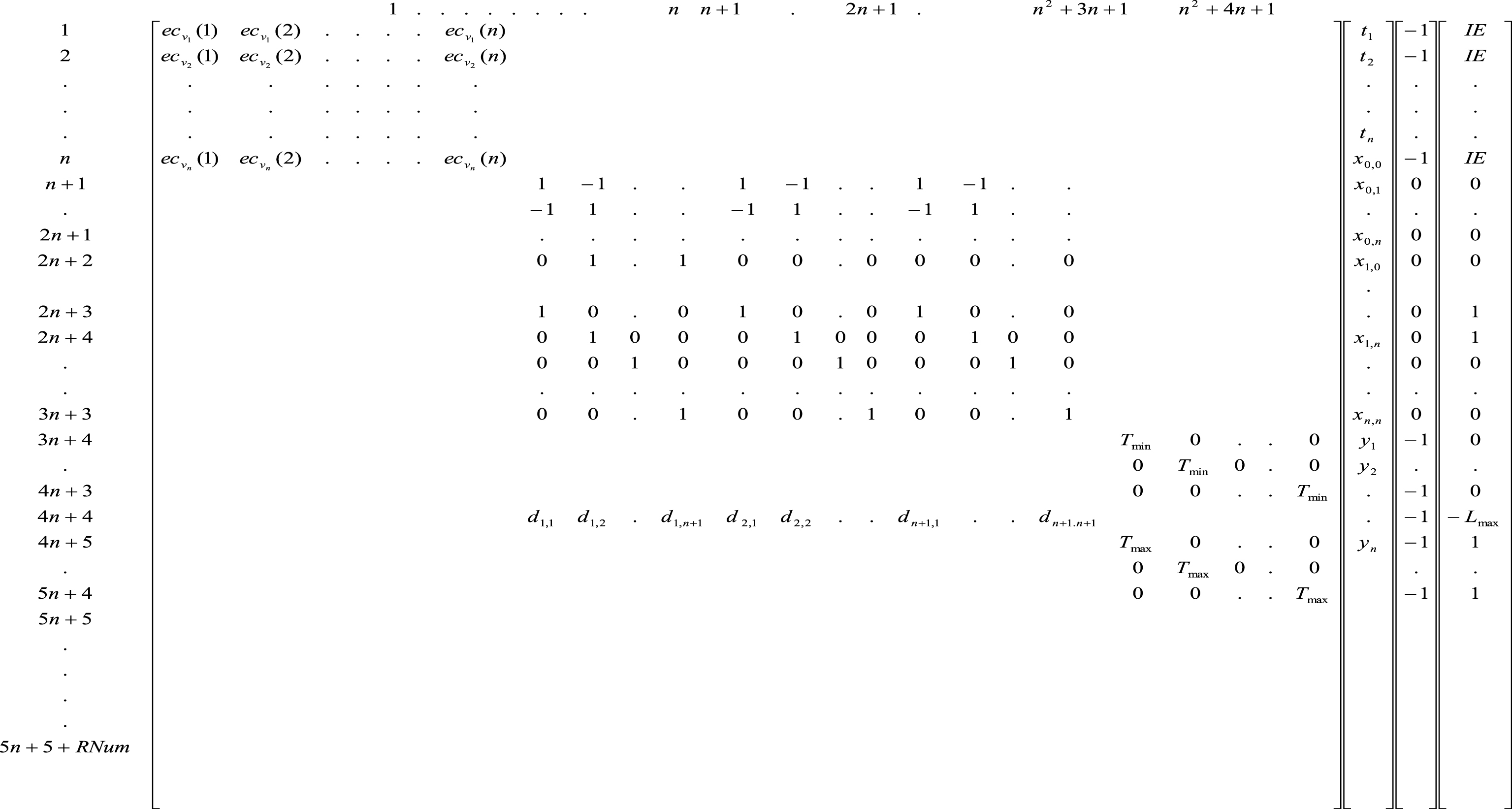
Internal structures of matrices A, f, G and B.

4.1 Mixed linear network model

The parameters and matrices of converted linear programming model are as follows:

Optimization objective: Maximize $\sum_{i = 1}^{n} t_{i}$ = Maximize $\sum_{i = 1}^{n} f_{i}$

Constraint: Distance (P_i) = ∑_{e∈P_i}D (e) ≤ L

Relationship matrix A * f G B, x ∈ [vlb, vub] is used to conduct the restriction, in which $f = z e r o s (n^{2} + 4 n + 1)^{'}$ , and its expansion is f = [t₁, t₂ …, t_n, x_0,0, x_0,1 …, x_n,0, x_n,1 …, x_n,n, y₁, y₂ …, y_n]; $\begin{matrix} A = zeros (5 n + 4 + RNum, n^{2} + 4 n + 1); \\ B = zeros (5 n + 4 + RNum, 1); \\ G = zeros (5 n + 4 + RNum, 1), \end{matrix}$ where RNum is the sum of the loops of all nodes.

Figure 1 illustrates the internal structures of matrices A, f, G and B, where the lines from 5n + 5 to 5n + 5 + RNum are the loop detection lines and the values are calculated dynamically by each node’s loop. More details are provided in Section 3.3.

4.2 Construction of relationship matrices

The constraints in Table 2 are formulated and modeled as a conditional matrix of linear programming model. The method of construction is presented as follows:

Constraint (7) is expressed as: $A (i, j) = {ec}_{v} (i, j), B (i, 1) = IE, G (i, 1) = - 1;$

Constraint (8) is expressed as: $\begin{matrix} A (n + i, n + (i - 1) \times (n + 1) + j) = 1 \\ (1 \leq i \leq n + 1, 1 \leq j \leq n + 1), \\ A (n + i, n + (j - 1) \times (n + 1) + i) \\ = - 1 (1 \leq i \leq n + 1, 1 \leq j \leq n + 1), \\ B (n + i, 1) = 0 (1 \leq i \leq n + 1), \\ G (n + i, 1) = 0 (1 \leq i \leq n + 1), \end{matrix}$

Constraint (9) is expressed as: $\begin{matrix} A (2 n + 2, n + i + 1) = 1 (1 \leq i \leq n), \\ B (2 n + 2, 1) = 1 (1 \leq i \leq n), \\ G (2 n + 2, 1) = 0 (1 \leq i \leq n); \end{matrix}$

Constraint (10) is expressed as: $\begin{matrix} A (2 n + 3, n + (i - 1) * (n + 1) + 1) = 1 \\ (1 \leq i \leq n), \\ B (2 n + 3, 1) = 1 (1 \leq i \leq n), \\ G (2 n + 3, 1) = 0 (1 \leq i \leq n), \end{matrix}$

Constraint (11) is expressed as: $\begin{matrix} A (2 * n + 3 + i, n + (j - 1) \\ * (n + 1) + i + 1) = 1 \\ (1 \leq i \leq n + 1; 1 \leq j \leq n + 1), \\ A (2 n + 3 + i, n^{2} + 3 n + 1 + i) = - 1 \\ (1 \leq i \leq n + 1) . \\ B (2 n + 3 + i, 1) = 0 (1 \leq i \leq n); \end{matrix}$

Constraint (12) is expressed as: $\begin{matrix} A (3 n + 3 + i, n^{2} + 3 n + 1 + i) \\ = T min (1 \leq i \leq n), \\ B (3 n + 3 + i, i) = - 1 (1 \leq i \leq n), \\ G (3 n + 3 + i, 1) = - 1 (1 \leq i \leq n), \\ A (4 n + 4 + i, n^{2} + 3 n + 1 + i) \\ = - 1 * T max (1 \leq i \leq n), \\ B (4 n + 4 + i, i) = 1 (1 \leq i \leq n), \\ G (4 n + 4 + i, 1) = - 1 (1 \leq i \leq n); \end{matrix}$

Constraint (13) is expressed as: $\begin{matrix} A (4 n + 4, n + (i - 1) * (n + 1) + j) = D (i, j) \\ (1 \leq i \leq n + 1; 1 \leq j \leq n + 1), \\ B (4 n + 4, 1) = L max (1 \leq i \leq n), \\ G (4 n + 4, 1) = - 1 (1 \leq i \leq n); \end{matrix}$

Constraint (14) is controlled through the upper limit value of the variables, where Lmax is the upper limit of sink movement distance; IE is the initial energy of each node; ec_v is the energy consumption coefficient of node j in the spanning tree rooted at node i, with value proportional to the number of child nodes of j node; and D (i, j) is the distance between i and j. When the sink moves to each node v_i, the node is considered as the root node to construct the data forwarding tree using the Breadth-First-Search. The number of child nodes of each node in T_i tree is also calculated to determine the energy consumption of each node when the sink sojourns at v_i.

4.3 Loop detection algorithm

In a common solving process, a potential loop may exist in a sink node’s moving path, which makes it impossible for the model to reach the global optimal solution. For this problem, the constraint strategy in [12] cannot be directly converted to relationship matrix that needs further manual verification. In order to solve this problem, a loop detection-aided algorithm is introduced in this paper. This algorithm can automatically detect and avoid the loop in a solving process by generating the constraints called by the linear programming algorithm.

Algorithm 1: Loop generation algorithm
Input: set of nodes and edges, upper limit of moving distance, number of nodes
Output: array of loop
1: Road = zeros(RoadMaxsize,n+1);
2: for each v_i ∈ V (2 ≤ i ≤ n + 1) do
3: Road(Row,1):=i;
4: TmpQuery:= zeros(RoadMaxsize,n+1); TmpQuery(1,1):=i;
5: m:= T1; k1:= i; T1:= 1; T2:= 1;
6: while m< =T1 do
7: k1:= Tail(TmpQuery(m)); % trail node of the current queue
8: for each v_j ∈ V (2 ≤ j ≤ n + 1) do
9: if k1≠j then
10: if (R(k1,j)=1) and (j not in TmpQuery(m))
{
11: if R(j,i)=1{
12: Col:= Tail(TmpQuery(m)); % trail node of current queue
13: Road(Row):= TmpQuery(m);
14: Road(Row,Col+1):= j; Road(Row,Col+2):=i;
16: Row:= Row+1;
17 }
18: T1:= T1+1; T2:= Tail(TmpQuery)+1;
19: TmpQuery(T1,T2):= j;
20: }
21: }
22: } m:=m+1;
23: }
24: }
25: }

Algorithm 1 iterates over each node. It starts from each node, accesses the adjacent nodes and generates multiple paths. It then records the path that can return to the starting point and stores them in the Road array. The Road array can be used to construct the expressions of A, B and G to avoid the loop. The ‘for’ loop from line 2 to line 25 constructs the iteration loop taking each node as the starting node. The ‘for’ loop from line 8 to line 22 realizes the selection for all potential next moving locations starting from the current node in a loop detection. The instructions from line 11 to line 16 add the nodes that meet the loop detection conditions at the end of the current row of the loop array and update the serial number of current row and column of the loop array.

The generated Road array is embodied in matrices A, B and G to avoid loops, as shown below, where Len (Road (i)) is the nonzero element number of the ith row of Road array. $\begin{matrix} A (5 n + 5 + i, n + (Road (i, j) - 1) * \\ Road (i, j + 1)) = 1 \\ (1 \leq i \leq RNum, 1 \leq j \leq n), \\ B (5 n + 5 + i, 1) = Len (Road (i)) - 1.1 \\ (1 \leq i \leq RNum), \\ G (5 n + 5 + i, 1) = - 1 (1 \leq i \leq RNum) . \end{matrix}$

4.4 Energy consumption model

First-order wireless communication model is used to calculate the consumed energy of transmitting or receiving l bits between the two nodes with distance of d. The energy consumption model is shown in Fig. 2. The energy consumptions of sending information and receiving information are calculated using Equations (16 and 17), respectively, where E_Tx-elec and E_Rx-elec are the energies consumed by sending and receiving 1 bit data, respectively. Their values are equal and can be uniformly represented by E_elec. d is the distance between the sending and receiving nodes. d_toBS is the distance between the cluster head and the base station. When d is less than d₀, automatic space path assumption model is adopted and when d is larger than d₀, multiple paths fading model is adopted. ξ_fs and ξ_amp are the energies of sending a unit data required by these two models’ power amplifiers. 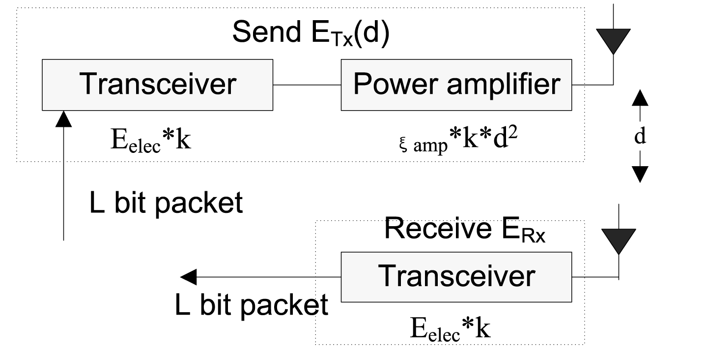$E_{Tx} (l, d) = {\begin{matrix} {lE}_{elec} + l ξ_{fs} d^{2}, d < d_{0} \\ {lE}_{elec} + l ξ_{amp} d^{4}, d \geq d_{0} \end{matrix}$ (16) $E_{Rx} (l) = E_{Rx - elec} (l) = {lE}_{elec}$ (17)

Fig.2

First-order wireless energy consumption model.

5 Model solution

In integer programming, it is called the pure integer programming or the full integer programming if all variables are restricted to be (nonnegative) integers; whereas, it is called the mixed integer programming if only one part of variables is restricted to be integer. The network in Section 3 contains connection variable sojourn time t_i of each node and integer variables x_i,j and y_i, therefore, the network is a mixed integer linear programming problem. While solving this integer programming, if the feasible region is bounded, the optimal solution can be obtained by exhausting all the feasible integer combinations of variables and then comparing their objective function values. This method is feasible and effective for small-scale problems, where the variable number and the feasible integer combination number are small. For large-scale problems, the feasible integer combination number is large, which means the exhaustive method is inadvisable. Hence, in general, a feasible method to determine the optimal integer solution is merely checking a part of the feasible integer combinations, such as branch and bound method.

Branch and bound method is a widely-used algorithm for not only discrete and combinatorial optimization problems but also for general real valued problems. The advantages of branch and bound method are: reduction of calculation while guaranteeing the precision; elimination of a large number of nodes that are unlikely to exceed the known best values, thus finally obtaining the optimal solution of problems, i.e., the best value. The basic idea of branch and bound method is to search the space of all feasible solutions (limited number) of optimization problems with constraints. During the implementation of this algorithm, all the feasible solution spaces are segmented into smaller and smaller subsets (called branch) and the next lower bound or upper bound (called delimitation) is calculated for each solution value within each subset. After each branch, the subsets whose bounds exceed the known feasible solution value will not be further segmented. Therefore, many subsets of solution (i.e., nodes on search tree) will not be considered and thus the search scope is narrowed. This process will be conducted until a feasible solution is found. This feasible solution is not larger than the bound of any subset. Generally, the optimal solution is obtained using this algorithm. Like greedy algorithm, this algorithm is also used to design the solution algorithm for combinational optimization problems. The difference is that the branch and bound method explores in the entire solution space. The time complexity of the designed algorithm is higher than that of the greedy algorithm, but its advantage is similar to the exhaustion method that can guarantee to obtain the optimal solution of the problem. In addition, this algorithm is not blind exhaustive exploration, on the contrary, it can stop further exploration for those subsets that are unlikely to obtain the optimal solution (similar to the pruning in artificial intelligence) by bounding during the exploration. Thus, it has higher efficiency than the exhaustion method. Comprehensively, considering the operations of node sorting such as father node initialization, upper bound calculation, etc., the algorithm time and space complexities both in the worst case are O (n * 2ⁿ).

Branch and bound method can be used to solve pure integer or mixed integer programming problems. Due to its flexibility and easy implementation, it has become one of the most common methods to solve integer programming. Set the integer programming problem with maximization as A and its corresponding linear programming problem as B. Starting from solving problem B, if the optimal solution does not fit the integer condition of A, the optimal objective function of B must be the upper bound of the optimal objective function Z^* of A, marked as Z^-. And the objective function value of any feasible solution of A will be a lower bound Z_- of Z^*. Branch and bound method is just a method to segment the feasible region of B into sub-regions (called branch), then gradually decrease and increase Z_-, to finally obtain Z^*.

In accordance to parameter f and relationship matrices A, B and G based on the network modeling, the branch and bound method is used to obtain the optimal programming path and the sojourn time on each node of the optimal path. The matrices A, B and G take into account of loop in the path. All the potential loops are eliminated from the matrices.

6 Simulation and analysis

6.1 Simulation environment

The WSNs simulated in this paper consists of 20 to 400 nodes that are randomly distributed in a rectangular region with length 200 m and width 150 m. The transmission range of a node is R_max = 35 m, and the initial energy IE is 50 Jules. The data collection rate of each node is set as r = 40 bits/s. In order to track additional information of energy consumption of nodes around the sink, initially the sink and the base station are both placed at (150, 100). The comparison relations of network key performance indexes are approximately similar to the situation when the sink and the base station are both located at (200, 75), middle of the right part. The energy consumption model in section 3.4 is used for the node transmission and energy. The experiment parameters are shown in Table 3.

Table 3
Main parameters of the sensor network

Parameter Description Value

N Number of nodes 15/20/25

M ₁ Network length 200 m

M ₂ Network width 150 m

E ₀ Node initial energy 50 J

E _t Energy consumed to send 1 bit data 14.4 * 10^-6

E _r Energy consumed to receive 1 bit data 5.76 * 10^-6

R _max The longest communication distance among nodes 35 m

T _min The shortest sojourn time of base station at the nodes 600 s

T _max The longest sojurn time of base station at the nodes 3000 s

L _max The longest movement distance of base station 200 m

Parameter	Description	Value
N	Number of nodes	15/20/25
M ₁	Network length	200 m
M ₂	Network width	150 m
E ₀	Node initial energy	50 J
E _t	Energy consumed to send 1 bit data	14.4 * 10^-6
E _r	Energy consumed to receive 1 bit data	5.76 * 10^-6
R _max	The longest communication distance among nodes	35 m
T _min	The shortest sojourn time of base station at the nodes	600 s
T _max	The longest sojurn time of base station at the nodes	3000 s
L _max	The longest movement distance of base station	200 m

6.2 Experimental simulation

6.2.1 Network lifetime of different scale networks with different upper limits

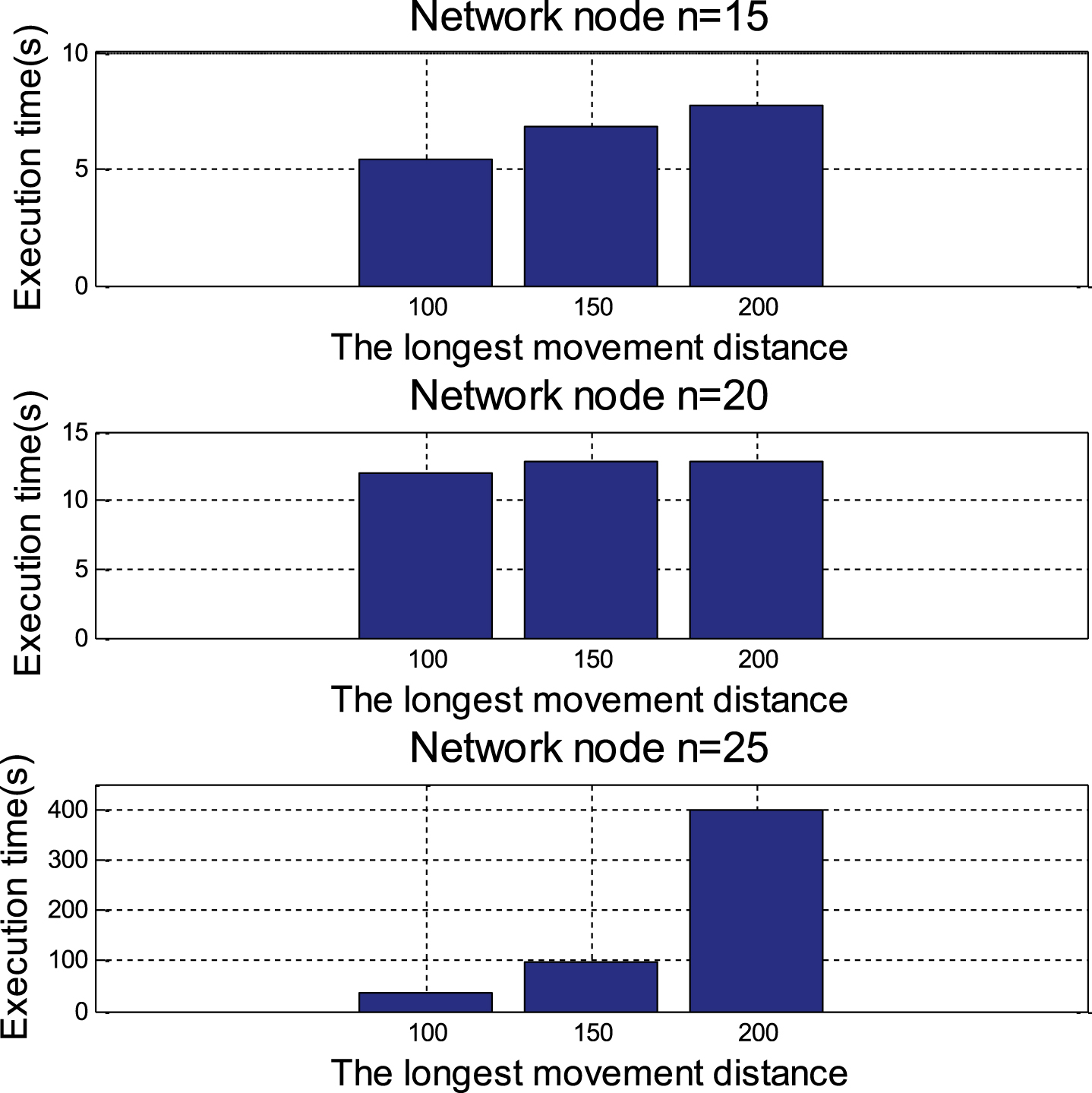
For this simulation, the network node number n is set as 15, 20 and 25, and the movement distance upper limit is set as 100, 150 and 200. The obtained simulation results of network lifetime, actual movement distance and execution time are shown in Table 4. Each value is the average value of five time continuous executions under the same network structure, which means that the randomness of data is eliminated. Table 4 shows that under different movement distance constraints, the network lifetime of the same scale network is different. The larger the movement distance upper limit is, the longer the network lifetime will be. Under the same movement distance constraints, the network lifetime decreases with increase in the network scale. The sink can sojourn more nodes with large movement distance upper limit. The nodes in different regions are regarded as neighbor nodes to balance the energy consumption of each node as data transit node. When the network is scaled up, the probability of each node as data transit node increases and the consumed energy to transmit data becomes larger than that of smaller network. Under the condition of unchanged consumed energy to transmit data, the entire energy consumption of nodes increases and the lifetime of nodes decreases slightly.

Table 4
Experimental results

Number of nodes The longest movement distance Network lifetime Movement distance Execution time

15 100 7.1152e+004s 62.3106 5.395s

15 150 7.1152e+004s 101.8589 6.781s

15 200 1.3123e+005s 183.5771 7.719s

20 100 1.0851e+005s 69.4058 12.016s

20 150 1.2860e+005s 112.6549 12.844s

20 200 1.2860e+005s 112.6549 12.844s

25 100 8.0376e+004s 96.8965 34.562s

25 150 1.0851e+005s 138.2217 97.953s

25 200 1.1098e+005s 158.7808 397.86s

Number of nodes	The longest movement distance	Network lifetime	Movement distance	Execution time
15	100	7.1152e+004s	62.3106	5.395s
15	150	7.1152e+004s	101.8589	6.781s
15	200	1.3123e+005s	183.5771	7.719s
20	100	1.0851e+005s	69.4058	12.016s
20	150	1.2860e+005s	112.6549	12.844s
20	200	1.2860e+005s	112.6549	12.844s
25	100	8.0376e+004s	96.8965	34.562s
25	150	1.0851e+005s	138.2217	97.953s
25	200	1.1098e+005s	158.7808	397.86s

Figures 3–5 present the data in Table 4 in a more intuitive way. As it can be seen from them that when the sink movement distance upper limit is increased, the network lifetime, the actual movement distance and the execution time are also increased accordingly. In particular, the algorithm execution time is rapidly increased when the network is scaled up. When the number of network nodes exceeds 50, the algorithm execution time is particularly long. For example, when n = 25 and the longest movement distance is 200, the algorithm execution time reaches 397.86, which is 30.97 times of that when n = 20. When the number of network nodes increases to a certain amount, the algorithm execution time becomes too long. This is mainly because the algorithm needs to collect data globally to obtain the optimal solution. Meanwhile, constructing network access spanning tree on each passing node will also require a certain amount of time that will be accumulated and thus will lead to a slow execution speed when the number of nodes is large.

Fig.3

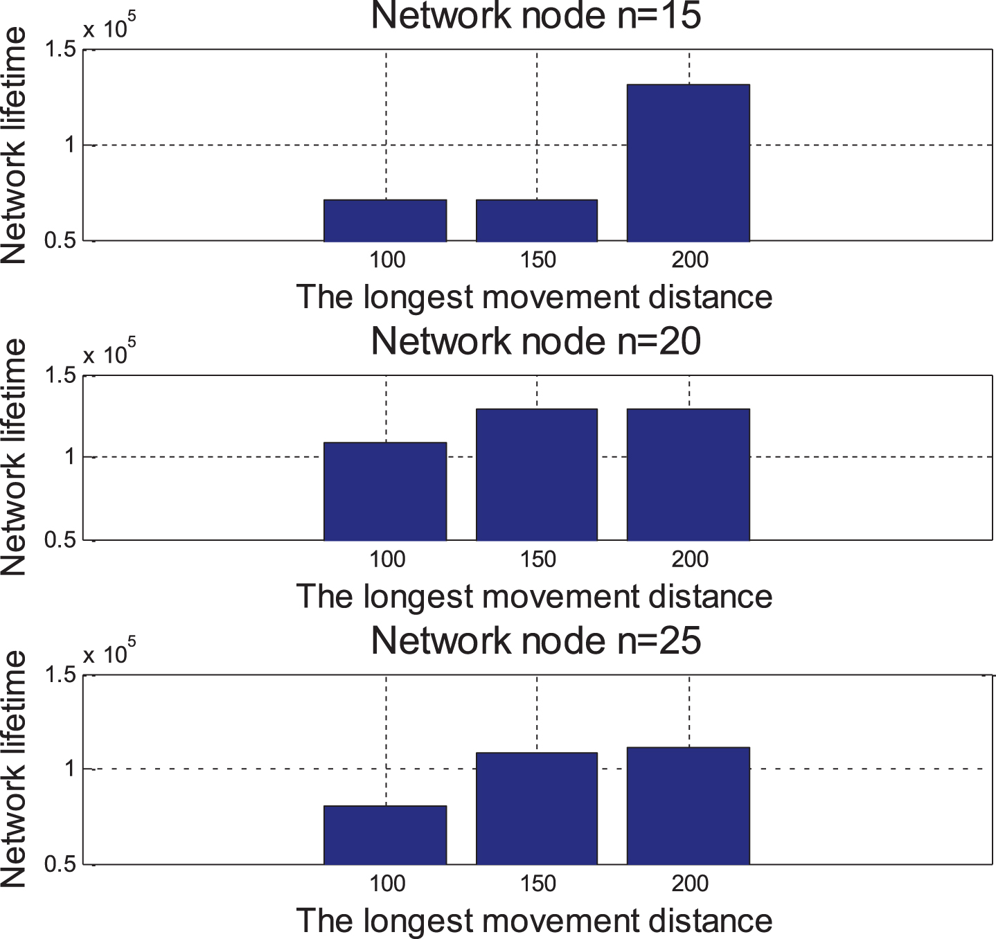
Trend of network lifetime under different longest movement distance constraints.

Fig.4

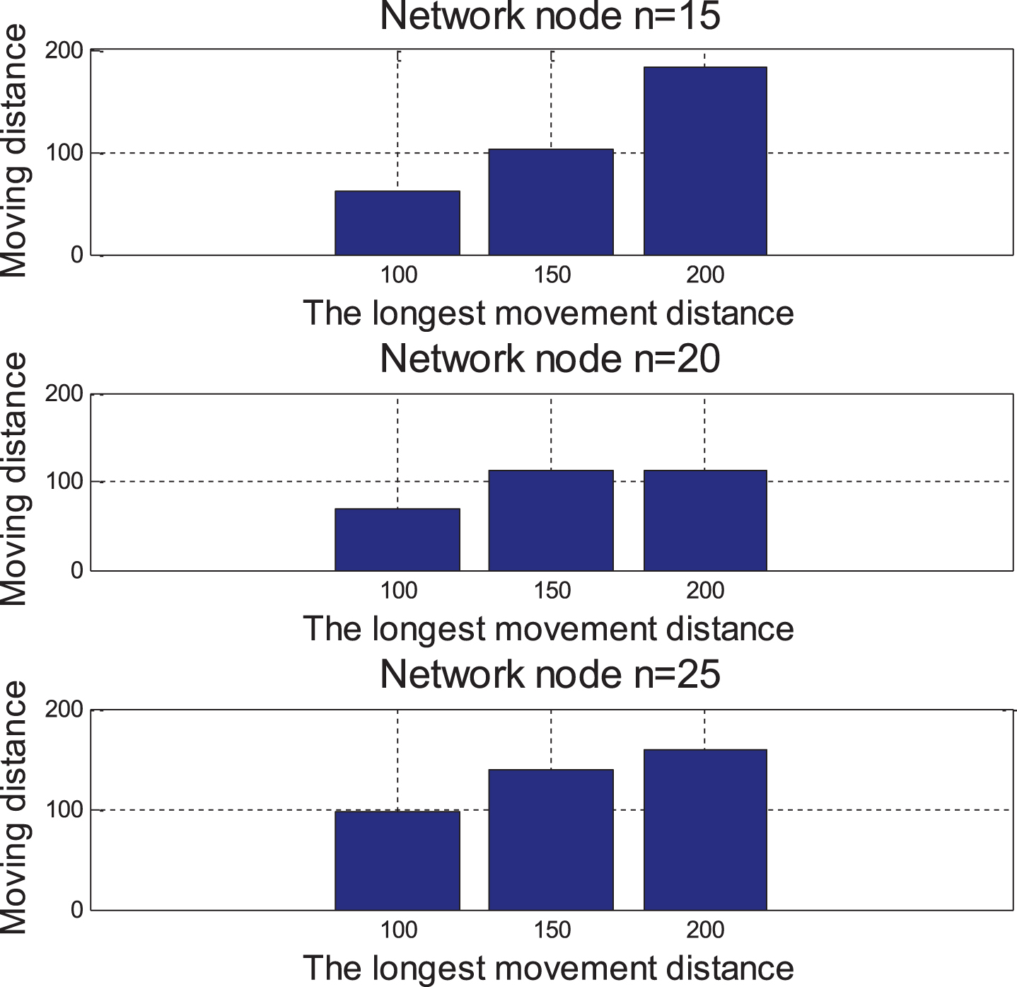
Trend of sink actual moving distance under different longest movement distance constraints.

Fig.5

Trend of algorithm execution time under different longest movement distance constraints.

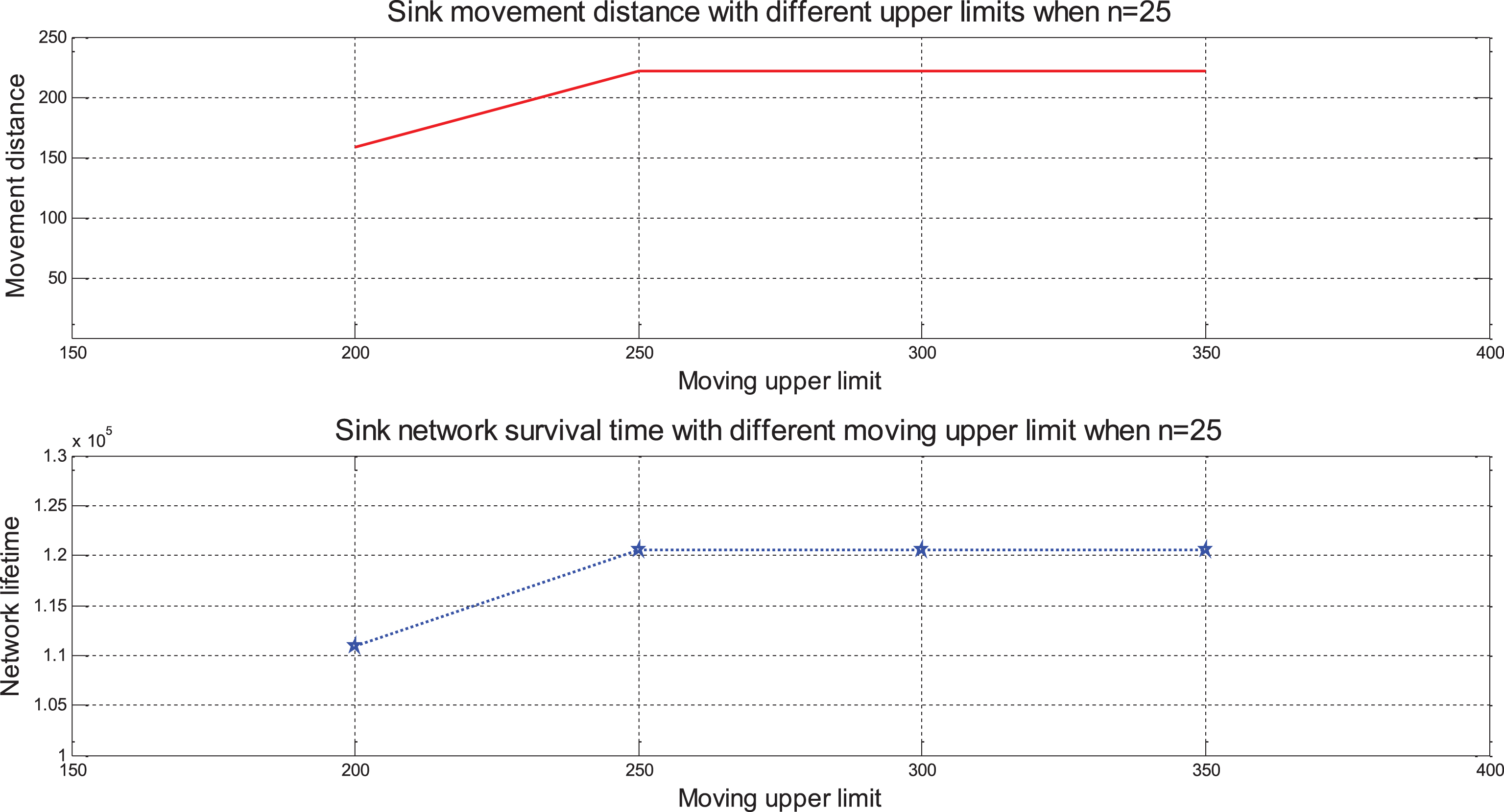
6.2.2 The influence of movement distance upper limit on network lifetime

Figure 6 and Table 5 indicate that when the sink movement distance upper limit L exceeds a certain value, it no longer affects the network lifetime. For example, when L = 250, the actual movement distance is 222.1977 and the network lifetime is 1.2055e+005. When L increases to 300 and 350, the actual sink movement distance and the network lifetime are unchanged. This is mainly because the network lifetime is restricted by multiple factors and movement distance is only one of them. Other conditions such as the initial energy of each node, the deployment density and the distribution location of nodes in network are also the key factors to restrict the network lifetime. Hence, when L is large enough, its effect on the network generated lifetime can be ignored and other constraints will determine the network lifetime.

Fig.6

Results of different sink movement distance upper limits when n = 25.

Table 5

Results of different movement distance upper limit constraints when n = 25

Moving upper limit L	Movement distance	Network lifetime	Passing modes when moving
200	158.7808	1.1098e+005	6,10,11,20,7
250	222.1977	1.2055e+005	6,10,11,20,16,2,3
300	222.1977	1.2055e+005	6,10,11,20,16,2,3
350	222.1977	1.2055e+005	6,10,11,20,16,2,3

The sink movement to new locations increases with increase in number of network nodes, and every movement requires reconstruction of access spanning tree. Thus, while solving the linear programming problems through modeling, the execution time is long and increases rapidly. The proposed model is suitable for finding the optimal path of moving sink with limited distance for small and medium scale WSNs. Further research is needed for large-scale WSNs.

7 Conclusions

In this paper, the authors have introduced a definition of communication network and have presented the network optimization objectives and constraints via conversion. The described problem has been converted into one mixed network integer linear programming by formalizing the optimization objectives into function variables of mixed programming model and converting the network constraints into constraint matrices of mixed programming model. The authors have provided detailed steps of using the branch and bound method to solve the proposed model. The analysis of experimental simulation results has shown that the network lifetime can be improved by increasing the movement distance upper limit. However, the execution time of mixed linear programming model increases rapidly when the network is scaled up. Hence, further research is required to obtain better optimized solutions.

Footnotes

Acknowledgments

This work is supported by the Natural Science Foundation (61370206), Natural Science Foundation of the Jiangsu Higher Education Institutions of China (Grant No. 16KJD510002).

References

Akyildiz

I.F.

, Su

, Sankarasubramaniam

and Cayirci

, Wireless sensor networks: A survey, Computer Networks38(4) (2002), 393–422.

Binti

M.N.N.

and Bin

A.J.

, A review of simulation framework for wireless sensor networks localization, Research and Development (SCOReD), 2014 IEEE Student Conference on, 2014.

Gaddam

, Mukhopadhyay

S.C.

and Sen

G.G.

, Wireless Sensors Networks based monitoring: Review, challenges and implementation issues, Sensing Technology, 2008 ICST 2008 3rd International Conference on, 2009, pp. 533–538.

Z.J.

, Li

, Wang

J.L.

, Cao

Z.C.

, Ubiquitous data collection for mobile users in wireless sensor networks, In: Proc of the IEEE INFOCOM Shanghai, 2011, pp. 2246–2254.

Wang

, Srinivasan

, Chua

K.C.

, Trade-Offs between mobility and density for coverage in wireless sensor networks, In: Proc Of the ACM MobiCom. Montreal, 2007, pp. 39–50.

Dantu

, Rahimi

, Shah

, Babel

, Dhariwal

, Sukhatme

G.S.

, Robomote: Enabling mobility in sensor networks, In: Proc of the IEEE IPSN Los Angeles, 2005, pp. 404–409.

Tan

C.G.

, Xu

and Wang

J.X.

, A Sink moving scheme based on local residual energy of nodes in wireless sensor networks, Journal of Central South University of Technology16(2) (2009), 265–268.

Zhang

X.W.

, Zhang

L.L.

, Optimizing energy-latency trade-off in wireless sensor networks with mobile element, In: Proc of the IEEE ICPADS Shanghai, 2010, pp. 534–541.

Ammari

, Das

, Data dissemination to mobile Sinks in wireless sensor networks: An information theoretic approach, In: Proc Of the IEEE MASS Washington, 2005, pp. 305–314.

10.

Basagni

, Carosi

, Melachrinoudis

, Petrioli

and Wang

Z.M.

, Controlled Sink mobility for prolonging wireless sensor networks lifetime, Wireless Networks14(6) (2008), 831–858.

11.

Ryo

, Rajesh

K.G.

, Optimizing energy-latency trade-off in sensor networks with controlled mobility, In: Proc of the IEEE INFOCOM Rio de Janeiro, 2009, pp. 1398–1408.

12.

Wang

, Ji

and Cheng

, Spatial-temporal Correlation-based low-latency compressed sensing in WSNs, International Journal of Grid & Distributed Computing8 (2015).