A new range-free algorithm based on hop correction of RSSI

Abstract

Referring to the issue that the hop value of the range-free DV-hop positioning algorithm could not reflect the distance between two nodes within the communication range, this paper proposes an algorithm named as HCRDV-Hop. According to the proposed algorithm, the distance measured by hops between two nodes is re-treated as the specific value with dividing the received signal strength (denoted as RSSI) between nodes with the maximum average signal strength of nodes ( ${\bar{RSSI}}_{max}$ ). Based on that, we also introduce the mathematical reasoning as well as provide the implementation procedures of the proposed algorithm. Moreover, the simulation verification is then elaborated in order to evaluate the algorithm performance. According to the simulation result, we discover that the proposed HCRDV-Hop algorithm reveals better performance in the distribution of node positioning deviations and the relative positioning deviations.

Keywords

Stereoscopic vision endoscope projection medical image

1 Introduction

Wireless sensor network is a product of computer, communication and sensor technology. It is also the product of information acquisition, information transmission and information processing. It plays an important role in many fields such as environmental monitoring, military, intelligent transportation and so on. The node positioning is a prerequisite for many applications, since the information without exact location data is meaningless to users. Therefore, the study of node location technology for wireless sensor networks is of great significance.

The performance of WSN positioning algorithms directly affects the usability. Thus it is quite necessary for a positioning algorithm to make trade-off among the multiple factors, such as the positioning accuracy, the energy consumption, etc. and also to satisfy the given requirements. Currently, a lot of positioning algorithms are proposed and they are generally categorized into the range-based and the range-free ones corresponding to the precondition whether the distance/angle between the focal nodes should be measured or not. The commonly used measurement techniques include RSSI, TOA, TDOA and AOA, etc. The range-free algorithms do not need to learn the distance and angle information between the nodes. The algorithms could position nodes relying on the connectivity between the network nodes, during which the cost for hardware could be saved. Compared with the range-based measurement algorithms, the range-free algorithms are cost-effective and thus become one of popular research issues. The range-free algorithms generally include: Centroid [4], DV-Hop) [5], APIT [6], Amorphous [7], Convex [8], etc.

In this paper, we propose the HCRDV-Hop algorithm based on the DV-hop, in which the distance measured by hops between two nodes is re-treated as the specific value with dividing the received signal strength (denoted as RSSI) between nodes with the maximum average signal strength of nodes ( ${\bar{RSSI}}_{max}$ ). In this way, we could not only reflect the distance between nodes with hops but could also decrease the deviation of the average hop distance during the treatment. At the end, we provide the verification of the algorithm.

2 Related work

2.1 DV-Hop positioning algorithm

The positioning procedures of DV-Hop algorithm consists with three phases:

(1) Calculating the minimum hops from the unknown node to every beacon node

The beacon node broadcasts a packet of its own location information to its neighbor nodes, including the hop count field, initialized to 0. Each sink node only records the minimum hops to each of the beacon nodes and ignore the other larger hop value that is received from the identical beacon node. Then it adds 1 to the received hop value and forwards the value to its own neighbors. In this way, all the nodes in network could store the minimum hop value to each beacon node.

(2) Calculating the actual distance from the unknown node to every beacon node

With the recorded location information and hop value to the other beacon node during the above mentioned phase, each beacon node estimates the actual average single hop distance according to Equation (1) and broadcasts that into the network. Each unknown node then calculates the actual distance to each beacon node according to its stored hop number after receiving the actual average single hop distance. ${HopSize}_{i} = \frac{\sum_{j \neq i} \sqrt{(x_{i} - x_{j})^{2} + (y_{i} - y_{j})^{2}}}{\sum_{j \neq i} h_{j}}$ (1)

In Equation (1), (x_i, y_i) and (x_j, y_j) are the locations of beacon nodes i, j. h_j is the number of hops between nodes i and j.

(3) Calculating the location with the likelihood estimation

The unknown node employs the maximum likelihood estimation to calculate its own location with the recorded hop distance to each beacon node obtained during the above mentioned second phase.

2.2 The existing improved DV-Hop algorithms

In citation [9], the node distance information is used as the resolution of the distance measurement and the distance between nodes is increased to improve the indirect distance measurement precision. In citation [10], the average per hop distance between beacon nodes is corrected by using the least squares criterion, and weighted average per hop distance for multi-beacon nodes used for position estimation. By setting the localization accuracy threshold, the article presents a numerical method with iterative refinement to estimate the locations of nodes. In citation [11], an algorithm named as RRDV-Hop based on the regularity of mobile anchor node (RMAN) and RSSI ranging technique is proposed. Based on the coverage ratio of two nodes, citation [12] introduced the hops coefficient, and put forward a localization algorithm based on coverage ratio. Based on the estimated distance obtained during the above mentioned third phase of DV-HOP algorithm, citation [13] provided the improvement based on the simulation curve fitting theory. In citation [14], a SRDV-Hop algorithm is proposed, in which the first hop distance to the unknown node is estimated by using RSSI.

2.3 The improved DV-Hop algorithm based on hop correction of RSSI

According to the traditional DV-Hop algorithms, one unknown node estimates the distance by hop count information between nodes and the average hop distance. Within the range of node communication, however, the number of hops is counted as one hop regardless of the actual distance, so that the nodes cannot reflect the real distance relationship between each other.

Concerning the above mentioned issue, we suggest to introduce RSSI value as one factor of revising the hop count of each node so as to improve the positioning accuracy.

Fig.1

Node distribution within the communication range.

3 Results and discussion

3.1 RSSI transmission model

The model mentioned in this paper is Shadowing model whose principle is that the signal strength will be attenuated with the distance increasing during the transmission. The model consists of two parts. The first part is path loss model that is used to predict the received signal strength (designated as P (d)) when the distance is d. The model employs the approximate distance value (designated as d₀) to the sender as the reference. Then the corresponding signal strength is P (d₀). The relation between the above mentioned variables is as following equation. $\frac{P (d_{0})}{P (d)} = {[\frac{d}{d_{0}}]}^{n}$ (2)

In real environment, the reflection, scattering, or shadowing of a signal would interferes with the signal strength at the sink node. Due to the uncertainty during signal transmission, a lot of researchers generally assume that the arrived signal strength would show a normal distribution. Under this assumption, the signal strength variation could be specified as log-normal shadowing model in further. $P (d) = P (d_{0}) - 10 η lg (\frac{d}{d_{0}}) + ξ$ (3)

In Equation (3), η represents path loss coefficient (it is usually between 2 and 4) which is of log-normal distribution. This variable is used to specify the effect onto the signal strength at the sink node. The unit of measuring P (d₀) and P (d) is designated as dBm. P (d₀) represents the RSSI value measured at the position which is 1 m far from the sending node, while P (d) represents the signal strength at the sink node.

3.2 Hop correction

In this paper, we designate the received signal strength as RSSI_max where the communication radius is R. According to Equation (3), we could induce as follows: ${RSSI}_{max} = P (d_{0}) - 10 η lg (\frac{R}{d_{0}}) + ξ$ (4)

For ease of measurement, we select to adopt Standard Normal Distribution to specify ξ: $ξ \sim N (0, σ^{2})$ (5)

Then Equation (5) is induced. $E (ξ) = 0$ (6)

The expectation of ξ is this expressed as follows:

Because the wireless signal transmission model is not of regular shape, the average signal strength at the location where the communication radius is R can be obtained with Equations (4) and (6). ${\bar{RSSI}}_{max} = E ({RSSI}_{max}) = P (d_{0}) - 10 η lg (\frac{R}{d_{0}})$ (7)

The method of correcting hop count is illustrated in Fig. 2.

Fig.2

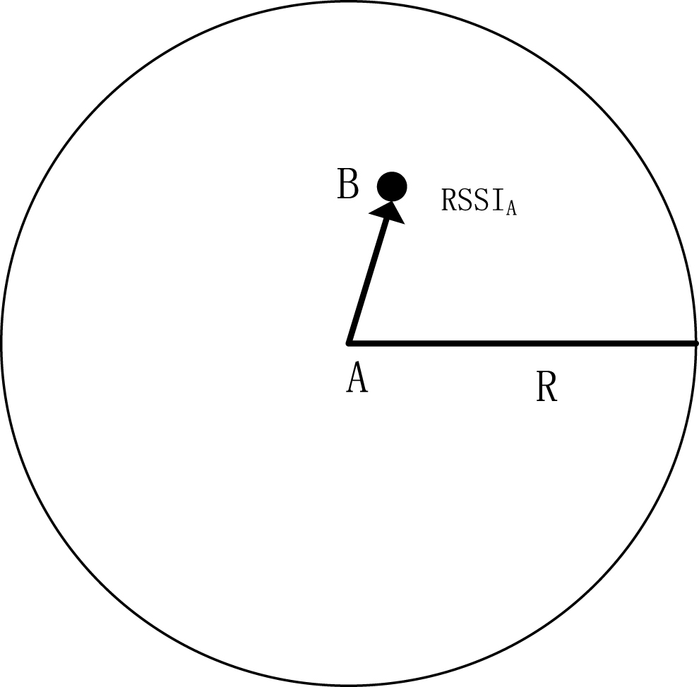
Schematic of correcting hop count.

The signal strength received at node B from node A is RSSI_A. The original DV-Hop algorithm specifies the hop count between A and B is 1, while the count is adjusted as: $H_{A} = \frac{{RSSI}_{A}}{\bar{{RSSI}_{max}}}$ (8)

From Equation (6), it can be learnt that is a decreasing function of the node communication radius R since the distance between node A and node B is less than R, i.e., AB < R, and the hop count is thus less than 1, i.e., H_A < 1. Then the hop count to any other node (denoted as i) can be expressed as: $H_{i} = \frac{{RSSI}_{i}}{\bar{{RSSI}_{max}}} \leq 1$ (9)

RSSI_max represents the maximum signal strength of node i, i.e., the signal strength at the communication radius of node i. In this way, H_i = 1 means that there exists one node at the communication radius of node i.

Let (x_i, y_i), (x_j, y_j) be the locations of the beacon nodes i and j, and let be the average hop distance of beacon nodes in the HCRDV-Hop algorithm. Then Equation (1) could be induced as follows: $\bar{{HopSize}_{i}} = \frac{\sum_{j \neq i} \sqrt{(x_{i} - x_{j})^{2} + (y_{i} - y_{j})^{2}}}{\sum_{j \neq i} H_{i}}$ (10) $\begin{matrix} = & \frac{\sum_{j \neq i} \sqrt{(x_{i} - x_{j})^{2} + (y_{i} - y_{j})^{2}}}{\sum_{j \neq i} (H_{i - 1} + \frac{{RSSI}_{i}}{\bar{{RSSI}_{max}}})} \\ = & \dots = \frac{\sum_{j \neq i} \sqrt{(x_{i} - x_{j})^{2} + (y_{i} - y_{j})^{2}}}{\sum_{i = 1}^{j \neq i} (\frac{{RSSI}_{1}}{\bar{{RSSI}_{max}}} + \dots + \frac{{RSSI}_{i}}{\bar{{RSSI}_{max}}})} \\ = & \frac{\sum_{j \neq i} \sqrt{(x_{i} - x_{j})^{2} + (y_{i} - y_{j})^{2}}}{(\bar{{RSSI}_{max}}) (\sum_{i = 1}^{j \neq i} ({RSSI}_{1} + \dots + {RSSI}_{i})} \end{matrix}$ (11)

Through analysising Equation (11), we can learn that the sum of RSSIs would become larger with the number of nodes increasing and the value of $\bar{{HopSize}_{i}}$ would turn to smaller. It implies that HCRDV-Hop algorithm would eliminate the polyline distance between nodes which could enable the estimated distance be closer, compared with the original DV-Hop algorithm, to the actual distance.

3.3 Procedures of the algorithm

to deploy the sensor nodes randomly onto the monitoring area;

Each beacon node i within the area broadcasts its own parameters including its node ID, location coordinate (x, y), the $\bar{{RSSI}_{max}}$ value at the communication radius and the initial value of H_i = 0, etc. to all the other nodes in the network;

node j within the communication radius of beacon node i receives the packet information from node i, and node j records the information from node i. Then node j updates the hop count into $H_{i} = \frac{{RSSI}_{i}}{{RSSI}_{max}}$ and forwards it to its all neighbor;

Similarly, the neighbor of the other beacon nodes scans its own data table after receiving the packets from the corresponding beacon nodes. Through comparing the multiple hop values brought by the packets from the identical beacon node, the focal node selects to store the minimum hop value and update its store corresponding hop value according to Equation (12). Then the focal node keeps forwarding the hop value to the others;

all the beacon nodes estimate the average actual distance of single hop with the other beacon nodes’ coordinates and the hop value recorded during the stet (4) according to Equation (10);

each beacon node composes its calculated average hop distance associated with the life-cycle field (i.e., TTL) in one packet and broadcasts the packet to the network in the flood mode. Each unknown node only records the particular packet whose TTL is the largest one among all the received packets from all its neighbored beacon nodes. Then the node keeps forwarding the packets to all of its other neighbors;

after having received the average distance of single hop, the node calculates the polyline distance (i.e., the multiplication of hop counts and the average distance of single hop) to each of its neighbored beacon nodes after receiving the average distance of single hop according to its stored hop count;

Unknown nodes use the polyline distance to each beacon node and calculate their coordinates using the least squares method.

4 Simulation result and analysis

4.1 Configuration of simulation

In this paper, we use MATLAB R2014a software system to analysis the performance of HCRDV-Hop algorithm. The parameters of the simulation experiment are stated in the following table.

Table 1
Parameters of the simulation experiment

Plan 1 Plan 2

The target area (m²) 100100 100100

Sum of nodes 200 200

Communication model LAM LAM

Communication radius 35 20,25,30,35,40

Number of beacon nodes 40,50,60,70,80 60

Reference algorithms for comparison DV-Hop, Amorphous, HCRDV-Hop DV-Hop, Amorphous, HCRDV-Hop

	Plan 1	Plan 2
The target area (m²)	100*100	100*100
Sum of nodes	200	200
Communication model	LAM	LAM
Communication radius	35	20,25,30,35,40
Number of beacon nodes	40,50,60,70,80	60
Reference algorithms for comparison	DV-Hop, Amorphous, HCRDV-Hop	DV-Hop, Amorphous, HCRDV-Hop

The total number of nodes in the simulation experiment is 200; the distribution area is 100×100 (unit: m²); the communication model between nodes is LAM. In this paper, HCRDV-Hop algorithm is compared and evaluated with DV-Hop algorithm and Amorphous algorithm.

The proposed algorithm does not need to measure, and it could only execute positioning relying on the connectivity. During the usage, the requirements onto hardware are simple, and the algorithm is easy to implement. In the paper, we evaluate the performance of the proposed algorithm through investigating its relative positioning deviation and the distribution of the positioning deviations.

The positioning deviation of node n is expressed as: ${Err}_{n} = \sqrt{(x_{n}^{⌢} - x_{n})^{2} + (y_{n}^{⌢} - y_{n})^{2}}$ (12)

In Equation (12), $(x_{n}^{⌢}, y_{n}^{⌢})$ is the actual coordinate of node n, while (x_n, y_n) is the estimated coordinate by the algorithm.

The relative deviation can be induced by: $Δ \bar{Err} = \frac{\sum_{i = 1}^{N} {Err}_{i}}{NR}$ (13)

In Equation (13), N represents the sum of the unknown nodes, while R represents the communication radius.

The experiment is divided into two plans, and each plan is divided into five rounds, and each round is executed for 100 times.

Plan 1: the communication radius is configured as R = 35 m, and the numbers of the beacon nodes along the multiple rounds are 40, 50, 60, 70 and 80. During executing the plan, we will analyse the relation between the beacon node count and the relative positioning deviation as well as the influence released from the beacon node count onto the distribution of the positioning deviations.

Plan 2: the number of beacon nodes is fixed as 60, and the communication radius is set 20 m, 25 m, 30 m, 35 m and 40 m during the multiple rounds. We will also analyse the issues mentioned in plan 1.

4.2 Plan 1

Figure 3 presents the influence released from the beacon node count onto the distribution of the positioning deviations. Although the number of beacon nodes increases, the relative positioning deviations of the three investigated algorithms decrease a little and turn to stable. Through comparing the proposed HCRDV-Hop algorithm with the original DV-Hop algorithm, they both decease slowly and then turn to stable, during which the deviation of the former is always less than the latter by 9.2% to 10%. Referring to the comparison between HCRDV-Hop and Amorphous, the deviation of the latter increases a little at beginning and then turn to smaller since the number of beacon nodes is 60, while the deviation of the former keeps decreasing and it is always less than the latter by 5% to 8%.

Fig.3

Comparison of positioning accuracy in plan 1.

Fig.4

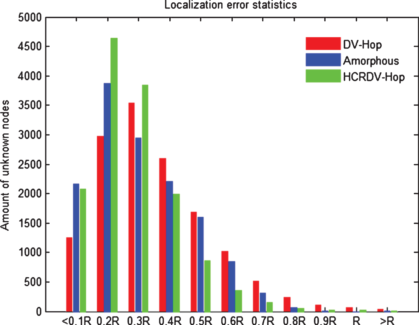
Error distribution with 40 anchors & R = 35 m.

Fig.5

Error distribution with 50 anchors & R = 35 m.

Fig.6

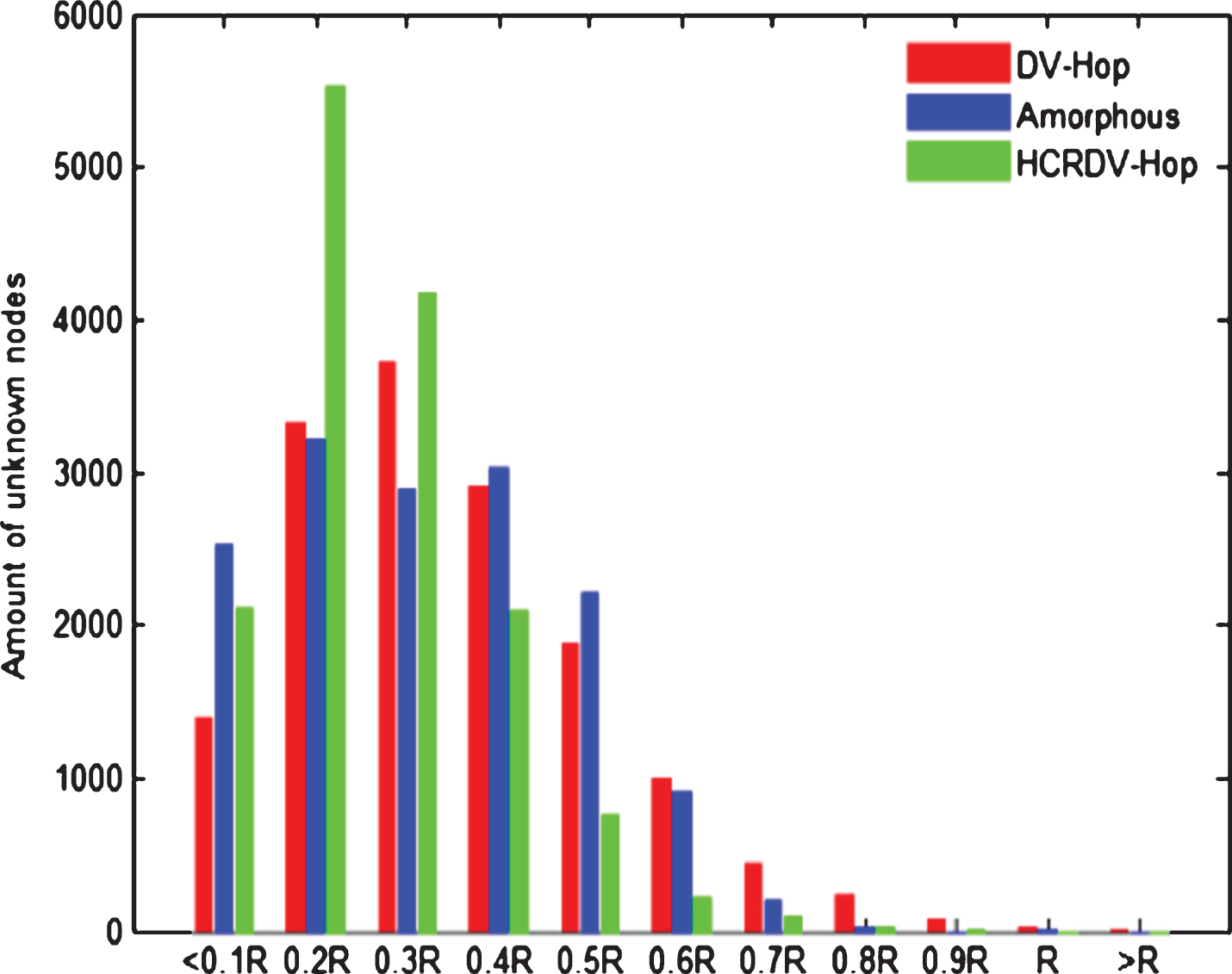
Error distribution with 60 anchors & R = 35 m.

From the figures illustrating the distribution of deviations, the average deviations of unknown nodes brought in by HCRDV-Hop algorithm mainly spread within 0.1 R to 0.4 R of the low area along the number of beacon nodes varies from 40 to 70. Meanwhile, the average deviations brought in by Amorphous algorithm always spread within 0.1 R to 0.5 R, while the average deviations brought in by DV-Hop algorithm is spread within 0.1 R to 0.6 R. Therefore, the deviations brought in by HCRDV-Hop algorithm are relatively small and vary weakly.

4.3 Plan 2

As illustrated in Fig. 7, the positioning deviation of HCRDV-Hop algorithm decreases with the communication radius increasing, during which the positioning deviation brought in by HCRDV-Hop algorithm is always less than DV-Hop algorithm by 7% to 11%. Along the communication radius increases from 20 m to 40 m, the deviation brought in by HCRDV-Hop algorithm declines sharply from 27% to 17%. Compared with DV-Hop, Amorphous algorithms, with the radius increasing, HCRDV-Hop algorithm is in better performance. Especially when the radius is 40 m, the deviation brought in by HCRDV-Hop algorithm is less than the other two algorithms by about 10%.

Fig.7

Error distribution with 70 anchors & R = 35 m.

Fig.8

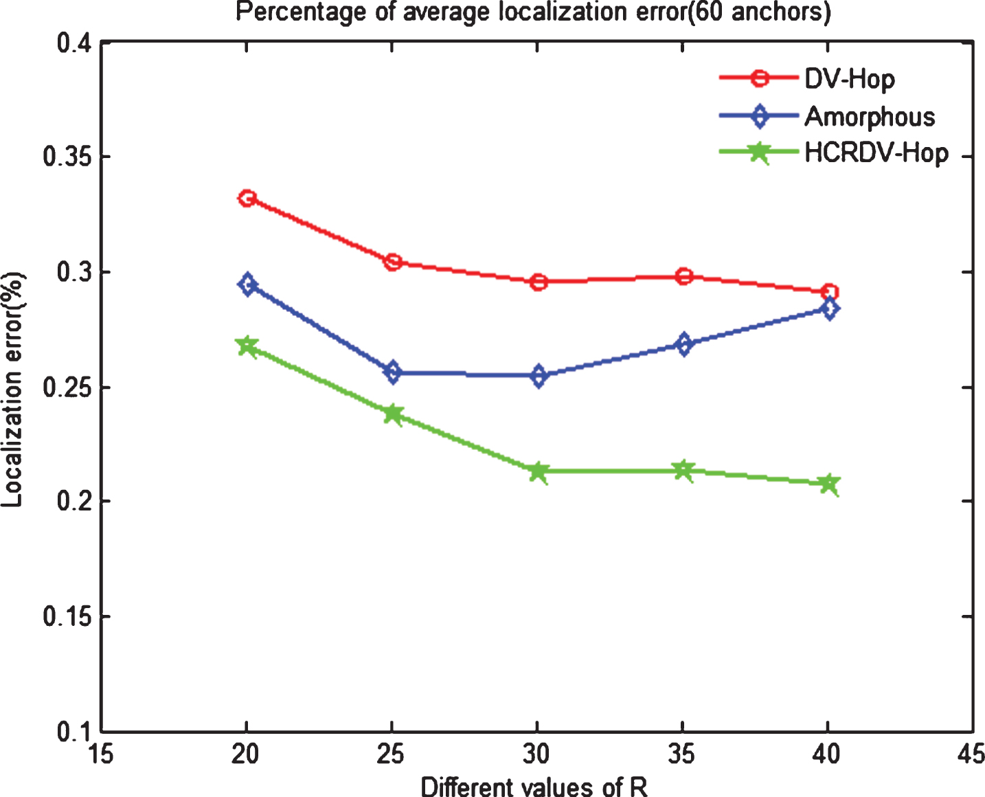
Localization accuracy comparison of plan 2.

Fig.9

Error distribution with 60 anchors & R = 25 m.

Fig.10

Error distribution with 60 anchors & R = 30 m.

Fig.11

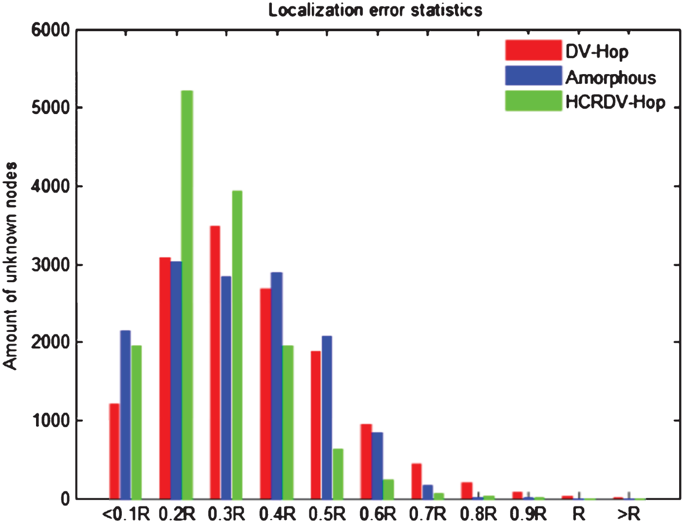
Error distribution with 60 anchors & R = 35 m.

Fig.12

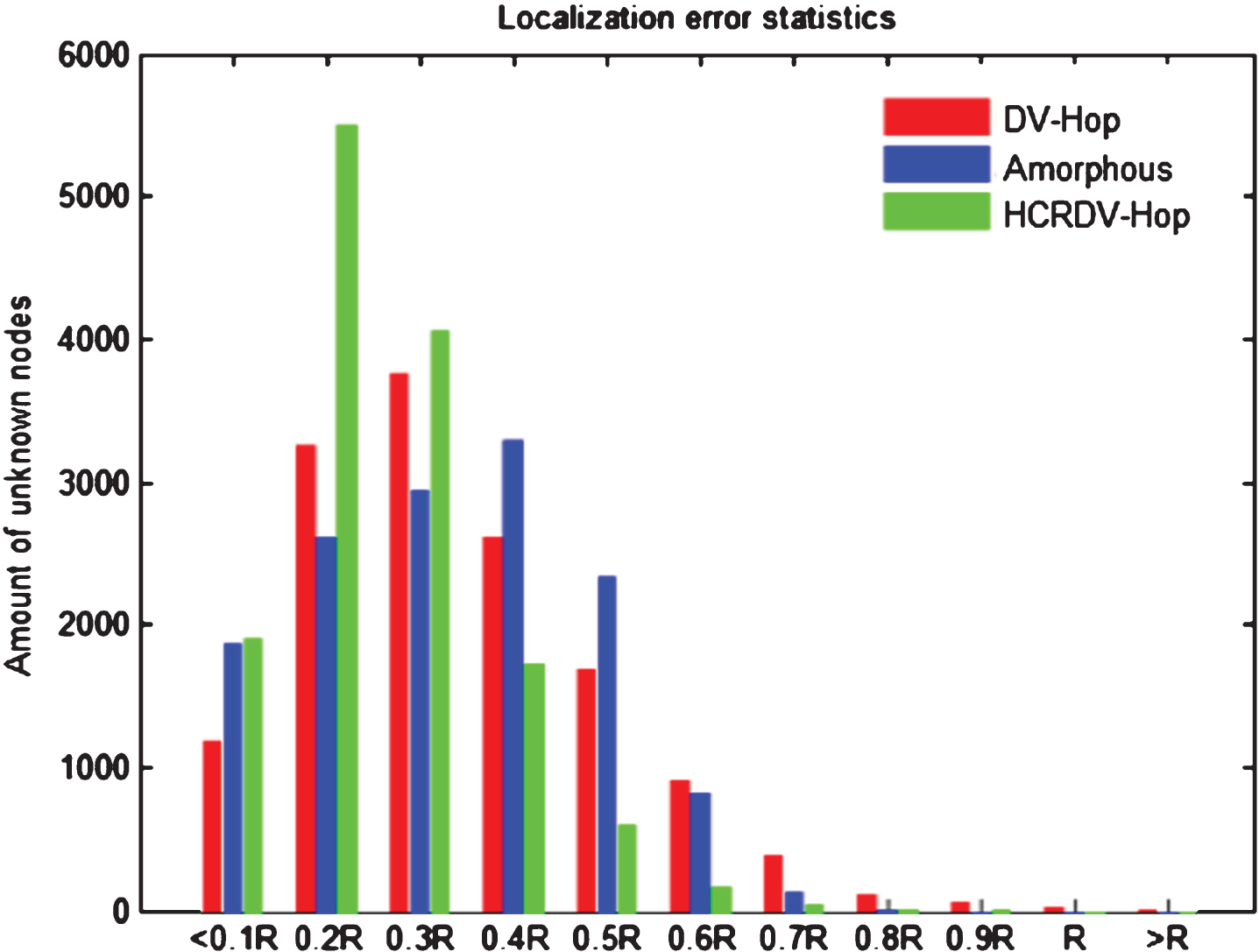
Error distribution with 60 anchors & R = 40 m.

From the figures illustrating the distribution of deviations, the average deviations of unknown nodes brought in by HCRDV-Hop algorithm mainly spread within 0.1 R to 0.4 R of the low area along the communication radius varies from 24 m to 40 m. Meanwhile, the average deviations brought in by Amorphous algorithm always spread within 0.1 R to 0.6 R, while the average deviations brought in by DV-Hop algorithm is spread within 0.1 R to 0.7 R. Therefore, the deviations brought in by HCRDV-Hop algorithm are relatively small and vary weakly.

5 Conclusion

To improve the positioning performance of DV-Hop algorithm within the random -distributed-sensor network, the hop count in the algorithm is adjusted and the distance measured by hops between two nodes is re-treated as the specific value with dividing the received signal strength (denoted as RSSI) between nodes with the maximum average signal strength of nodes ( ${\bar{RSSI}}_{max}$ ). As specified by the simulation experiment, either the communication radius or the ratio of anchor nodes varies, the improved algorithm could bring in less positioning deviation than the original one by 7% to 10%. Moreover, the deviation values brought in by most of the unknown nodes are distributed within 0.1 R to 0.4 R, and the number of unknown nodes that exist within 0.1 R to 0.2 R is more than half.

References

Akyildiz

I.F.

, Su

and Sankarasubramaniam

, Wireless sensor networks: A survey, Computer Networks the International Journal of Computer & Telecommunications Networking38(4) (2002), 393–422.

Wang

F.B.

, Shi

and Ren

F.Y.

, Self-localization systems and algorithms for wireless sensor networks, Journal of Software16(5) (2005), 857.

Duan

W.J.

, Wang

J.G.

and Wang

F.B.

, Research and development of localization systems and algorithms for wireless sensor networks, Information & Control35(2) (2006), 239–245.

Bulusu

, Heidemann

and Estrin

, GPS-less low cost outdoor optimization for very small devices, IEEE Personal Communications7(5) (2000), 28–34.

Niculescu

and Nath

, DV based positioning in ad hoc networks, Telecommunication Systems22(1) (2003), 267–280.

, Huang

, Blum

B.M.

, et al., Range-free localization schemes for large scale sensor networks, International Conference on Mobile Computing and Networking, MOBICOM 2003, San Diego, Ca, USA, DBLP, 2003, pp. 81–95.

Nagpal

, Shrobe

and Bachrach

, Organizing a Global Coordinate System from Local Information on an Ad Hoc Sensor Network, Information Processing in Sensor Networks, Second International Workshop, IPSN 2003, Palo Alto, CA, USA, Proceedings 2003, 2003, pp. 333–348.

Doherty

, Pister

K.S.J.

and Ghaoui

L.E.

, Convex position estimation in wireless sensor networks, INFOCOM 2001 Twentieth Joint Conference of the IEEE Computer and Communications Societies Proceedings IEEE IEEE, vol. 3, 2002, pp. 1655–1663.

Zheng

M.C.

, Zhang

D.F.

and Zhao

J.Q.

, Distance estimating algorithm based on gradient neighbors in wireless sensor networks, Journal on Communications29(11) (2008), 237–245.

10.

Lin

J.Z.

, Chen

X.B.

and Liu

H.B.

, Iterative algorithm for locating nodes in WSN based on modifying average hopping distances, Journal on Communications30(10) (2009), 107–113.

11.

Rui-Xue

L.I.

, Fang

Z.Y.

and Ting-Ting

Y.I.

, Improved DV-Hop localization algorithm based on regularly moving anchor(RMAN) and received signal strength indicator(RSSI) and its performance analysis, Journal of Jilin University41(2) (2011), 435–441.

12.

Tan

and Zhang

, Improved DV-hop localization algorithm based on coverage of nodes, Journal of Beijing University of Posts & Telecommunications37(1) (2014), 35–38.

13.

Liu

, Feng

, Zhang

, et al., A new range-free localization algorithm based on amendatory simulation curve fitting in WSN, International Journal of Distributed Sensor Networks2015 (2015), 1–9.

14.

Wongkhan

and Chantaraskul

, Selected RSSI-based DV-Hop localization for wireless sensor networks, 2015.

15.

Boudhir

A.A.

, Bouhorma

and Mohamed

B.A.

, New technique of wireless sensor networks localization based on energy consumption, International Journal of Computer Applications9(12) (2010), 24–28.

16.

, Liu

, Lang

, et al., Distance measurement model based on RSSI in WSN, Wireless Sensor Network2(8) (2010), 606–611.

17.

Kumar

, Reddy

and Varma

, Distance measurement and error estimation scheme for RSSI based localization in Wireless Sensor Networks, Wireless Communication and Sensor Networks IEEE, 2010, pp. 1–4.

18.

Fang

, Zhao

, Geng

, et al., RSSI variability characterization and calibration method in wireless sensor network, IEEE International Conference on Information and Automation IEEE, 2010, pp. 1532–1537.

19.

Zheng

, Wu

, Chu

, et al., Localization Algorithm Based on RSSI and Distance Geometry Constrain for Wireless Sensor Network, International Conference on Electrical and Control Engineering IEEE Computer Society, 2010, pp. 2836–2839.

20.

Feng

, Gao

, Yang

, et al., Fuzzy distance measuring based on RSSI in Wireless Sensor Network, International Conference on Intelligent System and Knowledge Engineering IEEE, 2008, pp. 395–400.