Mouth and eyebrow segmentation for emotion recognition using interpolated polynomials

Abstract

Facial Expression Recognition (FER) is a research area that has been interesting for computer science community in recent years. In this paper, we propose a methodology for the three stages of a FER system. In the pre-processing stage a method based on edge detectors and thresholding operators for eyebrow and mouth segmentation is proposed; the next stage is feature extraction, we propose using polynomials as features for describing eyebrows and mouth regions. Finally, in classification stage different supervised learners such as: Neural Networks, K-Nearest Neighbors and C4.5 decision trees are tested in order to obtain a model for classifying three out of six basic emotions (anger, happiness and surprise). According to our results, the proposed approach has acceptable accuracy for predicting new examples.

Keywords

Expression recognition face images pre-processing supervised classification interpolation features

1 Introduction

Nowadays, artificial intelligence has been an interesting area of computer science, then in combination with the analysis/processing of images computer vision was emerged. An application of computer vision is emotion recognition, that extracts information from images to recognize the emotion of a person such as: happiness, anger or surprise.

Image processing is based on applying different filters to extract relevant information from an image or a set of images (video), commonly the used filters are related to: border extraction, smoothing filters, threshold operators, gray scale conversion, among others. When a filter is applied over a image, every pixel is processed (point filter), then the region based filters take into account the neighbors of the pixel to modify its intensity. These processes could be computationally expensive, for that reason parallel approaches could be a good alternative.

An application in computer vision area is Facial Expression Recognition (FER), this application is based on extracting information from a face image using digital image filters, then characteristic attributes from the Regions Of Interest (ROIs) such as: eyes, eyebrows and mouth are extracted in order to build a model within a supervised learner to classify new instances.

Commonly, FER system consist of three stages: pre-processing, feature extraction and classification. In the first stage of a FER system the images need to be processed for detecting border information of the ROIs (in this case eyebrows and mouth), filters such as edge detectors, automatic contrast adjustment, color model transformation, among others are applied. In this stage some of the ROIs are segmented in order to obtain a binary image with the region.

The feature extraction stage obtains descriptive information about the segmented regions. In general, points of the ROIs are used to find distances or angles between some of them. In this paper interpolated polynomials are used for extracting features such as coefficients or points which are used as input training for supervised learners to find a model that have acceptable accuracy to classify three of the six basic emotions (happiness, surprise and anger).

For classification purposes a supervised learner is used to generate a model for classify or predict new examples, In this work, we use the following learning methods: Decision trees, K-Nearest Neighbor (K-NN) and feed forward Neural Networks (NN).

Commonly, FER systems are designed to analyze the six universal emotions that were presented by Paul Ekman in 1994 [1], these emotions are: happiness, anger, sadness, disgust, surprise and fear. Besides these expressions some authors consider the neutral state. Other contribution of Ekman is the FAcial expression Coding System (FACS), this system provides a description of movements in the face given a time window to detect it; those are called Actions Units (AU). FACS specifies 9 AUs in the upper region and 18 for the lower one; in addition, there are 14 head positions, 9 eye positions, 5 miscellaneous AUs, 9 action descriptors, 9 gross behavior and 5 visible codes [2].

In this work we propose an approach for segmenting eyebrows and mouth regions based on edge detectors and thresholding operators; then, features for describing the segmented ROIs are extracting by interpolation process to train supervised learners. In order to determine the classifier that has the best performance, different experiments and comparisons are reported.

This paper is structured in five sections: Section 2 describes some related works about FER; in Section 3 the proposed methodology is presented; Section 4 shows the results of each stage. Finally, conclusions and future work are described in Section 5.

2 Related works

In recent years, deep learning approaches are followed by researchers in order to get higher accuracy in their works. An approach of this kind applies in pre-processing stage a resizing filter to get 48 × 48 pixels and different learners are used to extract features from face images, then other classifiers are applied for testing these features [3]. Convolutional Neural Networks (CNN) are used with selected areas of the face as input, they have good performance to classify examples [4]. Deep Belief Networks (DBN) are used for splitting face images in different parts, then different architectures are experimented having a good performance compared with ensembles based on SVM and Adaboost classifiers [5].

A method based on edge detectors shows a comparison among four edge detectors (Robert, Sobel, Laplace and Canny), the authors report that the best performance is obtained by Canny edge detectors [6]. Other work based on a pyramid approach getting a set of resized images as feature uses decision trees in classification stage [7]. Local Binary Patterns (LBP) histogram also have been used as features of an SVM learner, then the six basic emotions are classified [8]. Siddiqi et al. [9] use Hidden Markov Models to classify, in the pre-processing stage a equalization of the histogram is used to improve the image quality, then a wavelet transform is applied over face images and the result is used as feature. In the experimental results high precision in classification process is reported.

A parallel implementation is reported by George Sabu [10], he uses Graphic Processing Units (GPU) in pre-processing stage. Important points of ROIs are found in the processed image, then distances and angles are used as features, for classification process SVM learner is used. Rahulamathavan et al. [11] present an approach where principal component analysis and local fisher discriminant analysis are used to encrypt a face image, then the output of these encrypted function is the input for a distance-based classifier.

Emotion recognition is not limited to digital image processing, audio processing could be used to classify the emotion that a person is showing, an example of audio it is presented by Pell et al. [12], they take into account both audio wave with different filters, and speech to recognize the emotion of a person.

3 Proposed methodology

The proposed methodology for segmenting and extracting features from face images consists of three stages that can be seen in Fig. 1: first, either RGB or gray scale images can be used as input of the FER system; then, in the pre-processing stage different improvements of thresholding techniques and edge detectors are applied in order to obtain descriptive information of ROIs; in the feature extraction stage interpolation algorithms are used to get coefficients and points used as input of learners; finally, different learners are tested to evaluate the features extracted from the second stage. In the following sections each stage of our approach is described.

Fig.1

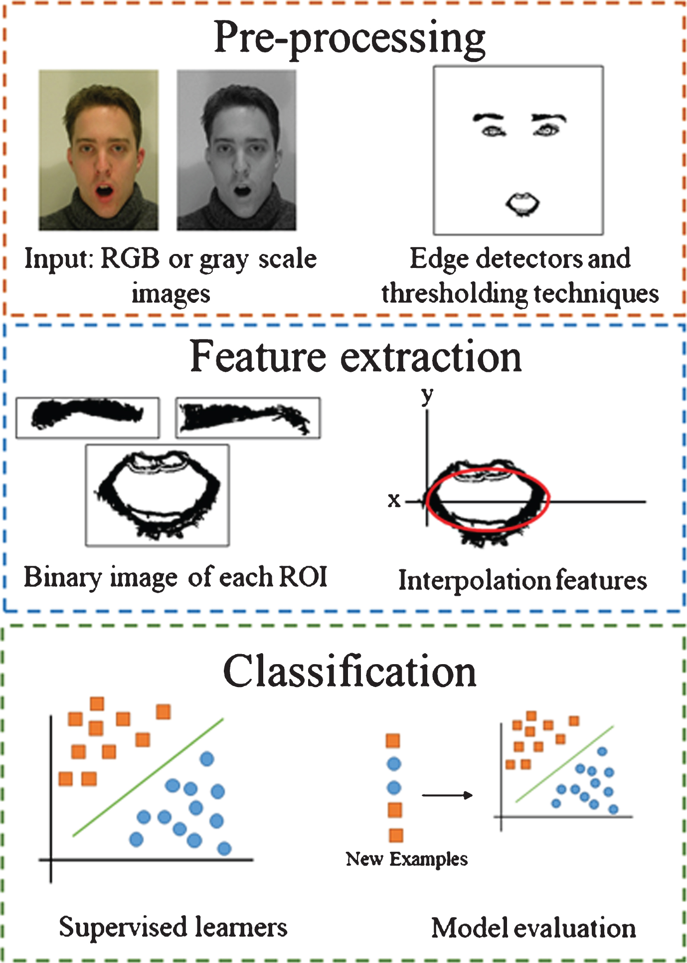
General flow diagram of the proposed methodology.

3.1 Pre-processing

In the pre-processing stage, a process based on edge detectors and thresholding techniques are proposed in order to segment mouth and eyebrows regions; different process for each region is applied.

In order to reduce the number of pixels that will be processed, the Viola & Jones algorithm [14] is used to find the face region in a digital image, this algorithm uses the intensity values of eyes and mouth regions (these regions are darker than others in face images). After the face region is located in the image, a mask using geometric information of the face is applied to approximate the region where the ROIs are located. An example of the used mask can be seen in the Fig. 2. This mask is used to define the regions that will be analyzed to reduce the number of pixels to process.

Fig.2

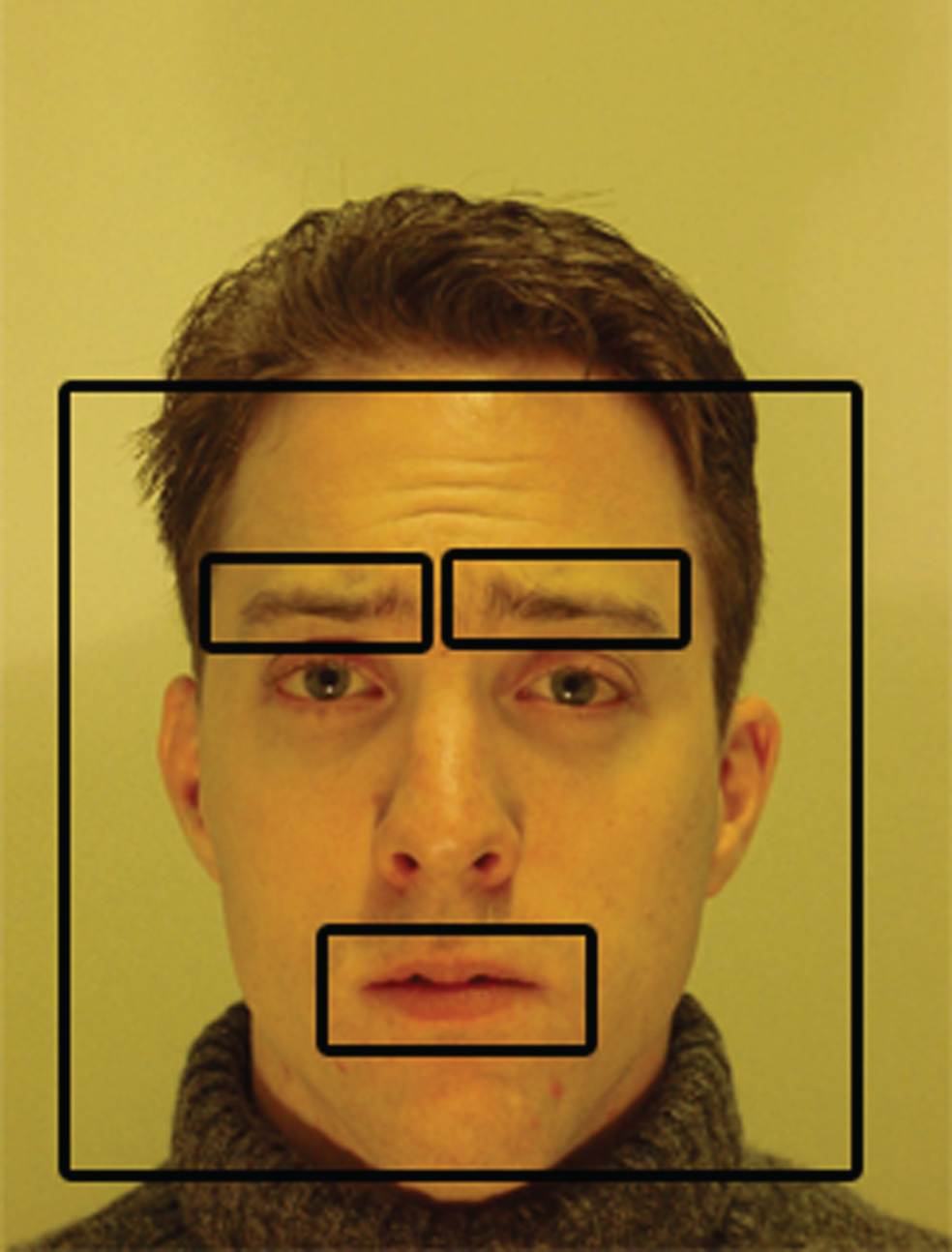
Example of the mask used to find the ROIs, images were taken from MMI dataset [13].

We note that each channel of the RGB color model provides different information about borders of ROIs, red and green channel are used to segment mouth and eyebrows regions. For eyebrow region red channel intensity values in a gray scale image are processed, the process can be seen in Algorithm 1 (ERED, Eyebrow REgion Detection). In this case a shadow between eye and eyebrow region needs to be removed in order to separate the regions. To deal with this problem an hyperbolic tangent operator is used to improve the contrast in the image (line 2), then the threshold operator of Equation 1 (where f′ (x, y) is the sine filter and f (x, y) is the same value of the pixel) is used to separate eyebrow and eye region (lines 2–5). After that, a closing morphological filter for gray scale images is applied to eliminate thin holes and as a smoothing filter with the structure element that is shown in Fig. 3 (line 6). Finally, Otsu thresholding algorithm [15] are used to binarize the image (lines 7–14), Otsu algorithm finds separability of two regions in the histogram having as output a threshold value, then this value is used to binarize the image. $f (x, y) = {\begin{matrix} f (x, y) & if & f (x, y) \leq threshold \\ f^{'} (x, y) & if & f (x, y) > threshold \end{matrix}$ (1)

Fig.3

Structure element commonly used in morphological operators.

Algorithm 1

Eyebrow REgion Detection (ERED) algorithm.

Require: Image in RGB color model I
Ensure: Binary image with eyebrow region I_s
1: Separate the channel of I {I_R, I_G, I_B}
2: Apply hyperbolic tangent filter to I_R.
3: for each value in I_Rdo
4: Apply threshold filter of Equation 1
5: end for
6: Apply closing morphological filter with the structure element of equation 3 I_M
7: Compute the Histogram H of I_M and apply Otsu algorithm to get a threshold th
8: for each value x in I_Rdo
9: ifx is minor than ththen
10: the new pixel value will be 255
11: else
12: the new pixel value will be 0
13: end if	14: end for	15: Return new image I_s

For mouth segmentation EDEM (Edge DEtection in Mouth) algorithm is proposed (see Algorithm 2), here two gray scale images are processed with the same filters (in this case red and blue channels intensity values). For this process, region based filters are improved taking into account a higher region, the region for convolution process has dimension (2u + 1) x (2u + 1), where u is the value that defines the size of the convolutional mask; we use the gradient edge detector in two directions (horizontal and vertical) with the convolutional masks of Fig. 4, then the magnitude between these two values is found, in order to enhance the border transitions in the image a sine filter is applied (lines 2–7). The histogram is used to remove the noise, considering as noise frequency those values lower than the mean respect to intensity values (lines 10–14). Up to this point, two regions in the histogram are defined and a binarization process with value = 127 is applied (line 15).

Fig.4

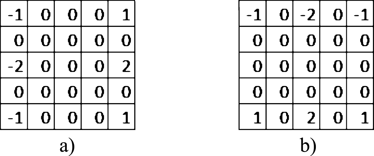
Convolutional Masks for edge detection with u = 2: a) horizontal; b) vertical.

The output of the Algorithms ERED and EDEM is a binary image containing the ROI and some noise (eye region and hair for the case of eyebrows, nose for mouth and beard in some instances). To deal with this problem an algorithm based on dbscan clustering [16] is proposed, for this case we consider as dense region (cluster). Those black regions in a binary image as can be seen in Fig. 5, in Fig. 5b the clusters in the image are depicted in a different color, Fig. 5a shows the original binary image.

Fig.5

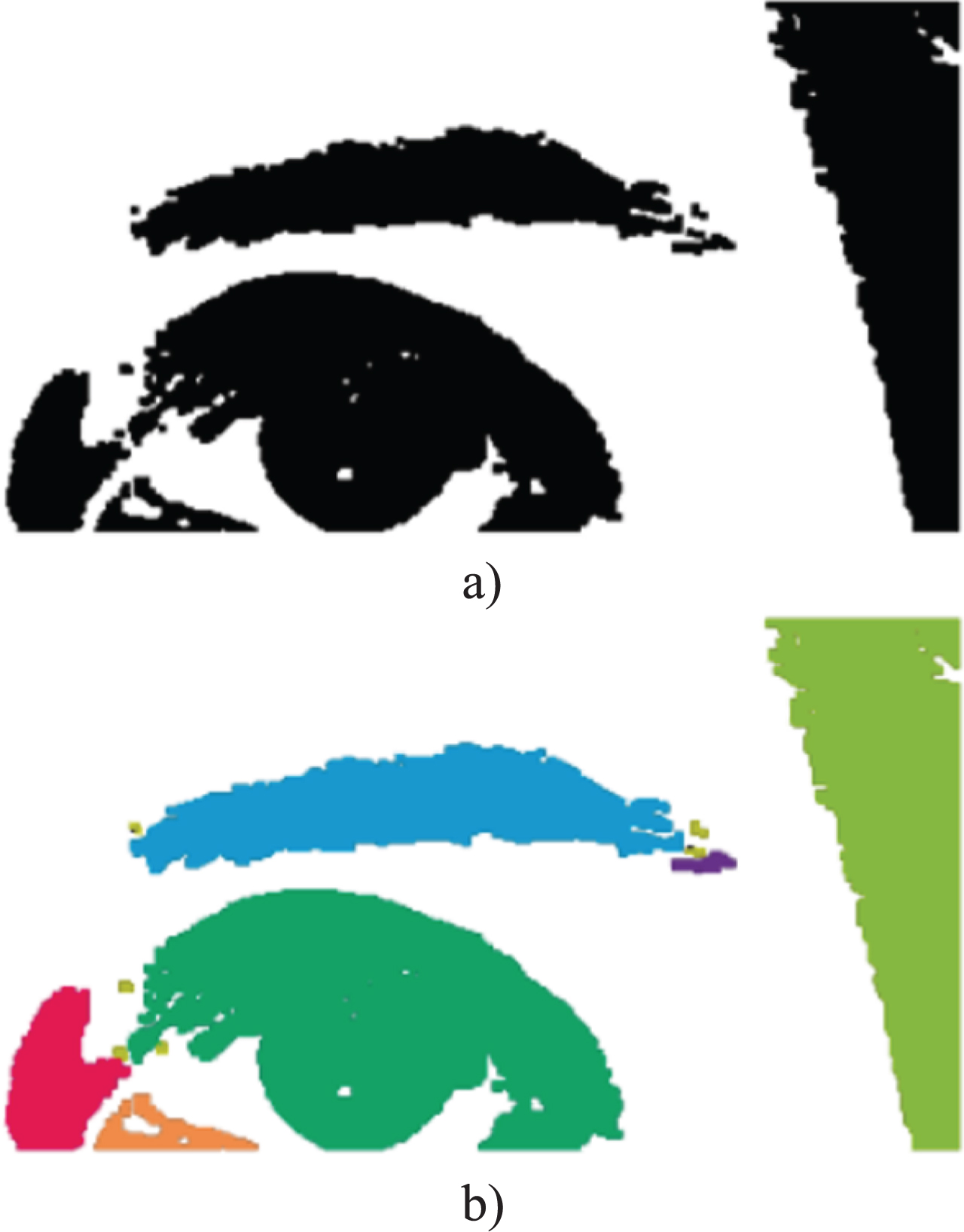
Example of dense region in a binary image.

Algorithm 2

Edge DEtection in Mouth (EDEM) algorithm.

Require : Image in RGB color model I

Binary image with mouth edges I_s

1: Separate intensity values of channels I=I_R, I_G, I_B

2: for each value in I_R and I_Bdo

3: G_V = Apply vertical gradient (Fig. 4a)

4: G_H = Apply horizontal gradient (Fig. 4b)

5: value =

\sqrt{(G_{V})^{2} + (G_{H})^{2}}

6: The new pixel value will be:

255 * Sin (\frac{π * value}{2 * 255})

7: end for

8: Compute the histogram (H_R, H_G) of each new image

9: Compute the mean of I related to the intensity values μ:

\frac{width * heigth}{255}

10: for each value in I_R and I_Bdo

11: if the frequency of the histogram value is minor than μthen

12: The new value of the pixel in I_s will be 255

13: end if

14: end for

15: Binarize I_s with threshold = 127

16: Return I_s

The proposed algorithm for detecting dense regions in binary images is shown in Algorithm 3 (DERBI, DEnse Region in Binary Images), in this process only black pixels are processed, the coordinates of each pixels in the image are listed, in the first step a cluster with the first point is created, then if their neighbors pixels are black these are added to the cluster, the added pixels are marked as visited, the neighbors pixels are analyzed with the same process. If all the pixels in the cluster are analyzed, a new pixel is choosen, the process finishes when all the black pixels in the image are analyzed. As output of the Algorithm 3 a list with the clusters is returned, then some metrics like black pixels with respect to the rectangular area of the cluster and width with respect to height are used to filter the ROI in the binary image.

Algorithm 3

DEnse Regions in Binary Image (DERBI) algorithm.

Require: Binary image I_s

Ensure: List with the clusters in I_s (Clusters)

1: A list with the points coordinates of the black pixels in I_s (Points)

2: for each point x in Pointsdo

3: ifx is not visited then

4: Create a cluster and add to Clusters

5: Add the coordinates to the current cluster with their neighbors in Points

6: Set the pixels coordinates as visited

7: for each value in the current cluster do

8: Add the neighbors coordinates to the current cluster of the not visited neighbours and then set as visited

9: end for

10: end if

11: end for

Return Clusters

3.2 Feature extraction

In the feature extraction stage, numerical values are extracted from the segmented regions in the pre-processing step. In feature extraction process, interpolated polynomials are used to get two sets of features (one with coefficients and other with points based on the polynomials), then these sets are tested in the classification process, in this section the approach to extract interpolated polynomials in eyebrows and mouth regions are presented.

For eyebrow region a polynomial of degree 3 is found, the polynomial of degree 3 is adjusted to the eyebrow region as can be seen in Fig. 6. Some columns in binary images are analyzed. For finding black pixels in a column a Δ value is used as an increment in order to not analyze all the columns. The average of all the positions of black pixels in a row is added to the Points set; then, four representative points according to the Fig. 6 are used to find a polynomial of degree 3 with the divided difference of Newton method. Finally, as output of the algorithm a polynomial of degree 3 is returned. This process can be seen as pseucode in Algorithm 4 (EPE, Eyebrow Polynomial Extraction).

Fig.6

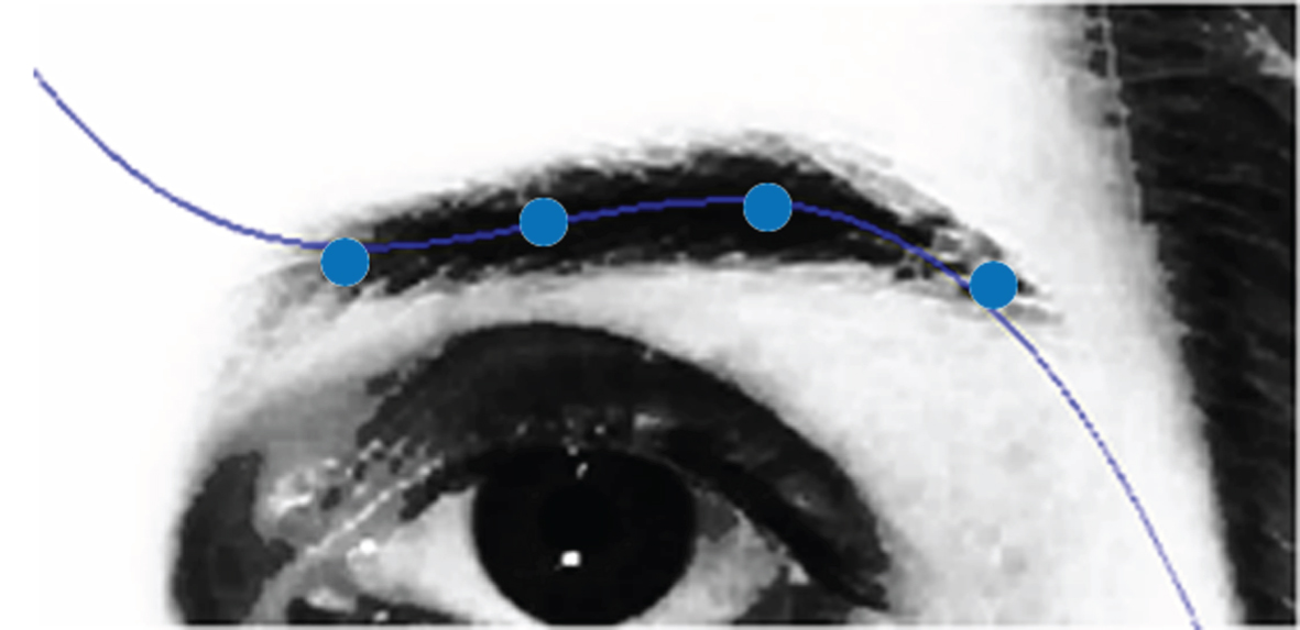
Polynomial of degree 3 in eyebrow region and representative points.

A similar process is applied in mouth region, for this region two polynomials of degree 2 are used as representative attributes (one for the upper part and other for the lower one) as can be seen in the Fig. 7. This process can be seen in the Algorithm 5 (MPE, Mouth Polynomial Extraction), the main difference between EPE and MPE algorithms is in line 5. Here, maximum and minimum points are found in order to obtain the two polynomials. As output of the algorithm two polynomials of degree 2 are extracted. In the next section these features will be evaluated with several supervised learners to obtain a model to classify new examples.

Fig.7

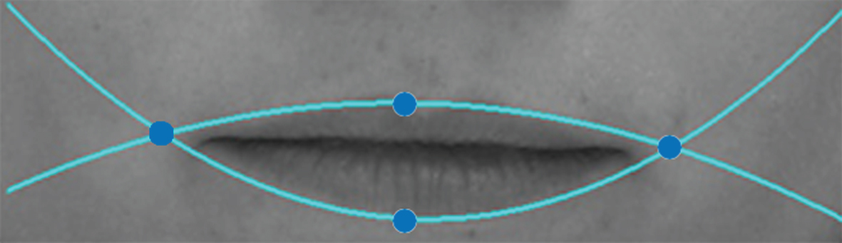
Polynomials of degree 2 in mouth region and representative points.

Algorithm 4

Eyebrow Polynomial Extraction (EPE).

Require: Binary image I, Δ

Ensure Polynomial of degree 3 (Polynomial)

1: List of Points (Points)

2: x = 0

3: whilex < number of rowsdo

4: Find the average of the columns number of the black pixels in row x (Av)

5: Add the point (Av, x) to Points

6: x = x + Δ

7: end while

8: Find a polynomial of degree 3 with the most representative points as can be seen in Fig. 6 (Polynomial)

9: Return Polynomial

3.3 Classification

In this stage, some supervised learners are tested in order to obtain a model with acceptable accuracy to classify new examples. For this case, three of the six universal emotions (happiness, surprise and anger) are classified using MMI dataset [13].

Learners, such as: K-NN, decision trees (C4.5) and Neural Networks with a feed-forward architecture with one hidden layer are tested in this stage. For NN classifier different parameters (momentum, learning rate and number of neurons in the hidden layer) are tested to obtain the highest accuracy. The experimental results are shown in Section 4.

Algorithm 5
Mouth Polynomial Extraction (MPE).

Require Binary image I, Δ

Ensure Two polynomials of degree 2 (MaxPolynomial and MinPolynomial)

List of maximum points (MaxPoints)

1: List of minimum points (MinPoints)

2: x = 0

3: x = 0

4: whilex < numberofrowsdo

5: Find the maximum (max) and minimum (min) black pixels in row x

6: Add (max, x) to MaxPoints

7: Add (min, x) to MinPoints

8: x = x + Δ

9: end while

10: Find a polynomial of degree 2 with the most representative points as can be seen in Fig. 7 for the lower and the upper parts of mouth regions (MaxPolynomials, MinPolynomials)

11: Return MaxPolynomial and MinPolynomial

In this section five algorithms are presented, in order to show the process of our approach a flowchart is depicted in Fig. 8. EDEM and ERED algorithms are applied for pre-processing stage, the output of this algorithms are the input of DERBI algorithm, the ROIs are filtered, then a binary image for each case is used as input of the EME and MPE algorithms for feature extraction process. Finally, two sets of features are extracted and are tested in classification stage.

Fig.8

Flowchart of algorithms processing.

4 Results

In this section results with different datasets for each stage of the proposed methodology are presented. For these results the used databases are:

MMI database, consists of 474 images captured from five subjects [13].

Jaffe database, contains 213 images from 60 subjects 7 expressions are taken into account [18].

VidTIMIT contains video and audio recording from 43 persons [19].

In segmentation process the MMI dataset is used for both mouth and eyebrow segmentation. Additionally, this database is used for classification stage. Jaffe and VidTIMIT are used for mouth segmentation. In the following sections the results for each stage are reported.

4.1 Pre-processing results

The results of ROIs segmentation (mouth and eyebrow) are presented in this section, an example of each segmentation with an image from MMI dataset can be seen in the Figs. 9 and 10 respectively. For both processes every step of the segmentation algorithm is shown.

Fig.9

Example of eyebrow segmentation: a) Input image; b) Hyperbolic tangent filter; c) Filter of Equation 1; d) Otsu binarization algorithm; e) DERBI algorithm.

Fig.10

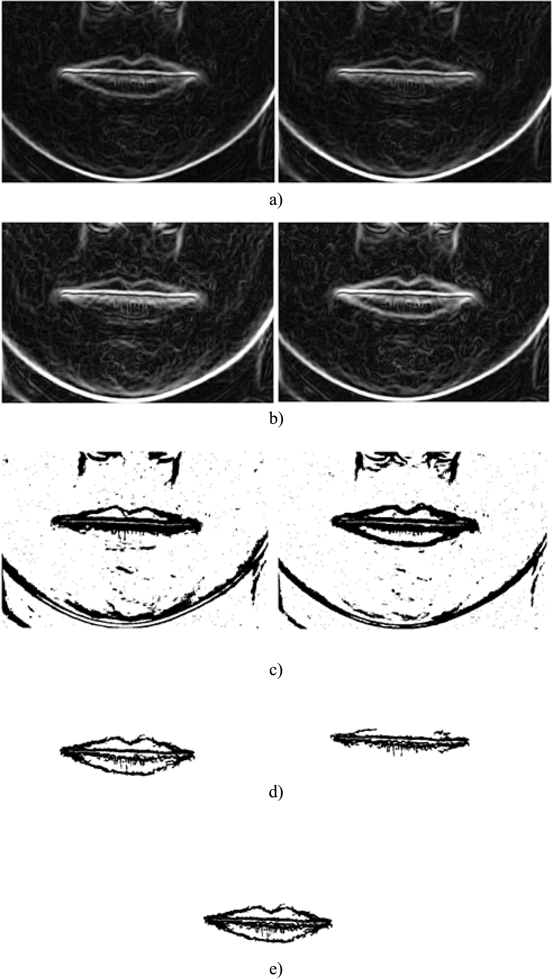
Example of mouth segmentation: a) Gradient filter in two directions; b) Sine filter; c) denoised image based on mean; d) application of DERBI algorithm; e) XOR function.

In order to show the results of segmentation and feature extraction process, ERED and EDEM algorithms results with MMI database are shown in Fig. 11. In this figure, the segmentation of the proposed approach for ROIs segmentation are marked in white color. For eyebrow case the full region is segmented. On the other hand, the border of mouth region is extracted.

Fig.11

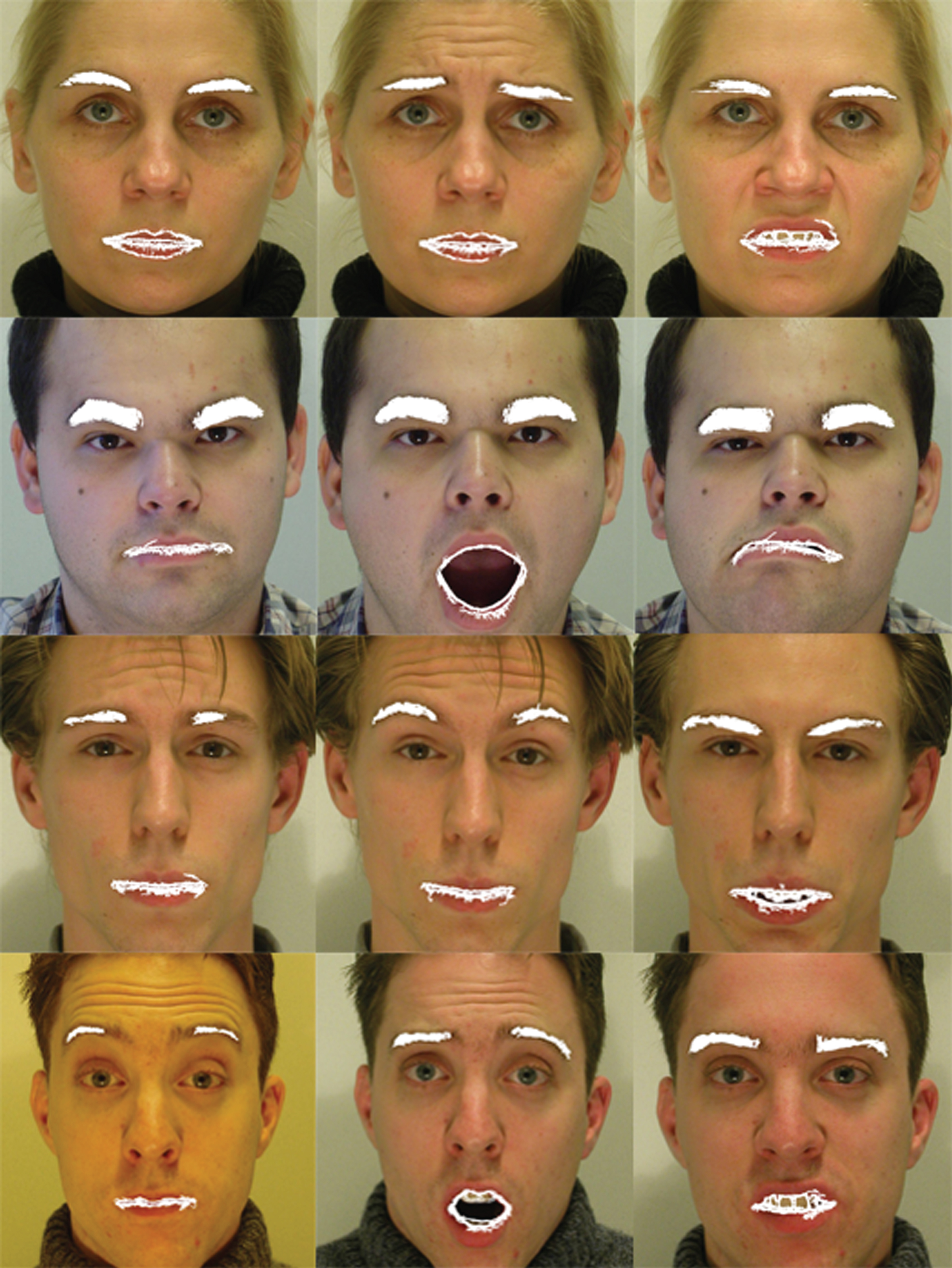
Results of mouth an eyebrow segmentation with MMI dataset.

For the feature extraction approach the Jaffe and VidTIMIT datasets are used, before applying the pre-processing approach smoothing and automatic contrast adjustment filters are applied. The results of mouth segmentation with the feature extraction process of two datasets can be seen in Fig. 12 (for Jaffe dataset) and Fig. 13 (for VidTIMIT dataset). The results of the feature extraction process are marked in white color.

Fig.12

Results of mouth segmentation with Jaffe dataset.

Fig.13

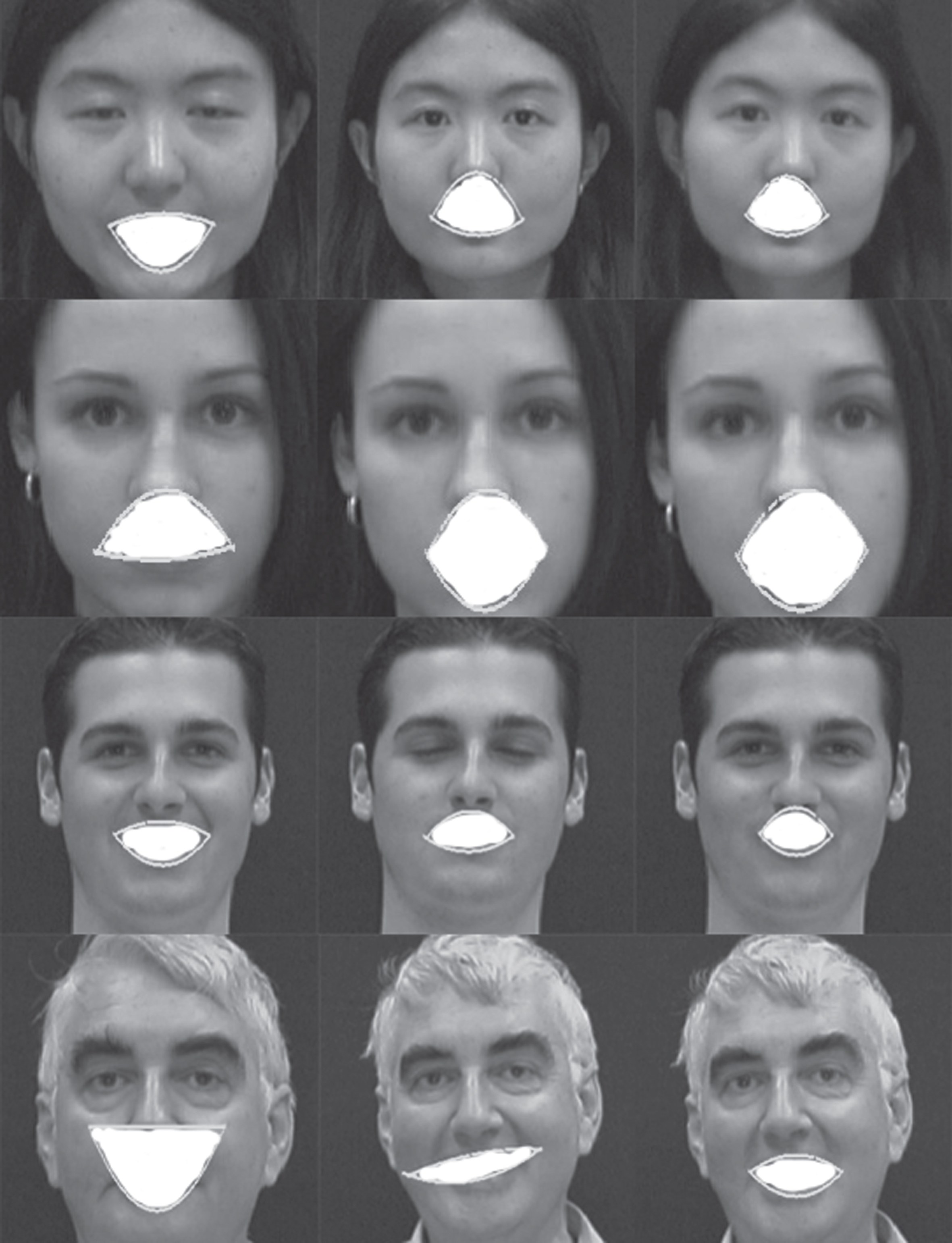
Results of mouth segmentation with VidTIMIT dataset.

A control set with the borders of mouth regions and eyebrow region is used to compare the obtained coefficients for the regions, the control set consists of 5 images of some subjects from MMI dataset, then the coefficients of the control set and segmented images with our approach are compared, making a difference between the coefficients and getting the mean and standard deviation of these differences. The lower mean and standard deviation values the better segmentation result, the results of the comparison can be seen in the Fig. 14 (for mean results) and 15 (for standard deviation results). As can be seen, values are near to zero, for this reason, our segmentation process have an acceptable performance.

Fig.14

Mean of the error in the comparison of the polynomials of mouth and eyebrow regions.

Fig.15

Standard deviation of the error in the comparison of the polynomials in mouth and eyebrow regions.

4.2 Classification

In classification process the MMI dataset is used. We test different supervised learners for numerical values such as: K-NN, decision trees, and NN which are trained with two sets of features: one for with the coefficients (Coefficients Features, CF), and other with ten points extracted from each polynomial (Points Features, PF). The training set consist of 42 instances for happiness, 17 for anger and 20 for surprise (H, A, S respectively). In all the experiments 5-fold-cross-validation is used, the attributes are normalized via z-score method.

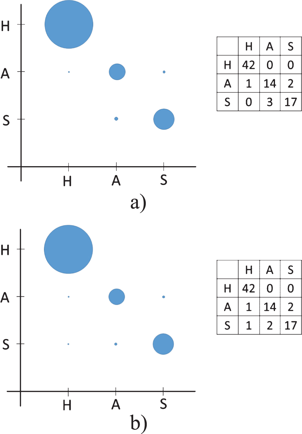
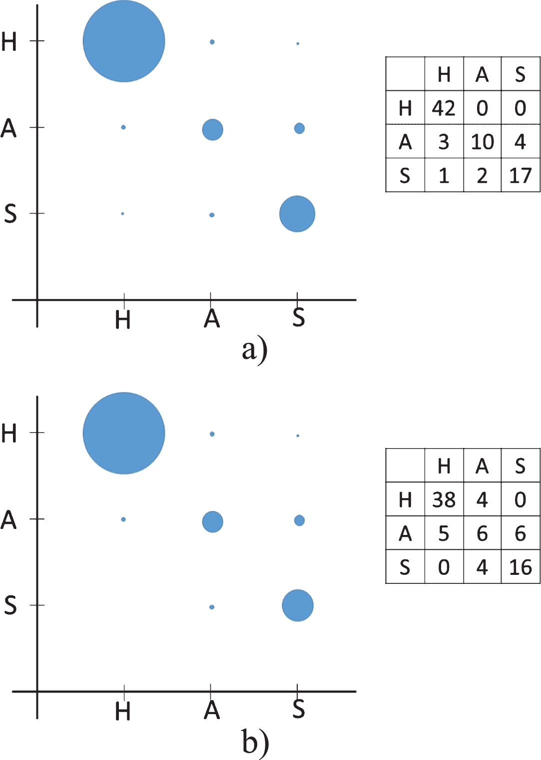
Our first experiments are applied with NN classifier, for all experiments a feed forward architecture is used with one hidden layer, then parameters such as: momentum, learning rate and neurons in the hidden layer are changed in order to obtain an acceptable accuracy. For PF set, some experimented paramenters are shown in Table 1. The highest accuracy are marked in bold, there is a difference in the confusion matrix of the two best parameters that can be seen in the Fig. 16 with their dispersion graph (the radius of the circle represents the number of instances classified) in Fig. 16a some surprise instances are confused with Anger, on the other hand in Fig. 16b surprise instances are confused with happiness and anger, both experiments have the same accuracy of 92.4%.

Fig.16

Confusion matrices and dispersion graphs of NN with PF: a) row 1 of Table 1 b) row 2 of Table 1.

Table 1

Some experimented parameters with NN and PF set

Epochs	Neurons in hidden layer	Momentum	Learning rate	Accuracy
500	39	0.3	0.06	92.4%
500	44	0.4	0.06	92.4%
500	41	0.1	0.27	91.8%
1000	45	0.16	0.58	91.3%
1500	45	0.11	0.06	91.9%

The CF set is tested with NN classifier as a similar way of PF set. In Table 2 the best experimented parameters for the CF set are shown. The confusion matrix and dispersion graph of the two best parameters of Table 2 can be seen in Fig. 17. These results have lower accuracy than experiments with PF set, we need to take into account that polynomials are extracted by Newton divided differences method.

Table 2

Some experimented parameters with NN and CF set

Epochs	Neurons in hidden layer	Momentum	Learning rate	Accuracy
500	41	0.01	0.11	83.54%
500	36	0.13	0.04	82.53%
1000	36	0.14	0.04	84.81%
1000	45	0.39	0.08	79.74%
1500	35	0.18	0.15	78.48%

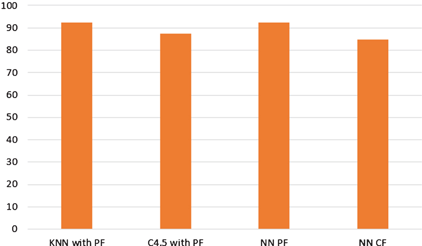
Other tested learners are decision trees and K-NN. In the experiments for K-NN K = 1 is used, for higher value of the K parameter, the classification accuracy is lower (seen Table 3). In Fig. 18 the confusion matrices and dispersion graphs are depicted (Fig. 18a has PF as input, 18b has CF as input). Note that the best classification is when PF is used as input of the learner. In addition, we obtain the same accuracy as NN learner (92.4%). There exists a difference in the confusion matrix, in NN anger is confused in one example with happiness and two examples with surprise, while in KNN case anger is confused in one instance with surprise and two instances for happiness.

Fig.17

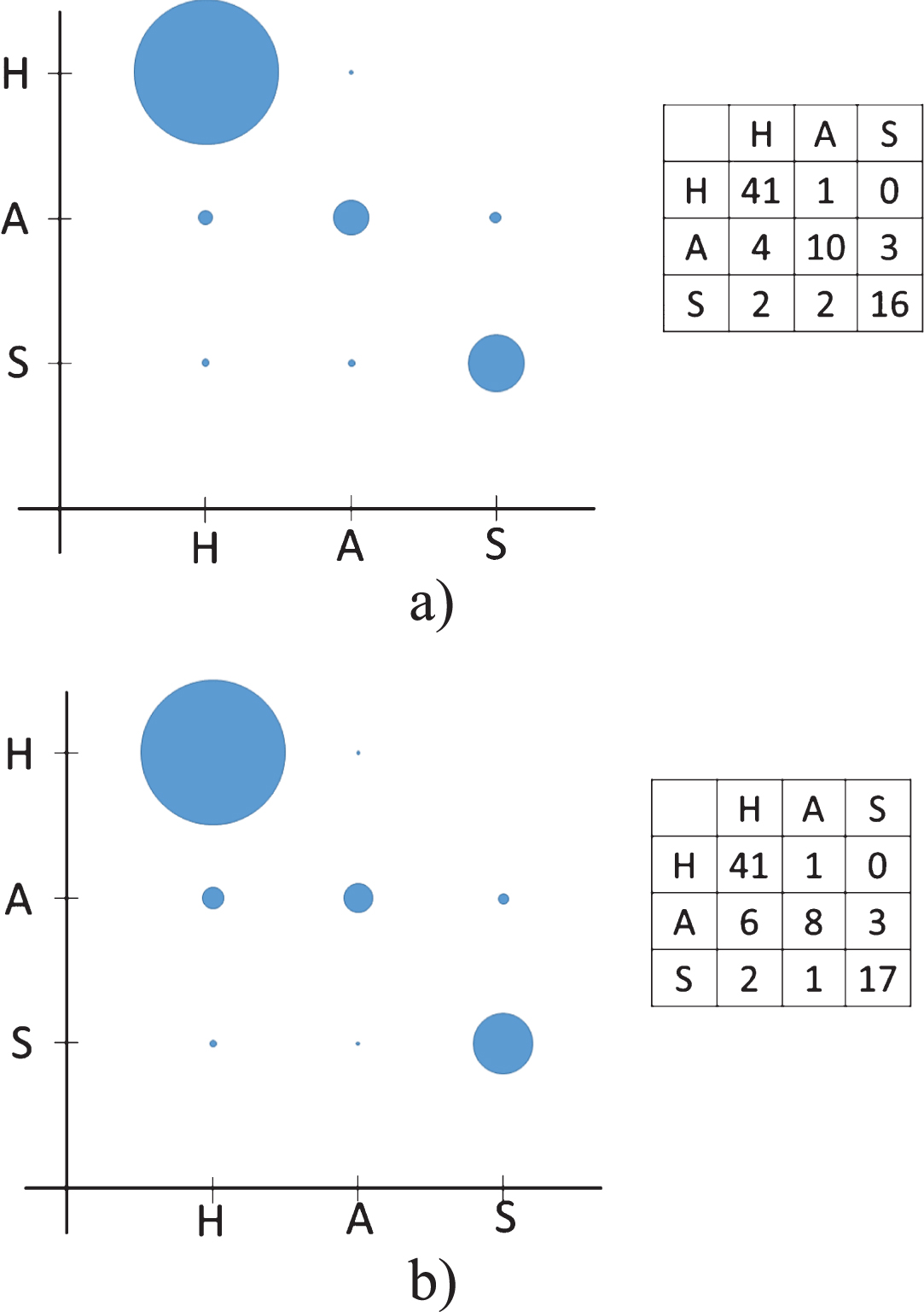
Confusion matrices and dispersion graphs of NN with CF: a) row 3 of Table 2 b) row 1 of Table 17.

Fig.18

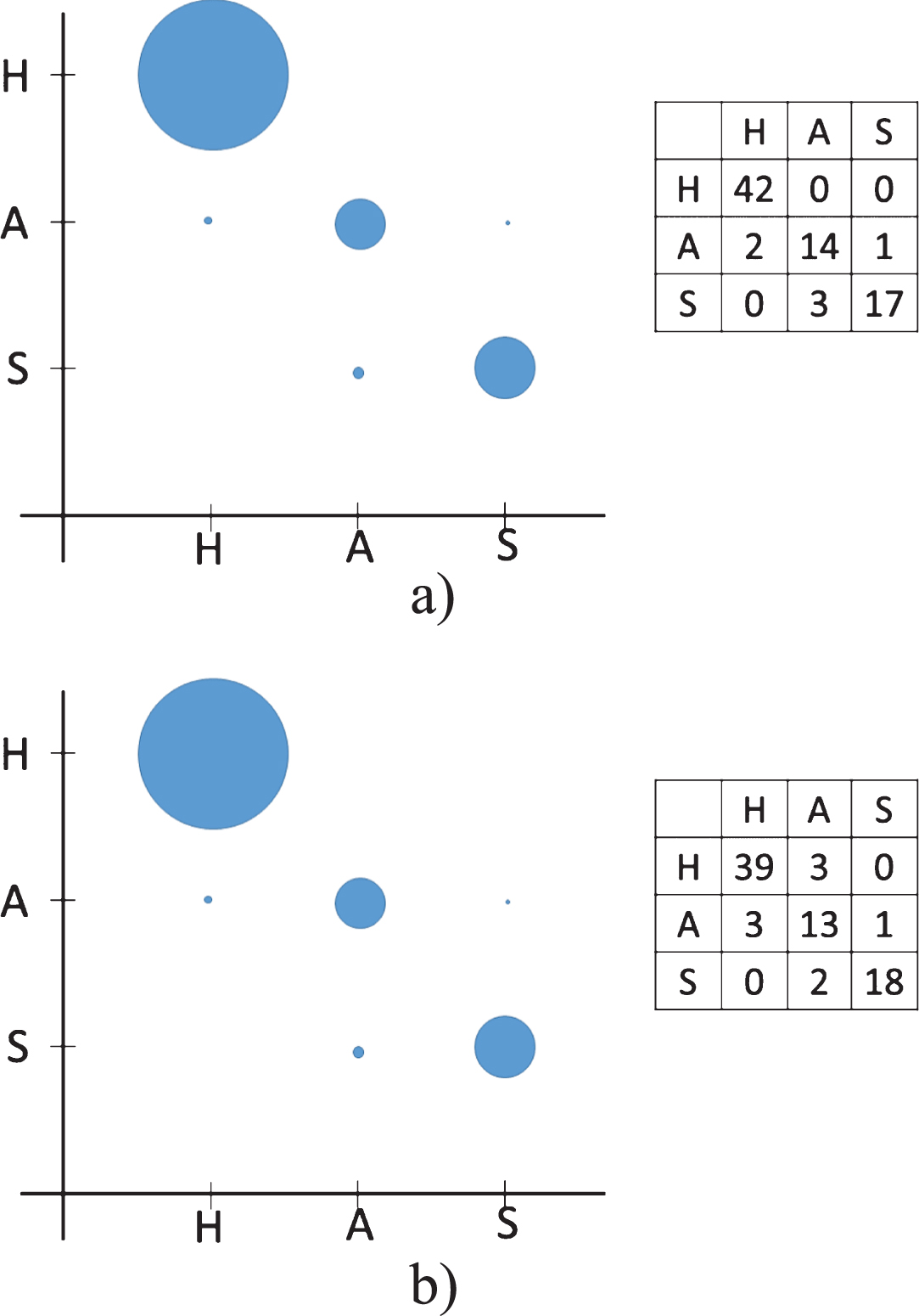
Confusion matrices and dispersion graphs of KNN: a) PF as input; b) CF as input.

Table 3

Experimented values for K-NN classifier

PF set		CF set
K value	Accuracy	K value	Accuracy
1	92.40%	1	88.60%
2	83.54%	2	78.48%
3	82.27%	3	79.74%
4	81.01%	4	81.01%

Decision trees C4.5 are used considering a confidence factor with 0.25 value and taken into account one as the minimum value of instances per leaf. In Fig. 19 the confusion matrices and dispersion graphs are shown: a) having PF as input; b) having CF as input. The best accuracy for decision trees case is when PF set is used as input with 87.34%, this classifier have the worst accuracy of the tested learners.

Fig.19

Confusion matrices and dispersion graphs of Decision trees: a) PF as input; b) CF as input.

As a graphical way to see the results of the learners accuracy, a histogram with the best accuracies are depicted in the Fig. 20, as can be seen, NN classifier when PF is used as input, the same case of KNN with K = 1, that have a same accuracy (92.4%) but different confusion matrix, the advantage of KNN is that training process is faster than the parameters adjustment of NN, decision tree C4.5 have a good performance for detecting happiness instances as can be seen in the confusion matrix (Fig. 19).

Fig.20

Best accuracy histogram for tested learners.

5 Conclusions and future work

In this work a methodology for emotion recognition based on interpolation polynomials features is presented. In pre-processing stage a process for eyebrow and mouth segmentation is introduced, here thresholding techniques and edge detector are improved in order to obtain a segmentation of the ROIs. Additionally, a method based on dbscan is proposed for detecting clusters in binary images, then different metrics such as density and width respect height are used to filter the ROIs.

For feature extraction, two sets of numeric values using interpolated polynomials that are found via divided differences of Newton Method are extracted. One set of features consist of coefficients of the polynomials and the other set contains points found with the polynomials, this sets of features are evaluated in classification stage.

In classification process learners such as NN, KNN and Decision trees are tested in order to obtain the best model to evaluate new examples, for NN different parameters are tested, in general PF set has the best performance in classification process, NN and KNN with K = 1 obtain the best accuracy in our experiments (92.4%).

As future work, more features of other ROIs will be extracted in order to improve the accuracy performance. A classification taking into account the six basic emotions and neutral state will be applied. A bigger set of features will be tested applying our approach. Finally, a dataset with the six basic emotion will be captured, obtaining spontaneous reaction of the subjects.

Footnotes

Acknowledgments

We thank the anonymous reviewers for their valuable comments. The first author thanks the support by the CONACyT Mastering Scholarship 701191.

References

Ekman

, Strong evidence for universals in facial expressions: A reply to Russell’s mistaken critique, Psychological Bulletin115(2) (1994), 268–287.

Cohn

, Ambadar

and Ekman

, in The handbook of emotion elicitation and assessment, Coan

& Allen

JJB

, Editors, Observer-based measurement of facial expression with the Facial Action Coding System (2007), pp 203–221.

Wen

, Hou

, Li

, Jiang

and Xun

, Ensemble of deep neural networks with probability-based fusion for facial expression recognition, Cognitive Computation (2017), 1–14.

Sonmez

E.B.

and Cangelosi

, Convolutional neural networks with balanced batches for facial expressions recognition, Proceedings of Ninth International Conference on Machine Vision, 2017.

Liu

, Han

, Meng

and Tong

, Facial expression recognition via a boosted deep belief network, Proceedings of IEEE Conference on Computer Vision and Pattern Recognition, 2014.

Xiaoming

and Wushan

, Facial expression recognition based on edge detection, International Journal of Computer Science & Engineering6(2) (2015), 1–9.

Ashir

A.M.

and Eleyan

, Facial expression recognition based on image pyramid and single-branch decision tree, Signal, Image and Video Processing11(1017) (2017), 1–8.

Happy

S.L.

and Routray

, Automatic facial expression recognition using features of salient facial patches, IEEE transactions on Affective Computing6(1) (2015), 1–12.

Siddiqi

M.H.

, Alam

M.G.

, Hong

C.S.

and Khan

A.M.

, and Choo

, A novel maximum entropy markov model for human facial expression recognition, PLoS ONE11(9) (2016), 14–23.

10.

Sabu

, Geometrical model of facial regions and CUDA based parallel face segmentation for emotion recognition, International Journal of Applied Engineering Research11(9) (2016), 6740–6752.

11.

Rahulamathavan

, Phan

R.C.

, Chambers

J.A.

and Parish

D.J.

, Facial expression recognition in the encrypted domain based on local fisher discriminant analysis, IEEE Transactions on Affective Computing4(1) (2013), 83–92.

12.

Pell

M.D.

and Kotz

S.A.

, On the time course of vocal emotion recognition, PLoS ONE6(11) (2011), 1–16.

13.

Pantic

, Valstar

, Rademarker

and Maat

, Web-based database for facial expression Analysis, Proceedings of International Conference on Multimedia and Expo2005.

14.

Viola

and Jones

, Rapid Object Detection using a Boosted Cascade of Simple Features, Proceedings of Computer Vision and Pattern Recognition2001.

15.

Otsu

, A threshold selection method from gray-level histogram, IEEE Transaction on Systems, Man, and Cibernetics9(1) (1979), 62–66.

16.

Ester

, Kriegel

H.P.

, Sander

and Xu

, A density-based algorithm for discovering clusters in large spatial databases with noise, KDD96(34) (1996), 226–231.

17.

Atkinson

, An introduction to numerical analysis, John Wiley & Sons2008.

18.

Michael

, Shigeru

, Miyuki

and Jiro

, Coding Facial Expressions with Gabor Wavelets, Proceedings of International Conference on Automatic Face and Gesture Recognition1998.

19.

Conrad

and Brian

,Multi-region probabilistic histograms for robust and scalable identity inference, Lecture Notes in Computer Science (LNCS)5558 (2009), 199–208.