Feature engineering based on ANOVA,cluster validity assessment and KNN for fault diagnosis in bearings

Abstract

The number of features for fault diagnosis in rotating machinery can be large due to the different available signals containing useful information. From an extensive set of available features, some of them are more adequate than other ones, to classify properly certain fault modes. The classic approach for feature selection aims at ranking the set of original features; nevertheless, in feature selection, it has been recognized that a set of best individually features does not necessarily lead to good classification. This paper proposes a framework for feature engineering to identify the set of features which can yield proper clusters of data. First, the framework uses ANOVA combined with Tukey’s test for ranking the significant features individually; next, a further analysis based on inter-cluster and intra-cluster distances is accomplished to rank subsets of significant features previously identified. Our contribution aims at discovering the subset of features that discriminates better the clusters of data associated to several faulty conditions of the mechanical devices, to build more robust multi-fault classifiers. Fault severity classification in rolling bearings is studied to verify the proposed framework, with data collected from a test bed under real conditions of speed and load on the rotating device.

Keywords

Feature engineering ANOVA cluster validity assessment KNN fault diagnosis bearings

1 Introduction

There are constant increasing requirements for the continuous working of the transmission machines. This is why new approaches to build fault diagnostic systems with accuracy and reliability are highly valuable. Alternative computational approaches using Machine Learning (ML) for fault diagnosis have been developed by using Neural Networks [2, 25], Support Vectors Machines [39], Cluster Analysis [19] and Decision Trees [4]. These ML approaches have been very useful for implementing condition-based maintenance, as presented in [3, 15]. In case of ML-based fault diagnosis in mechanical rotating machinery, a sizable amount of features could be extracted from different signals which are processed to obtain condition parameters in time, frequency and time-frequency domain. There exist a wide set of alternatives to build robust classifiers, such as those based on decision trees and deep learning architectures, for which the number of input features does not decrease their performance [1 , 16–18]. In the framework of the supervised feature selection, feature analysis is widely applied to select the most significant features improving the accuracy of machine learning based diagnostic models [2 , 36], and more recently into a unsupervised manner [24].

Beyond the availability of complex robust ML models that can deal with a high dimensional feature space, the identification of the most significant features contributes to discover relevant knowledge about the application problem, at the same time that such features can lead to build more simple and also robust ML models, usually easier to interpret. Feature engineering arises as an essential topic in ML to identify features that are useful to build optimized models for explanation or for accuracy, from two perspectives of analysis, respectively: feature relevance and feature selection. Some works consider the analysis of the feature relevance as part of the feature selection process. Feature selection is a NP-hard problem, and several approximation algorithms have been proposed to find the near best feature subset over a reasonable time [5, 11]. Besides the most common metrics to measure the feature relevance, such as Gini Index, Information Gain, and Mutual Information (MI), statistic tests such as Chi-square and Analysis of Variance (ANOVA) can be used to measure relevant features regarding a set of class labels. They are very used for feature selection in text mining, emotion recognition, bioinformatics and medicine. However, its use in engineering applications to fault diagnosis is not widely reported.

This work is focused on both feature relevance and feature selection. Specifically, this paper proposes a supervised methodological framework for feature analysis using ANOVA and a cluster distance metric. In the first step, ANOVA is used to rank individually the statistical relevance of the features; in the second step, a cluster validity assessment index is used to rank the subsets of features that yield better cluster structures related to the failure modes, i.e. classes, under study. As result, a subset of features is identified, which reflects the discriminative information regarding the different classes. Previous works show ANOVA as powerful statistic test widely used to rank the feature relevance in supervised classification. Particularly, we are motivated in using ANOVA due to its ability to identify features discriminating set of data regarding the mean value, and this is considered a first step for selecting features that yield adequate cluster structures. ANOVA combined with other metrics to measure the ability of the relevant features to create proper clusters for classification is not studied, and this is our main contribution. A real dataset for fault diagnosis in bearings is evaluated to test our framework. Comparisons to the cluster structure obtained from the classic feature selection and reduction techniques are provided in order to show the performance of our algorithm. Finally, a K-Nearest-Neighbours (KNN) based supervised classifier is used to assess the performance of the selected features to give a proper fault diagnosis. Comparison to features selected by the Random Forest(RF) algorithm is also provided.

The following sections are organized as follows. Section 2 discusses some works related to feature selection preserving cluster structures, and related techniques to our proposal. Section 3 presents the theory used in this work. Section 4 introduces the proposed methodological framework for feature selection by using ANOVA and cluster validity assessment. Section 5 presents the results obtained with the proposed approach, and some analysis are developed. Finally Section 6 concludes the paper.

2 Related works

There are several works discussing the problem of feature selection for clustering from unsupervised or supervised manner. Compactness and separation measures are considered in [6], to quantify features that ensure the proper intra and inter cluster scatters. More recently, some works aim at preserving the cluster structure of the samples composing the dataset. In [34], an unsupervised feature selection method using a group sparse feature selection on local learning based clustering is proposed. In [7] a feature selection based on Mutual Information is developed to identify salient features, that are useful for maintaining the nearest and farthest neighbours from an instance, or sample. In [28], spectral clustering is introduced to discover the cluster structure and discriminative analysis between features is used to preserve the structure. In [21], the feature selection is based on the idea of minimizing the violation of the initial cluster structure and penalizing the use of features. Other approaches for feature selection are proposed into supervised environments, where MI is the main index used to rank features [20]. Recently, [32] proposes the use of a self-similarity factor as indicator to measure the feature importance into an affinity propagation based clustering process.

With regard to the use of ANOVA, it is reported for feature selection in classification of data related to gas chromatography [27, 31]. In [14], the performance of the selected features by using ANOVA is tested regarding their ability to yield proper clusters after applying feature reduction with Principal Component Analysis on data related to chromatographic features relevant to a given classification of jet fuels. ANOVA has been also reported as technique for feature relevance analysis in other types of industrial devices. In [9], ANOVA is performed over data obtained from the stator current of an induction motor, where different fault conditions are simulated by a progressively hole drilling into a rotor bar. In [10], multivariate ANOVA is applied for feature selection in internal combustion engine valve clearance fault classification; next, the Wilks statistic is used to determine the class separation ability of other feature combined with the previous selected ones. In [30], ANOVA is applied to determine the effect of each individual parameter of the stator winding fault model response, for running the induction motor with the best parameter values in its parameters range. The effect of different valve conditions on the Root Mean Square (RMS) value at its corresponding time-frequency segments, extracted from the acoustic emission signals, are analysed by using ANOVA in [29].

In the field of fault diagnosis of rotating machinery, the vibration signatures are analysed by one-way ANOVA method in [37] to conclude that a faulty state can be identified from the healthy one, but some faulty states cannot distinguish between them. In [12], two stage feature selection through ANOVA and a weighting technique is used to diagnose the gear crack development. In [38] ANOVA is applied to select the most relevant principal components to diagnose faults in a multi-shaft centrifugal compressor. In [22] ANOVA is used for analysing the main effects of the rotational speed and the radial load on the mean and standard deviation of the acoustic signal measured in dry and lubricated bearings. In [8] ANOVA was used to determine influence of the blade vibratory amplitude, the signal-to-noise ratio, the sampling time, and the sampling frequency on the side-band and noise amplitudes in the frequency domain of the vibration signal. ANOVA test was conducted in [35], in order to check the statistical significance of the gear fault separation by using RMS time synchronous average.

3 Background

3.1 Analysis of Variance (ANOVA) and Tukey’s test

ANOVA is a powerful statistical test to reject the null hypothesis H₀ stated as H₀ : μ₁ = μ₂ = … = μ_K, where μ_i, i = 1, …, K are the means of the K different data population, under assumption of the population independence, normality and homoscedasticity [23]. However, ANOVA can works well enough even under slight assumption violations. The alternative hypothesis H_a states that H_a : μ_i ≠ μ_j for some i, j s.t. i ≠ j, j ≤ i. Each population, i.e. continuous values of the response variable Y, is characterized by one or more categorical factor, then ANOVA compares the means of the response variable into the different factors levels. One-way ANOVA only considers one factor with two or more levels (or groups). To accept H₀ in one way ANOVA, the F-test is used by computing the F-statistics given by Equation (1): $F = \frac{\frac{\underset{i = 1}{K \sum} n_{i} {({\bar{Y}}_{i} - \bar{Y})}^{2}}{K - 1}}{\frac{\underset{i = 1}{K \sum} \underset{j = 1}{n_{i} \sum} {({\bar{Y}}_{ij} - {\bar{Y}}_{i})}^{2}}{N - K}}$ (1) where $\bar{Y_{i}}$ denotes the sample mean in the i-th group, n_i is the number of samples in the i-th group, $\bar{Y}$ denotes the overall mean of the samples, Y_ij is the j-th sample in the i-th group, and K denotes the number of groups.

The F-value is expected to be approximately 1 under H₀, however to reject H₀, a high F-value is needed. A single high F-value is hard to interpret on its own. Then, the reference value to reject H₀ is based on the p-value, which is the probability of observing a F-value that is at least as high as the value that our study obtained, under the assumption that H₀ is true. Commonly, H₀ is rejected if p ≤ 0.05. Once the ANOVA test rejects the null hypothesis, multiple comparison by using the Tukey’s test is required to identify any difference between two means μ_i - μ_j, by calculating the ratio in Equation (2): $q_{s} = \frac{μ_{i} - μ_{j}}{{SE}_{\bar{x}}}, μ_{i} - μ_{j} > 0$ (2) where ${SE}_{\bar{x}}$ is the expected standard error of the mean. The q_s value is compared to the q critical value from the studentized range distribution. If q_s is larger than the q critical value obtained from the distribution, the two means are significantly different. The distribution of q and its critical values have been tabulated and available to pairwise comparison.

3.2 Clustering validity assessment

In some applications of supervised classification, the cluster structure of a dataset could be an interesting information to select the proper features addressing better classifiers. In this work, an overall clustering validity index, called Composing Density Between and With clusters (CDbw), is used to measure the cluster structure [13, 33]. This index puts emphasis on the geometric characteristics of clusters, such as compactness and separation. According to [13], a cluster i is composed by n_i samples $x \in ℝ^{n}$ and, besides the centroid (mean point of the cluster), there are r_i fixed representatives points v_{ir
_i} which are generated in an iterative procedure. In the first iteration, the point farthest from the centroid is chosen as the first representative point. The next representative point is chosen such that it is farthest from the previously chosen point, and so on.

Given a cluster partition, instead of using only distance information, intra-cluster and inter-cluster density information are also considering by the index CDbw, as stated in Equation (3): $CDbw (c) = Intra_D (c) Sep (c)$ (3) where c is the number of cluster in the partition, Sep (c) measures the separation between clusters and Intra _ D (c) measures the intra-cluster density.

On one hand, Sep (c) in (3) considers both the inter-cluster distances and the inter-cluster density, as proposed in Equation (4): $Sep (c) = \underset{i = 1}{c \sum} \underset{j \neq i}{j = 1 c \sum} \frac{C_R (i) - C_R (j)}{1 + Inter_D (c)}, c > 1$ (4) where C _ R (i) and C _ R (j) are the closest pair of representations of two neighbour clusters i and j, and Inter _ D (c) measures the inter-cluster density defined as the density in the between-cluster areas. Inter _ D (c) is defined in Equation (5):

$\begin{matrix} Inter_D (c) \\ = \underset{i = 1}{c \sum} \underset{j \neq i}{j = 1 c \sum} \frac{C_R (i) - C_R (j)}{sd (i) + sd (j)} d (u_{ij}), c > 1 \end{matrix}$ (5) where u_ij is the middle point between the pair (C _ R (i) , C _ R (j)), sd (·) is the standard deviation vector of a cluster, and d (u_ij) = oversetn_i + n_j∑_i=1f (x_k, u_ij) is a density, n_i and n_j are the number of samples belonging to clusters i and j, respectively, and x_k is a data point of the clusters. The function f (x_k, u_ij) is defined by Equation (6): $f (x_{k}, u_{ij}) = {\begin{matrix} 1 & if x_{k}, u_{ij} \leq \frac{sd (i) + sd (j)}{c} \\ 0 & otherwise \end{matrix}$ (6)

On the other hand, Intra _ D (c) in (3) is defined as the number of points belonging to the neighbourhood of representative points of the clusters, as proposed in Equation (7): $Intra_D (c) = \frac{1}{c} \underset{i = 1}{c \sum} \underset{j = 1}{r_{i} \sum} Den (v_{ij}), c > 1$ (7) where r_i is the number of representatives points of the ith cluster, and Den (v_ij) = oversetn_i∑_l=1f (x_l, v_ij) is a density, x_l is a sample belonging to the ith cluster, v_ij is the jth representative point of the ith cluster; f (x_l, v_ij) is given by Equation (8): $f (x_{k}, u_{ij}) = {\begin{matrix} 1 & if x_{l}, v_{ij} \leq {sd}_{a} \\ 0 & otherwise \end{matrix}$ (8) where sd_a is the average of the standard deviation of all standard deviation vectors sd associated with each cluster.

The intra-cluster density and separation will be significantly high for well-separated clusters, then we use this metric to evaluate the obtained cluster structure when a subset of significant features is selected. More details about this metric can be found in [33].

4 Methological framework using ANOVA and Cluster Validity Assesment

In feature selection, it has been recognized that the combination of individually good features does not necessarily lead to good classification [26]. In this sense, feature selection performed in a way of individually feature ranking instead of globally one, is not considered as the best way to choose the more significant features. By using the p-value in the ranking process through ANOVA, several features can have very close value, or even some subsets of the relevant features discriminate better the fault classes than other subsets with the same best p-value. Then, further analysis after applying ANOVA might be oriented to a new ranking according to the cluster structure associated with the relevant features.

Our feature analysis includes a further analysis of the relevant features ranked by ANOVA, by using the cluster distance metric described in Section 3.2, applied to the clusters that have been created from the relevant features. This is with the aim of identifying the features that better discriminate certain fault modes. In this sense, several subset of features can be selected as input to a classifier dedicated to particular failures modes. This is specially useful for designing multi classifiers in real time industrial applications where noise and disturbances make the classification a sensitive task that could not be easily to solve with one centralized classifier. Of course, an exhaustive search must be developed to find the final subset of features; then, the feature selection might be formalized as a combinational optimization problem finding a feature set to maximize the quality of the hypothesis learned from these features. However, our work is not focussed on the searching algorithm but in the features analysis.

Let F, P and S be the sets of features, fault classes, and dataset, respectively, such that F = {f_j}, j = 1, . . . , n, P = {P_i}, i = 1, . . . , c, S = {(x^k, y^k)}, k = 1, . . . , m, $x^{k} \in ℝ^{n}$ is a vector of features and y^k is a categorical variable, y^k ∈ P. In the first stage, the methodological framework executes the classical ANOVA test followed by the Tukey’s test for a pairwise multi-comparison, to rank the most significant features. Due to several features can have a p-value p < 0.05 to reject the null hypothesis ANOVA, a threshold significance Th_s is set to select a feature f_j such that p_j < Th_s < 0.05. For each significant feature f_j, the Tukey’s test is applied and a threshold pairwise significance Th_{PW
_s} is set to finally select a significant feature ${\hat{f}}_{j}$ such that ${\hat{p}}_{j} < {Th}_{{PW}_{s}} < 0.05$ . Significance thresholds are chosen as a proportion over the maximum p-value, to avoid the empty set of the selected features. As result, several sets F_{Psp′_i} ⊂ F of significant features are obtained for each pair Psp′_i = (P_r, P_s) under study. This first analysis is repeated several times over sets Ssp′ ⊂ S composed by q samples randomly selected from the dataset S, q < m, in order to have a statistical significance. In our case, those features $\hat{f_{j}} \in F_{P'_{i}}$ that appear all the times, for all pairs, are kept for analysis in the next stage. Then, the set F_P of final significant features is obtained. For purposes of further analysis, the features in the set F_P are ranked in ascendant order according to Equation (9): $S_{f_{j}} = i \sum {\hat{p}}_{j}^{i}$ (9)

where S_{f
_j} denotes the feature ranking index, and ${\hat{p}}_{j}^{i}$ denote the ${\hat{p}}_{j}$ -value of the feature j in the set F_{Psp′_i}.

In the second stage, a set of classes $\hat{P} \subseteq P$ is defined for further analysis. Let $\tilde{F}$ be a set of all possible n-tuple of features in F_P, $\tilde{F} = {\tilde{f_{z}}}$ . The cluster structure for each pair $\hat{P}'_{i} = {P_{r}, P_{s}}$ , $P_{r}, P_{s} \in \hat{P}$ regarding the n-tuple $\tilde{f_{z}}$ is measured through the index ${CDbw}_{i}^{z}$ , as described in Section 3.2. The final cluster metric CDbwF_z, regarding $\hat{P}$ and $\tilde{f_{z}}$ is computed with Equation (10): ${CDbwF}_{z} = \frac{i \prod {CDbw}_{i}^{z}}{i \sum {CDbw}_{i}^{z}}$ (10)

Finally, the n-tuple of the most significant features f_best creating an adequate cluster structure for the set $\hat{P}$ is selected according to condition in Equation (11): $f_{best} = \tilde{f_{z}} s . t {CDbwF}_{z} is maximun$ (11)

Algorithms 1 and 2 show the pseudo-code to execute our methodological framework for feature analysis.

Algorithm 1

ANOVA and Tukey’s test algorithms

Data:

Dataset S, S = {(x^k, y^k)}, k = 1, . . . , m

Set F = {f_j}, i = 1, . . . , n

Set P = {P_i}, j = 1, . . . , c

Value of the threshold significance Th_s

Value of the threshold Pairwise Significance Th_{PW
_s}

Number of randomly examples q, q < m

Number of repetitions rep

Result

Subset of significant features F_P

forp ← 1 torepdo

Create

F_{P'_{i}}^{p} = \emptyset

Chose randomly the set Ssp′ = {(x^k, y^k)}, Ssp′ ⊂ S, k = 1, . . . , q

forj ← 1 tondo

Compute p_j-value of the jth feature through the one-way-ANOVA applied on Ssp′

ifp_j-value ≤Th_sthen

Create the set Psp′ = {Psp′_i = {P_r, P_s} ∣ P_r, P_s ∈ P, P_r ≠ P_s}

fori ← 1 to |Psp′| do

Compute

{\hat{p}}_{j}

-value through the Tukey’s test to the pairwise comparison of Psp′_i

F_{P'_{i}}^{p} = F_{P'_{i}}^{p} \cup {f_{j} ∣ {\hat{p}}_{j} - value \leq {Th}_{{PW}_{s}}}

Obtain the set F_P such that

f_{j} \in F_{P'_{i}}^{p} \forall i, p

Algorithm 2

Cluster validity assessment algorithm

Data:

Dataset S, S = {(x^k, y^k)}, k = 1, . . . , m

Set

\hat{P} \in P

Set F_P

n features to be analysed, n ≤ |F_P|

Result:

Subset of n significant features f_best for the set

\hat{P}

under study

Create the

\tilde{F} = {\tilde{f_{z}} = (n - tuple) over F_{P}

}

Create the set

\hat{P}' = {\hat{P}'_{i} = {P_{r}, P_{s}} ∣ P_{r}, P_{s} \in \hat{P}, P_{r} \neq P_{s}}

forz ← 1 to

| \tilde{F} |

fori ← 1 to

| \hat{P}' |

Create the set

\tilde{S} = {(x^{k}, y^{k})}

, x^k is a vector of features

\tilde{f_{z}}

y^{k} \in \hat{P}'_{i}

Compute

{CDbw}_{i}^{z}

over the dataset

\tilde{S} \subset S

, according to Equation (3)

Compute CDbwF_z according to Equation (10) Select f_best according to the condition in Equation (11)

Note that ${CDbw}_{i}^{z}$ in Algorithm 2 is computed through Equation (3), which includes Equations (4) to (8) in Section 3.2, by considering the n-tuple of features $\tilde{f_{z}}$ for the pair of fault classes $\hat{P}'_{i} = {P_{r}, P_{s}}$ .

5 Results for fault severity classification in bearings

5.1 Experimental text bed

This section presents the case study for fault severity classification in rolling bearing. This device is composed of an inner and outer race, inside which the rolling elements rotate; Fig. 1 shows the experimental set-up. Two bearings are coupled with a shaft as supporting device. A motor drives the shaft at different speeds, and flywheels can be disposed on the shaft in order to induce loads, when required. Vibration signals are collected through four accelerometers placed in different positions, for monitoring the machinery state. One accelerometer is placed in a radial position, and other one in an axial orientation in the first bearing (B1); two more accelerometers are placed in the same positions for the second bearing (B2). In this study, only the bearing B2 is considered under faulty condition, and the bearing B1 is in the healthy state; Table 1 describes the fault condition on B2. A data acquisition device collects the vibration signals and send them to a computer. Ten samples of vibration signals were collected for each condition. Additionally, the three loads are considered through a magnetic brake, i.e., with flywheel (L1), no load but with belt (L2), and 10 V (L3).

Fig.1

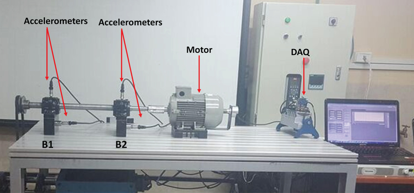
Experimental test bed to extract features from vibration signals for fault severity diagnosis in bearings.

Table 1

Fault conditions in bearing B2

Label	Description	Diameter (mm)	Depth (mm)
P1	Healthy bering	-	-
P2	Inner race	0.5	0.3
P3	Inner race	0.9	0.3
P4	Inner race	1.3	0.3
P5	Outer race	0.5	0.3
P6	Outer race	0.9	0.3
P7	Outer race	1.3	0.3
P8	Rolling element	1	0.5
P9	Rolling element	0.9	0.5
P10	Rolling element	0.8	0.5

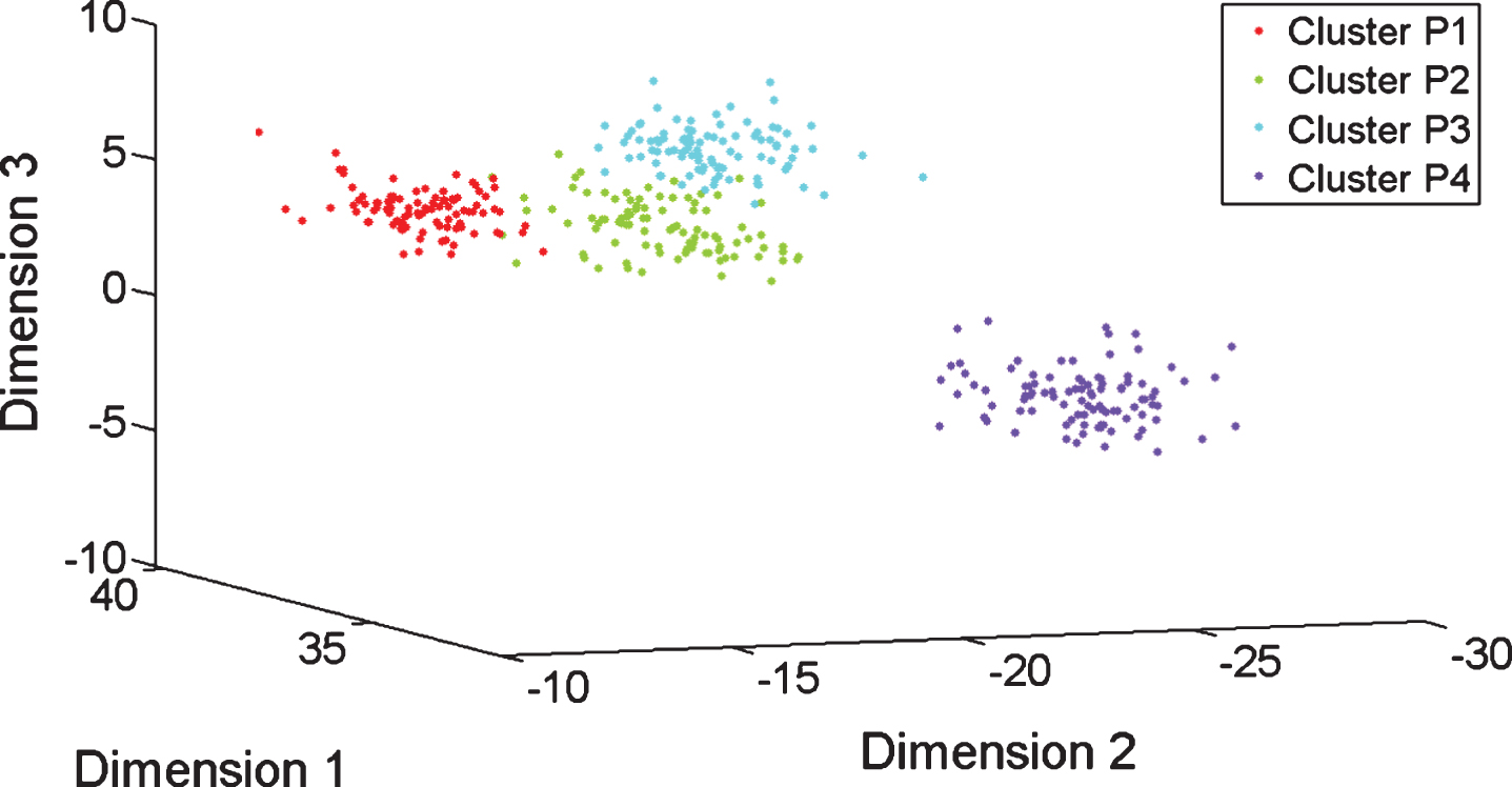
The feature extraction for this case study was performed under the same procedure described in [24], and a set of 663 features for each accelerometer were calculated from 120 samples of vibration signals collected for each fault condition. The resulting dataset has 2652 features and 1200 samples. Our analysis was conducted by considering three different set of fault: (i) P¹ = {P₁, P₂, P₃, P₄}, (ii) P² = {P₁, P₅, P₆, P₇}, (iii) P³ = {P₁, P₈, P₉, P₁₀}. Classical feature selection and reduction techniques were applied to show the performance of the selected features for building adequate clusters. Figures 2 and 3 show the cluster structure obtained from the best three features selected by supervised approaches such as Random Forest (RF) and Linear Discriminant Analysis (LDA), with data from all the four accelerometers in the case (i). Figure 4 shows the performance of the first three features by using the unsupervised technique Principal Components Analysis (PCA). These figures show the associated clusters are overlapped and scattered.

Fig.2

Clusters obtained with the best three dimensional vector of original features by using RF applied over data from four accelerometers in case (i).

Fig.3

Clusters obtained with the best three dimensional vector of artificial features by using LDA applied over data from four accelerometers in case (i).

Fig.4

Clusters obtained with the best three dimensional vector of artificial features by using PCA applied over data from four accelerometers in case (i).

RF selects the best features from the original ones; the selected features are associated with the energy of the wavelet coefficients obtained from the Wavelet Packet Decomposition (WPD) using the wavelet family Daubechies 16. On the contrary, LDA and PCA propose artificial features obtained from the original ones. In this study, the best three artificial features, called Dimension 1, Dimension 2 and Dimension 3, are used as selected features. Next section shows that the proposed approach can select a three dimensional vector of features, from the set of the original features, better than the proposed vector by RF, LDA and PCA, regarding the cluster validity assessment.

5.2 Feature analysis

Our proposed framework presented in Section 4 was used to select the best subset of three features, to build the best clusters oriented to fault severity classification in rolling bearing, for the experimental case described in the previous Section 5. According to some results, classical features for fault diagnosis, as the extracted ones in this work, can be considered close to normal distribution, then ANOVA can be applied [40]. The analysis is performed over the 80% of the available samples. The remaining 20% will be used to test the performance of the selected features in classification. As mentioned previously, the analysis was conducted by considering the three sets of faults P¹, P² and P³. Then, three analysis were performed by using the algorithms in Section 4. In the first step, the set P to apply the Algorithm 1 is composed by the classes in Pⁱ, and all the 2652 features were analysed in the following manner: (i) 1326 features from the accelerometers in the radial position, (ii) 1326 features from the accelerometers in the axial position, and (iii) all the 2652 features from all the four accelerometers.

In order to have statistical significance, the Algorithm 1 is applied for 30 repetitions, over a random selection of the 80% of the samples previously selected for analysis. After applying the algorithm with Th_s = Th_{PW
_s} = 0.05, the result of the selected features is shown in Table 2 regarding the accelerometer placement (ACC), the number of features selected by one-way-ANOVA (NF (p < Th_s)), the number of features selected by the pairwise comparison (NF ( $\hat{p} < {Th}_{{PW}_{s}}$ )), that is, the cardinality of the set F_P, for the corresponding set P = Pⁱ, and the maximum value of the $\hat{p}$ -value (max( $\hat{p}$ )).

Table 2
Results of the Algorithm 1

P ⁱ ACC NF (p < Th_s) NF ( $\hat{p} < {Th}_{{PW}_{s}}$ ) max( $\hat{p}$ )

P ¹ radial 1061 20 0.0291

axial 1054 17 0.0325

all 2115 37 0.0325

P ² radial 1061 40 0.0408

axial 1054 41 0.0486

all 2115 81 0.0486

P ³ radial 1061 39 0.0195

axial 1504 30 0.0497

all 2115 69 0.0497

P ⁱ	ACC	NF (p < Th_s)	NF ( $\hat{p} < {Th}_{{PW}_{s}}$ )	max( $\hat{p}$ )
P ¹	radial	1061	20	0.0291
	axial	1054	17	0.0325
	all	2115	37	0.0325
P ²	radial	1061	40	0.0408
	axial	1054	41	0.0486
	all	2115	81	0.0486
P ³	radial	1061	39	0.0195
	axial	1504	30	0.0497
	all	2115	69	0.0497

In the second step, the Algorithm 2 was applied for each set F_p obtained according to the set of study Pⁱ. Table 3 shows the results regarding each subset Pⁱ, the accelerometers placement, the value of the CDbwF_z for the set f_best, and the individual ranking of the selected features in F_p according to the Equation (9). Table 3 shows that, in fact, the best individual features do not leads to the subset of features having the best value of the CDbwF_z.

Table 3

Results of the Algorithm 2

P ⁱ	ACC	CDbwF _z	R (f₁)	R (f₂)	R (f₃)
P ¹	radial	0.0323	1	4	5
	axial	0.0004	1	2	10
	all	0.0323	1	10	12
P ²	radial	0.0199	20	30	37
	axial	0.0046	18	29	40
	all	0.0412	32	57	58
P ³	radial	0.7488	9	18	31
	axial	1.1156	12	17	21
	all	1.7555	29	31	50

Figures 5, 6 and 7 illustrate the cluster structure obtained with the subset of three features having the maximum value of the CDbwF_z. Axes labels describe the selected features; in most of cases, features related with the energy of the wavelet coefficient from the WPD using the mother wavelet Daubechies 16 were selected. It shows the importance of the time-frequency representation for feature extraction, in the field of fault diagnosis. Particularly, the features in Fig. 5 differs from those ones in Fig. 2 selected for the same case (i) by using RD; the cluster structure in Fig. 5 is better than the cluster structure in Fig. 2. Other selected features were the standard deviation on a certain frequency band, see Fig. 7. In case of P¹, the best value of CDbwF_z is the same with features from the accelerometers in radial position and all the accelerometers, as the same features are selected; then, the information provided by the two axial accelerometers is not useful. In the cases of P² and P³, the best values of CDbwF_z are obtained with features from all the accelerometers. The clusters have adequate overlapping and scattering. Particularly, Fig. 5 shows the selected features produce better cluster structure than that one produced with features selected from RF and PCA, as illustrated in Figs. 2 and 4, respectively. Regarding LDA in Fig. 3, the results of our framework in Fig. 3 makes that the cluster P3 is separated better from P2.

Fig.5

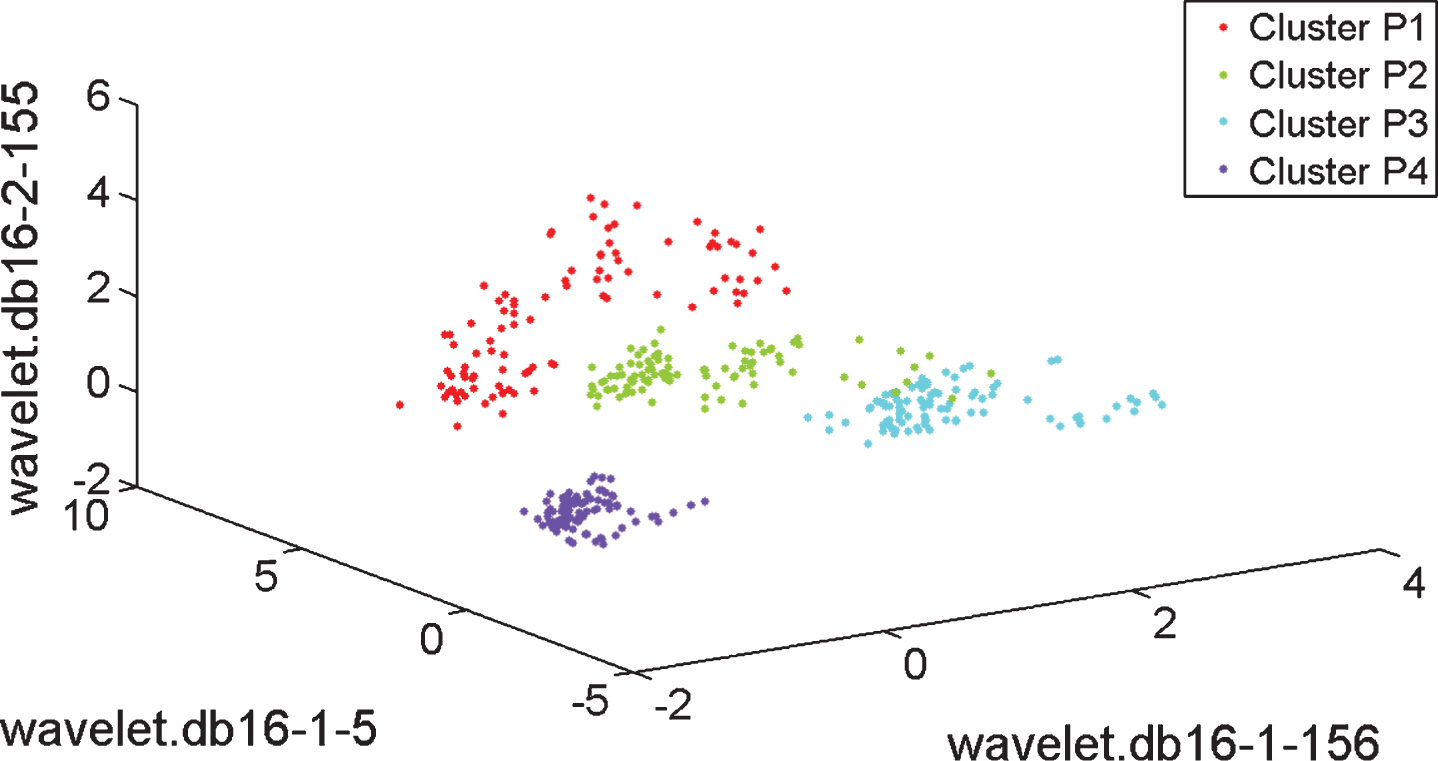
Clusters obtained with the best three dimensional vector of original features by using ANOVA and Clustering Validity Assessment, case (i), four accelerometers.

Fig.6

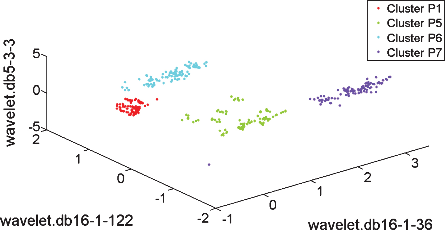
Clusters obtained with the best three dimensional vector of original features by using ANOVA and Clustering Validity Assessment, case (ii), four accelerometers.

Fig.7

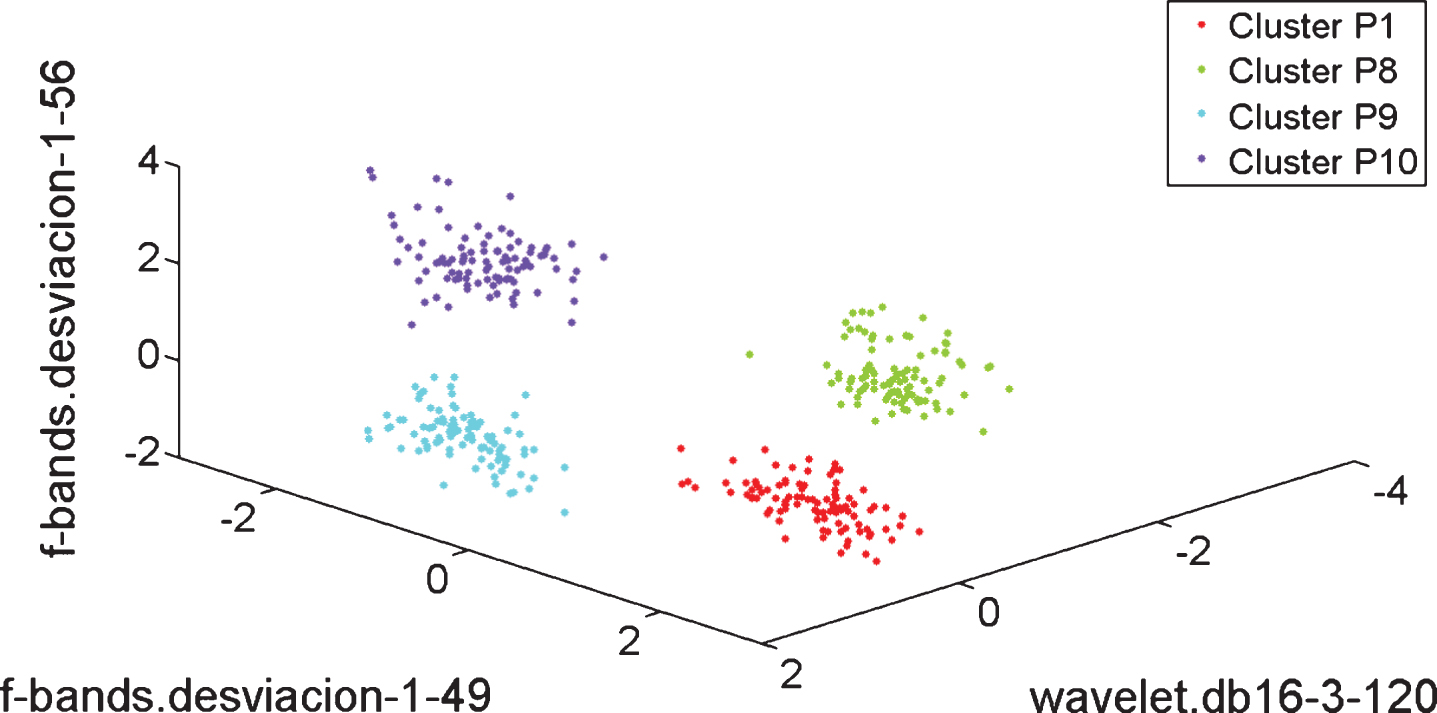
Clusters obtained with the best three dimensional vector of original features by using ANOVA and Clustering Validity Assessment, case (iii), four accelerometers.

5.3 Performance for classification by using feature selection with ANOVA and cluster validity assesment

KNN is a very simple ML algorithm which is widely used to test the performance of feature selection approaches for classification. Clearly, the success of the KNN depends on the cluster structure of the data instances. To test the proposed feature selection, three KNN-based diagnosers have been developed by using each subset of the selected features for the sets P¹, P² and P³. For each case, the performance of classification is measured according to the precision to classify the samples with labels belonging to the corresponding subset Pⁱ, based on the Euclidean Distance (ED) with regard to 20 neighbours.

Additionally, samples s_j with P ∉ Pⁱ are also treated by each classifier in order to measure the ED regarding the closest samples in the class to which the KNN classifier is assigning this sample. Of course, this classification is wrong but the measured distance can be used as useful information to decide if the classification is good or not. Let s_j be a sample with P ∉ Pⁱ that is assigned to a class P_i ∈ Pⁱ, and ${ED}_{\min}^{j}$ is the minimum ED between a sample s_j and a sample s_i into the corresponding labelled cluster. After calculating all the ${ED}_{\min}^{j}$ , three measures are computed according to equations ${ED}_{\min} = \min {{ED}_{\min}^{j}}$ , ${ED}_{\max} = \max {{ED}_{\min}^{j}}$ , and ${ED}_{ave} = Average ({ED}_{\min}^{j})$ .

The previous metrics are defined to have reference values which can be used to define some threshold to suggest if the sample assigned to a class P_i with a specified KNN classifier could be not correct. The design of this threshold is not developed in this work, and the previous measures are only used for analysis purposes. The following classification results are obtained by using the feature selection with signals from all the four accelerometers.

5.3.1 Classification for the set P¹

Table 4 shows the results of classification for the set P¹ with samples having a label P_i ∈ P¹ and P_i ∉ P¹. The precision to classify the faults with labels P₁, P₂, P₃ and P₄ is quite good. The decrement of the precision to classify the class P₂ is due to samples classified as class P₃. In the following rows of the table, the minimum, maximum and average ED of the test samples correctly assigned to the classes, regarding the samples of the class, are stated.

Table 4
Results of KNN based classification, set P¹

P ⁱ Metric P ₁ P ₂ P ₃ P ₄

P_i ∈ P¹ Precision 100% 91.67% 100% 100%

ED _min 0.0788 0.0997 0.0666 0.0220

ED _max 0.5769 0.5510 0.3824 0.3556

ED _ave 0.2677 0.2265 0.1780 0.1118

P_i ∉ P¹ ED _min 0.5996 0.1028 0.3228 0.0525

ED _max 2.0928 1.7232 1.9683 1.6994

ED _ave 1.5281 0.8056 1.0482 0.5358

Samples 18 100 137 707

P ⁱ	Metric	P ₁	P ₂	P ₃	P ₄
P_i ∈ P¹	Precision	100%	91.67%	100%	100%
	ED _min	0.0788	0.0997	0.0666	0.0220
	ED _max	0.5769	0.5510	0.3824	0.3556
	ED _ave	0.2677	0.2265	0.1780	0.1118
P_i ∉ P¹	ED _min	0.5996	0.1028	0.3228	0.0525
	ED _max	2.0928	1.7232	1.9683	1.6994
	ED _ave	1.5281	0.8056	1.0482	0.5358
	Samples	18	100	137	707

In second part of the Table 4 the results by using samples with P_i ∉ P¹ is stated. In this case, 18, 100, 137 and 707 are the number of samples wrongly assigned to class P₁, P₂, P₃ and P₄, respectively. The minimum, maximum and average ED were also calculated. For example, the minimum ED obtained from samples wrongly assigned to P₁ was 0, 5996, this value is up of the maximum ED, and quite up of the average ED, obtained for samples correctly classified. The average ED from of samples wrongly assigned to P₁ was 1, 5281 and this value is quite up of the average ED obtained for the samples correctly assigned to P₁. Then, this information can be used to define some metric or threshold to suggest the sample assigned to a class P₁ with this KNN classifier could be not correct. A similar analysis can be concluded in case of P₃. Then, based on the KNN classifier using the selected features for classes P_i ∈ P¹, the classification of samples in P₃ and P₄ are quite accepted.

In case of the samples with P_i ∉ P¹ wrongly assigned to P₂, the minimum ED was 0, 1028 and this value is up of the minimum ED obtained for the correct samples in P₂, but it is less than the maximum and average values for samples correctly assigned to P₂. It could be not obvious to suggest if the classification is not correct for a sample having a ED into the ranges of the accepted ED for the classification in P₂. However, the average value of the ED obtained for classes wrongly assigned to P₂ are up to the average obtained in the correct assign; then, it is expected a low ratio of samples for which finally, the classification in P₂ is accepted, under some metric. A similar analysis is addressed in case of samples assigned to P₄. Additionally, note that most of the samples with P_i ∉ P¹ were assigned to the class P₄; by comparing the ED_min, ED_max and ED_ave value for this case, it is verified that all these values are lower than the ones in case of P₁, P₂ and P₃.

5.3.2 Classification for the set P²

Table 5 shows the results of classification for the set P² with samples having a label P_i ∈ P² and P_i ∉ P². The precision to classify the faults with labels P₁, P₅, P₆ and P₇ reaches the 100%. In the following rows of the table, the minimum, maximum and average ED of the test samples correctly assigned to the classes, regarding the samples into the cluster, are stated. This values are compared to the obtained ones from samples with P_i ∉ P². In all cases, the metrics are quite up regarding the same metrics for the samples correctly assigned to the class P₂. This result can serve to decide if the new sample belongs truly to a class in P², according to how far the sample is from the most near neighbour in the known classes. As an example of the decision making, most of the samples with the label P_i ∉ P² were assigned to the class P₁, i.e. a false negative can be obtained, however the metrics ED_max and ED_ave are quite different from the metrics in the correct assignment, then the final result can be that this samples is not in the healthy condition P₁.

Table 5
Results of KNN based classification, set P²

P ⁱ Metric P ₁ P ₅ P ₆ P ₇

P_i ∈ P² Precision 100% 100% 100% 100%

ED _min 0.0094 0.0324 0,0371 0.0106

ED _max 0.0878 0.2446 0,1676 0.1924

ED _ave 0.0457 0.0709 0,0901 0.0820

P_i ∉ P² ED _min 0.0273 0.2996 0,6153 2.3394

ED _max 2.2858 3.3259 3.4010 4.5006

ED _ave 1.0861 1.4999 1,8249 3.0847

Samples 656 216 78 10

P ⁱ	Metric	P ₁	P ₅	P ₆	P ₇
P_i ∈ P²	Precision	100%	100%	100%	100%
	ED _min	0.0094	0.0324	0,0371	0.0106
	ED _max	0.0878	0.2446	0,1676	0.1924
	ED _ave	0.0457	0.0709	0,0901	0.0820
P_i ∉ P²	ED _min	0.0273	0.2996	0,6153	2.3394
	ED _max	2.2858	3.3259	3.4010	4.5006
	ED _ave	1.0861	1.4999	1,8249	3.0847
	Samples	656	216	78	10

5.3.3 Classification for the set P³

Table 6 shows the results of classification for the set P³ with samples having a label P_i ∈ P³ and P_i ∉ P³. The precision to classify correctly the faults with labels P₁, P₈, P₉ and P₁₀ reaches the 100%. The minimum, maximum and average ED of the test samples correctly assigned to the classes are calculated, and also these metrics are calculated for the samples that are wrongly assigned to those classes. In this case, the samples with labels P_i ∉ P³ were distributed among the classes in P³, then, with these features, a sample can be assigned equally to any class. However, based on the metrics of the ED, an adequate conclusion regarding the correct diagnosis can be given, taken into account that ED_max and ED_ave are significantly large by comparing with the values in the correct diagnosis.

Table 6
Results of KNN based classification, set P³

P ⁱ Metric P ₁ P ₈ P ₉ P ₁₀

P_i ∈ P³ Precision 100% 100% 100% 100%

ED _min 0.0452 0.0227 0.0514 0.0247

ED _max 0.3396 0.3181 0.5384 0.4761

ED _ave 0.1470 0.1421 0.1621 0.1856

P_i ∉ P³ ED _min 0.0253 0.0572 0.0887 0.0832

ED _max 1.8779 2.1256 2.1304 1.9914

ED _ave 0.5036 0.8137 0.7562 0.8725

Samples 269 267 253 171

P ⁱ	Metric	P ₁	P ₈	P ₉	P ₁₀
P_i ∈ P³	Precision	100%	100%	100%	100%
	ED _min	0.0452	0.0227	0.0514	0.0247
	ED _max	0.3396	0.3181	0.5384	0.4761
	ED _ave	0.1470	0.1421	0.1621	0.1856
P_i ∉ P³	ED _min	0.0253	0.0572	0.0887	0.0832
	ED _max	1.8779	2.1256	2.1304	1.9914
	ED _ave	0.5036	0.8137	0.7562	0.8725
	Samples	269	267	253	171

5.4 Performance for classification by using RF based feature selection

A RF based classifier was developed for each set of faults P¹, P² and P³, with data obtained from all the four accelerometers. The best three features ranked according to the entropy metric are shown in the last column of Table 7. Features extracted from the WPD using the wavelet family Daubechies 16 were always selected, and they differs from those ones selected by our approach, as shown in Figs. 5, 6 and 7. The precision for classification obtained by using the selected features is summarized in Table 7, by using KNN classification. The experimental conditions are the same as proposed in Section 5.3. Then, three different classifiers are considered to classify faults in the sets P¹, P¹ and P³. Regarding the precision reported in Tables 4, 5, and 6, the ability for classification of the proposed three best features by using ANOVA and cluster validity assessment is better than the ability of the three best features selected with RF, in case of P¹ and P²; the same performance is obtained in case of P³. This result shows the improvement of the feature selection as contribution of the approach developed in this work, regarding the classical approach such as RF.

Table 7
Precision in the classification by using features selected with RF

P _i Precision Best three selected features

P ₁ 100% wavelet.db16_3_120

P ₂ 91.67% wavelet.db16_2_122

P ₃ 95.83% wavelet.db16_1_172

P ₄ 95.83%

P ₁ 100% wavelet.db16_3_120

P ₅ 87.50% wavelet.db16_4_178

P ₆ 95.83% wavelet.db16_1_172

P ₇ 95.83%

P ₁ 100% wavelet.db16_2_122

P ₈ 100% wavelet.db16_2_120

P ₉ 100% wavelet.db16_2_129

P ₁₀ 100%

P _i	Precision	Best three selected features
P ₁	100%	wavelet.db16_3_120
P ₂	91.67%	wavelet.db16_2_122
P ₃	95.83%	wavelet.db16_1_172
P ₄	95.83%
P ₁	100%	wavelet.db16_3_120
P ₅	87.50%	wavelet.db16_4_178
P ₆	95.83%	wavelet.db16_1_172
P ₇	95.83%
P ₁	100%	wavelet.db16_2_122
P ₈	100%	wavelet.db16_2_120
P ₉	100%	wavelet.db16_2_129
P ₁₀	100%

6 Conclusion

This paper proposes a two-stage methodological framework that combines ANOVA and cluster analysis to select the best set of features yielding an adequate feature structure for classification tasks in machine learning applications. The framework was applied on the problem of fault severity classification in rolling bearings, and the results were compared to classical feature selection techniques such as RF, LDA, and PCA. The main results of the feature analysis are: (i) The clusters obtained by our framework are better than those ones obtained by the mentioned classical techniques, in terms of the inter-cluster distance and intra-cluster density. This result is useful for the further development of fault classifiers where the cluster structure can determine its performance, (ii) The results also show that the same selection could be obtained from the proposed methodological framework by using accelerometers located in different places. This is an important result to implement fault classifiers in industrial cases where the placement of accelerometers in different locations is not available, (iii) KNN-based classifier was used to test the ability of the cluster structure to produce adequate diagnosis. Several metrics based on the Euclidean Distance of a new sample to the existing clusters were defined as reference values to asses whether a new sample is correctly assigned to the correct class. The results show that a decision-making system could be obtained by combining the metric values from the three classifiers, as the cluster structure for each set of fault is well defined. Future works aim at enhancing the definition of the index CDbwF_z to weight properly the index CDbw associated to a pair of classes, in order to guide the selection of features that improve such specific cluster structure. On the other hand, the metrics defined from the Euclidean Distance could be used in a decision-making system at a third stage, then, several approaches also based on machine learning can be studied.

Acknowledgments

This work was funded by the research division DIUC of the Universidad de Cuenca, through the project “Análisis y definición de estrategias para el desarrollo de sistemas de mantenimiento industrial”, and by the Universidad Politécnica Salesiana under grant No. 002-002-2016-03-03.

References

Cabrera

, Sancho

, Li

, Cerrada

, Sánchez

R.V.

, Pacheco

, Valente de Oliveira

, Automaticfeature extraction of time-series applied to fault severity assessment of helical gearbox in stationary andnon-stationary speed operation, Applied Soft Computing58 (2017), 53–64.

Cerrada

, Sánchez

R.V.

, Cabrera

, Zurita

, Li

, Multi-stage feature selection by using geneticalgorithms for fault diagnosis in gearboxes based on vibration signal, Sensors15 (9) (2015), 23903–23926.

Cerrada

, Sánchez

R.V.

, Li

, Pacheco

, Cabrera

, Valente de Oliveira

and Vásquez

R.E.

, Areview on data-driven fault severity assessment in rolling bearings, Mechanical Systems and SignalProcessing99 (2018), 169–196.

Cerrada

, Zurita

, Cabrera

, Sánchez

R.V.

, Artés

, Li

, Fault diagnosis in spur gears basedon genetic algorithm and random forest, Mechanical Systems and Signal Processing70-71 (2016), 87–103.

Chandrashekar

, Sahin

, A survey on feature selection methods, Computers & Electrical Engineering40 (1) (2014), 16–28.

Chen

C.H.

, Feature selection based on compactness and separability: Comparison with filter-based methods, Computational Intelligence30 (3) (2014), 636–656.

Chen

C.H.

, Feature selection for clustering using instancebased learning by exploring the nearest and farthestneighbors, Information Sciences318 (2015), 14–27.

Cox

, Anusonti-Inthra

, Turbine engine rotor blade fault diagnostics through casing pressure and vibrationsensors, Journal of Physics: Conference Series548 (1) (2014), 012066.

Duque-Perez

, Garcia-Escudero

L.A.

, Morinigo-Sotelo

, Gardel

P.E.

, Perez-Alonso

, Analysis of faultsignatures for the diagnosis of induction motors fed by voltage source inverters using ANOVA and additivemodels, Electric Power Systems Research121 (2015), 1–13.

10.

Ftoutou

, Chouchane

, Besbès

, Internal combustion engine valve clearance fault classification usingmultivariate analysis of variance and discriminant analysis, Transactions of the Institute of Measurementand Control34 (5) (2012), 566–577.

11.

Gheyas

I.A.

, Smith

L.S.

, Feature subset selection in large dimensionality domains, Pattern Recognition43 (1) (2010), 5–13.

12.

Hai

, Tsui

K.L.

, Zuo

M.J.

, Gear crack level classification based on multinomial logit model and cumulativelink model. In Prognostics and System Health Management (PHM), 2012 IEEE Conference on, IEEE, 2012, pp. 1–6.

13.

Halkidi

, Vazirgiannis

, Clustering validity assessment using multi representatives, In Proceedingsof the Hellenic Conference on Artificial Intelligence, SETN, 2002, pp. 237–249.

14.

Johnson

K.J.

, Synovec

R.E.

, Pattern recognition of jet fuels: Comprehensive GC x GC with ANOVA-based featureselection and principal component analysis, Chemometrics and Intelligent Laboratory Systems60 (1-2) (2002), 225–237.

15.

Lei

, Intelligent Fault Diagnosis and Remaining Useful Life Prediction of Rotating Machinery. Butterworth-Heinemann; Oct 2017.

16.

, Sanchez

R.V.

, Zurita

, Cerrada

, Cabrera

, Fault diagnosis for rotating machinery using vibrationmeasurement deep statistical feature learning, Sensors16 (6) (2016).

17.

, Sanchez

R.V.

, Zurita

, Cerrada

, Cabrera

, Vasquez

R.E.

, Multimodal deep support vectorclassification with homologous features and its application to gearbox fault diagnosis, Neurocomputing168 (2015), 119–127.

18.

, Sanchez

R.V.

, Zurita

, Cerrada

, Cabrera

, Vasquez

R.E.

, Gearbox fault diagnosis based on deeprandom forest fusion of acoustic and vibratory signals, Mechanical Systems and Signal Processing76-77 (2016), 283–293.

19.

, Valente de Oliveira

, Cerrada

, Pacheco

, Cabrera

, Sánchez

R.V.

and Zurita

, Observer-biased bearing condition monitoring: From fault detection to multi-fault classification, Engineering Applications of Artificial Intelligence, in press 2018.

20.

Liu

, Wu

, Zhang

, A new supervised feature selection method for pattern classification, Computational Intelligence30 (2) (2014), 342–361.

21.

Maldonado

, Carrizosa

, Weber

, Kernel penalized k-means: A feature selection method based on kernelk-means, Information Sciences322 (2015), 150–160.

22.

Niknam

S.A.

, Songmene

, Au

Y.H.J.

, The use of acoustic emission information to distinguish between dry andlubricated rolling element bearings in low-speed rotating machines, The International Journal of AdvancedManufacturing Technology69(9) (2013), 2679–2689.

23.

Ott

R.L.

, Longnecker

M.T.

, An introduction to statistical methods and data analysis. Cengage Learning, Boston, Massachusetts; 2015.

24.

Pacheco

, Cerrada

, Sánchez

R.V.

, Cabrera

, Li

, Valente de Oliveira

, Attribute clusteringusing rough set theory for feature selection in fault severity classification of rotating machinery, Expert Systems with Applications71 (2017), 69–86.

25.

Pacheco

, Valente de Oliveira

, Sánchez

R.V.

, Cerrada

, Cabrera

, Li

, Zurita

and Artés

, A statistical comparison of neuroclassifiers and feature selection methods for gearbox fault diagnosis underrealistic conditions, Neurocomputing194 (2016), 192–206.

26.

Peng

, Long

, Ding

, Feature selection based on mutual information criteria of max-dependency,max-relevance, and min-redundancy, IEEE Transactions on pattern analysis and machine intelligence27 (8) (2005), 1226–1238.

27.

Pierce

K.M.

, Hope

J.L.

, Johnson

K.J.

, Wright

B.W.

, Synovec

R.E.

, Classification of gasoline data obtained bygas chromatography using a piecewise alignment algorithm combined with feature selection and principal componentanalysis, Journal of Chromatography A1096 (1-2) (2005), 101–110.

28.

Shi

, Li

, Han

, Hu

, Cluster structure preserving unsupervised feature selection for multi-viewtasks, Neurocomputing175 (Part A) (2015), 686–697.

29.

Sim

, Ramli

, Saifizul

, Abdullah

, Empirical investigation of acoustic emission signals for valvefailure identification by using statistical method, Measurement58 (2014), 165–174.

30.

Verma

, Sarangi

, Kolekar

, Stator winding fault prediction of induction motors using multiscale entropyand grey fuzzy optimization methods, Computers & Electrical Engineering40 (7) (2014), 2246–2258.

31.

Watson

N.E.

, VanWingerden

M.M.

, Pierce

K.M.

, Wright

B.W.

, Synovec

R.E.

, Classification ofhigh-speed gas chromatography-mass spectrometry data by principal component analysiscoupled with piecewise alignment and feature selection, Journal of Chromatography A1129 (1) (2006), 111–118.

32.

Wei

, Wang

, He

, Bao

, A novel intelligent method forbearing fault diagnosis based on affinity propagation clustering and adaptive feature selection, Knowledge-Based Systems116 (Supplement C) (2017), 1–12.

33.

, Chow

T.W.

, Clustering of the self-organizing map using a clustering validity index based oninter-cluster and intra-cluster density, Pattern Recognition37 (2) (2004), 175–188.

34.

, Wang

, Bu

, Chen

, Group sparse feature selection on local learning based clustering, Neurocomputing171 (2016), 1118–1130.

35.

Yoon

, He

, Van Hecke

, On the use of a single piezoelectric strain sensor for wind turbine planetarygearbox fault diagnosis, IEEE Transactions on Industrial Electronics62 (10) (2015), 6585–6593.

36.

Yuwono

, Guo

, Wall

, Li

, West

, Platt

, Su

S.W.

, Unsupervised feature selection using swarmintelligence and consensus clustering for automatic fault detection and diagnosis in heating ventilation and airconditioning systems, Applied Soft Computing34 (2015), 402–425.

37.

Yuzukirmizi

, Arslan

, Fault diagnosis of shaft-ball bearing system using one-way analysis of variance, Mathematical and Computational Applications19 (1) (2014), 37–49.

38.

Zanoli

S.M.

, Astolfi

, Application of a fault detection and isolation system on a rotary machine, International Journal of Rotating Machinery2013 (2013).

39.

Zhang

, Ma

, He

, Fault diagnosis model based on fuzzy support vector machine combined withweighted fuzzy clustering, Transactions of Tianjin University19 (3) (2013), 174–181.

40.

Zhang

, Hu

, Cheng

, A condition indicator performance assessment method based on signaldetection theory, In Prognostics and System Health Management Conference (PHM-Chengdu), 2016, IEEE, (2016), pp. 1–5.

Feature engineering based on ANOVA,cluster validity assessment and KNN for fault diagnosis in bearings

Abstract

Keywords

1 Introduction

2 Related works

3 Background

3.1 Analysis of Variance (ANOVA) and Tukey’s test

5.1 Experimental text bed

Table 2 Results of the Algorithm 1 P i ACC NF (p < Th s ) NF ( p ˆ < Th PW s ) max( p ˆ ) P 1 radial 1061 20 0.0291 axial 1054 17 0.0325 all 2115 37 0.0325 P 2 radial 1061 40 0.0408 axial 1054 41 0.0486 all 2115 81 0.0486 P 3 radial 1061 39 0.0195 axial 1504 30 0.0497 all 2115 69 0.0497

5.3.1 Classification for the set P1

Acknowledgments

References

5.3.1 Classification for the set P¹