Fault diagnosis based on orthogonal semi-supervised LLTSA for feature extraction and Transductive SVM for fault identification

Abstract

To overcome the low diagnosis accuracy caused by the scarcity of labeled training samples, a fault diagnosis method was proposed using orthogonal Semi-supervised linear local tangent space alignment (OSSLLTSA) for feature extraction and transductive support vector machine (TSVM) for fault identification. Through extracting the statistical features were extracted from the sub-bands of vibration signals decomposed by wavelet packet decomposition (WPD), the high-dimensional feature set could be obtained. Following that, the improved kernel space distance evaluation method was applied to remove non-sensitive fault features. Then, a semi-supervised manifold learning method (OSSLLTSA) was proposed to reduce the dimensionality of the fault feature set, and thus to extract fused fault features with high clustering performance. OSSLLTSA overcomes the over-learning of supervised manifold learning and projection aimlessness of unsupervised manifold learning. Finally, the low-dimensional feature set after dimension reduction was inputted into TSVM for fault diagnosis. TSVM was able to completely utilize the fault information contained in unlabelled samples to modify the model, and the trained fault diagnosis model has better generalization ability. The effectiveness of the proposed method was verified based on the case of gearbox fault. Experimental results showed that the proposed method is able to achieve very high fault diagnosis accuracy even when labeled samples were insufficient.

Keywords

Fault diagnosis semi-supervised manifold learning gearbox transductive support vector machine

1 Introduction

Rotating machinery has become increasingly more important in modern industry, such as wind turbine, steam turbine, etc. However, many factors can cause faults during operation of rotating machines, including poor lubrication, fatigue damage, wear and harsh running environment, etc. It has been reported that gearbox faults account for 11% of total wind turbine faults, and bearing faults account for 44% of total faults in large induction motors [1, 2]. Fortunately, accurate identification of running states can well monitor the condition of machinery and diagnosis the occurring fault, by which the repair time and cost is reduced and economic loss can be avoided in large degree. Currently, machinery condition monitoring and fault diagnosis has developed as an important research issue in mechanical engineering.

The vibration signal generated during operation is the key reference for analyzing rotating machines and their running states. However, the vibration signal has very complicated frequency components and is always non-stationary and nonlinear state. So effectively extracting fault features is essential for machinery fault diagnosis. Many research works have pointed out that energy or information distribution in each frequency band of vibration signals varies with the change of running states, for example D. Wang and C.Q. Shen et al. [3, 4] applied statistical parameters of wavelet packet paving to fault diagnosis of bearings and gears, Y.N. Pan [5] applied wavelet packet node energies to track bearing health. Therefore, wavelet packet decomposition (WPD) was adopted to decompose vibration signals into several sub-bands [6], and then statistical features are extracted from each frequency sub-band to obtain a high-dimensional feature set. The fault features extracted from each sub-bands are more sensitive than those being directly extracted from original vibration signals, and the former is able to more effectively characterize machinery running states. However, the high-dimensional fault feature set contains a large amount of redundant information and noise, therefore it is still a challenging problem to extract the most useful fault information from the high-dimensional fault feature set. Dimensionality reduction can largely compress the dimension of fault feature set and maintain the essential information of original feature sets. Commonly used dimensionality reduction methods include principle component analysis (PCA) [7], multidimensional scaling (MDS) [8], independent component analysis (ICA) [9], etc. These methods are easy to implement with small amount of calculation and stable performance. However, these linear dimensionality reduction methods are inadequate in handling fault data sets with non-linearity and non-Gaussian structures. Manifold learning, represented by local linear embedding (LLE) [10], Isomap [11], local tangent space alignment (LTSA) [12], etc., is a kind of non-linear dimensionality reduction method, which can effectively extract the non-linear structural information contained in datasets. To meet the demand of pattern recognition and fault diagnosis, a number of improved manifold learning methods have been proposed, including the linear improvements of manifold learning, such as neighborhood preserving embedding (NPE) [13], locality preserving projection (LPP) [14], linear local tangent space alignment (LLTSA) [15], etc. These improved methods give out the explicit mapping from input space to low-dimensional feature space, and solve the problem of “out of sample”, therefore, they are more efficient and practical. However, these methods did not take the supervisory role of class label information into consideration. As a pattern recognition problem, one of the main purposes of dimensionality reduction in fault diagnosis is to enlarge diversity of the fault samples. To the end, some supervised variants have been proposed, such as supervised LPP [16], supervised LLTSA (SLLTSA) [17], etc. These methods have already been applied in machinery fault diagnosis [18, 19]. However, in machinery fault diagnosis, labeling fault samples is usually costly and time-consuming, which means that one may always face situation of scarcity of labeled training samples when diagnosing machinery faults. Worse still, supervised methods will be prone to over-learning if labeled training samples are not enough. On the other hand, unlabelled samples are easy to access, so over-learning problem can be relieved or even avoided if information contained in unlabelled samples is used to improve dimensionality reduction process. To deal with this problem, a semi-supervised manifold learning method, orthogonal semi-supervised LLTSA (OSSLLTSA), was proposed based on LLTSA. OSSLLTSA is able to simultaneously extract the structural information contained in labeled and unlabelled samples, overcoming the over-learning of supervised manifold learning and projection aimlessness of unsupervised manifold learning. OSSLTSA also adopts orthogonal iteration method to solve the orthogonal mapping matrix from high-dimensional observation space to low-dimensional feature space, which make it possible to rapidly calculate the optimal low-dimensional coordinates of high dimensional fault samples.

The fault diagnosis of rotating machinery is essentially a pattern recognition problem. Therefore, after feature extraction, pattern recognition algorithms are needed for realizing fault diagnosis or classification after feature extraction. Commonly used pattern recognition algorithms include k-nearest-neighbors classifier (KNNC) [20], artificial neural network (ANN) [21], support vector machine (SVM) [22], etc. As a pattern recognition method based on data statistics, KNNC requires a large numbers of labeled samples for model training, while ANN algorithm easily suffers from over-learning and local optima problems due to using empirical risk minimization criterion. SVM is a kind of pattern recognition algorithm based on structural risk minimization, which can effectively overcome over-learning and local optima problems. SVM has been widely used in machinery fault diagnosis and condition monitoring [23, 24]. However, in the case of lacking labeled samples, the classification hyperplane obtained by SVM seriously deviates from the optimal classification hyperplane, causing unsatisfactory fault recognition accuracy. Transductive SVM (TSVM) [25] is the semi-supervised improvement of SVM, and which can realize model training using the mixture of labeled and unlabelled samples, and modify the model using the fault information in unlabelled samples. The trained fault diagnosis model has better generalization ability. Based on OSSLLTSA and TSVM, a new fault diagnosis method was proposed in this study. Firstly, high dimensional fault features were extracted from vibration signals. Then, OSSLLTSA algorithm was adopted to reduce the dimension of the high dimensional fault feature set and extract out fused fault features with low dimension and high clustering performance. Finally, the fused fault features were inputted into TSVM for fault pattern recognition.

The rest of this paper is organized as follows. In Section 2, the feature extraction by semi-supervised manifold learning is described, and algorithm of Transductive support vector machine is discussed in section 3. Then, a new method for machinery fault diagnosis is presented in Section 4. Experiment set up and signal acquisition is described in Section 5. Following that, fault diagnosis test is performed in Section 6 to verify the proposed method. Finally, some conclusions are drawn in Section 7.

2 Feature extraction by semi-supervised LLTSA

2.1 High-dimensional fault feature set

2.1.1 Original fault feature set extraction

The vibration signals generated during operation of rotating machinery contain rich running states information. The statistic features in time and frequency domains can directly reflect the change of vibration signals and thus characterize different types of faults [26]. When the machinery running states changes, the energy distribution of vibration signals in each sub-band also accordingly changes [27]. The distribution and the information amount contained in each sub-band also vary with the change of running states [28]. Moreover, autoregressive (AR) model parameters are also very sensitive to running states variation [29]. However, the frequency components of vibration signal with non-stationary and non-linear characters, making it difficult to extract effective fault features from original vibration signals. Therefore, WPD was firstly adopted to decompose vibration signals into several sub-bands. Then, the vibration signals in each sub-bands were processed to extract 8 statistical features in both time and frequency domain, including mean value, peak value, root mean square, standard deviation, waveform factor, kurtosis, mean frequency, standard deviation of frequency. AR model parameters, instantaneous amplitude, Shannon entropy, and wavelet packet energy feature are used to form the original high dimensional fault feature set. The definition and calculation methods of relevant features are described in [30].

2.1.2 Fault feature selection

The original high dimensional feature set extracted from vibration signals is inevitably mixed with insensitive features or even interference noise features, which will not only increases computational burden, but also affects the accuracy of fault recognition. Therefore, feature selection for the original feature set is needed to remove the insensitive and interference noise features. Distance evaluation method is a simple and applicable method for sensitive feature selection. However, the performance of this method is largely affected by outliers. To deal with this problem, a kernel space distance evaluation method which uses kernel space distance as discrimination criterion was proposed [31, 32]. Given that there is a feature set containing K classes of states, {f_i,k,j, i = 1, …, I_k, k = 1, …, K, j = 1, …, J}, where I_k is the number of samples in the k-th class, K is the number of states, and J is the number of features. The implementation of the kernel space distance evaluation method is shown in Table 1. It is clear from the implementation process that the larger the ${\bar{ω}}_{j}$ of a feature is, the more sensitive the feature will be.

Table 1
Implementation of kernel space distance evaluation method

(1) Calculate the average distance between samples of the same class.

$d_{k, j} = 1 / - I_{k} \sum_{i = 1}^{I_{k}} D (f_{i, k, j}, 1 / - I_{k} \sum_{i - 1}^{I_{k}} {\bar{f}}_{i, k, j}), i = 1, 2 \dots I_{k}, k = 1, 2, \dots, K, j = 1, 2, \dots, J$

where $D (x, y) = \sqrt{2 - 2 K_{σ} (x, y)}$ is the distance between samples in kernel space and K_σ is kernel function.

Then calculate the within-class scatter of the sample set.

$S_{j}^{W} = 1 / - k \sum_{k = 1}^{K} d_{k, j}$

(2) Calculate the distance between the k-th class of states and the k′-th class of states. (k′ = 1, 2, …, K)

$d_{j}^{k, k^{'}} = 1 / - (I_{k} I_{k^{'}}) \sum_{i = 1}^{I_{k}} \sum_{i^{'} = 1}^{I_{k^{'}}} D (f_{i, k, j}, f_{i^{'}, k^{'}, j})$

Then calculate the average inter-class distance of sample set.

$S_{j}^{b} = \frac{1}{K (K - 1)} \sum_{k = 1}^{K} \sum_{k^{'} = 1}^{K} d_{j}^{{kk}^{'}}$

(3) Fianally calculate the sensitivity degree

$ω_{j} = S_{j}^{B} / - S_{j}^{W}$

For further processing normalization is made for ω_j, i.e., ${\bar{ω}}_{j} = ω_{j} / - max (ω_{j})$ .

2.2 Algorithm of orthogonal semi-supervised LLTSA

By feature selection, the interference information in feature set can be preliminarily removed. However, the non-linear coupling relation between features also exists, causing large amounts of redundant information existing in the feature set. This redundant information can directly affect the accuracy of further fault diagnosis.

Therefore, we need to perform non-linear dimensionality reduction for the high dimensional feature set to extract fused fault feature vector with low dimension, good clustering performance and high sensitivity degree. For this, OSSLLTSA was proposed based on LLTSA algorithm, in order to extract sensitive fault features in the high dimensional feature set.

2.2.1 Brief review of LLTSA

The basic idea of LLTSA is that the local geometric structure of a data set can be represented by low dimensional local tangent space. Performing global alignment for the obtained local tangent space can realize the attribute reduction of high dimensional sample set. Given the high dimensional data set X ={ x_i ∈ R^D, i = 1, …, N }, the implementation of LLTSA mainly includes the following steps.

Constructing local neighborhoods. For each data sample x_i, (i = 1, …, N), k neighboring points are selected from X according to Euclidean distance, forming the local neighborhood of this sample, X_i = [x_i1, …, x_ik].

Obtaining the neighborhood tangent space. Find a set of orthogonal bases, Q_i, from the local neighborhood X_i of data sample x_i, and project X_i to Q_i in order to extract the main geometric structural information of the neighborhood, i.e., $arg min_{Q_{i}, Ω_{i}} {∥ X_{i} H_{k} - Q_{i} Ω_{i} ∥}^{2}$ (1) Wherein H_k = I - ee^T/ - k is the centralized matrix, and the local low dimensional coordinates of X_i is $Θ_{i} = Q_{i}^{T} X_{i} H_{k}$ .

Global alignment of local tangent space. The global alignment of local tangent space is indeed the reconstruction process for the intrinsic structure of data set, and it can be converted into the approximate solution process of a minimization problem. $arg min_{Y} \sum_{i = 1}^{N} E_{i} = arg min_{Y} \sum_{i = 1}^{N} {∥ Y_{i} H_{k} - L_{i} Θ_{i} ∥}^{2}$ (2)

where Y_i is the global low dimension coordinates of X_i, and L_i is local transform matrix. When

L_{i} = Y_{i} H_{k} Θ_{i}^{+}

, the reconstruction error is the minimum.

Θ_{i}^{+}

is the Moore-Penrose generalized inverse of Θ_i. Finally, the solution of the minimization in Equation (2) is converted into the solution of generalized eigenvalue as follows.

{XH}_{N} {BH}_{N} X^{T} α = λ {XH}_{N} X^{T} α

(3) where

B = SVV^TS^T is global alignment matrix;

S = [S₁, S₂, …, S_N];

S_i is a selection vector;

V = diag (V₁, V₂, …, V_N);

$V_{i} = H_{k} (I - Θ_{i}^{+} Θ_{i})$ .

The generalized eigenvectors corresponding to the first d, (d << D) minimum non-zero generalized eigenvalue in Equation (3) form a matrix A = [α₁, α₂, …, α_d], which is the mapping matrix from high dimensional observation space to low dimensional feature space. The low dimensional global coordinates of data sample set X is Y = A^TXH_k.

2.2.2 Algorithm of orthogonal semi-supervised LLTSA

In the case of lacking labeled samples are insufficient, supervised manifold learning will suffer from over-learning problem in feature extraction, while unsupervised manifold learning has projection aimlessness in feature extraction. An orthogonal semi-supervised linear local tangent space alignment (OSSLLTSA) algorithm was proposed to integrate sample class information into dimensionality reduction process, so as to guide feature extraction and improve the discriminability of high dimensional features. Given a sample set X {x₁, x₂, …, x_L, x_L+1, x_L+2, …, X_N} containing N training samples, where X^L ={ x₁, …, x_L } is labeled training samples, and X^U ={ x₁, …, x_N } is unlabelled training samples, then the implementation steps of OSSLLTSA algorithm are as follows.

Constructing the local neighborhood of sample points

When the local neighborhood X_i of sample point x_i is constructed, for labeled training samples x_i, i = 1, …, L, a supervised method is used to select neighboring points. The distance between samples is redefined in constructing neighborhood [26]: $\bar{D_{ij}} = {\begin{matrix} \sqrt{e^{D_{ij}^{2} / - λ} - σ}, l_{i} \neq l_{j} \\ \sqrt{1 - e^{- D_{ij}^{2} / - λ}}, l_{i} = l_{j} \end{matrix}$ (4) where

l_i, i = 1, …, L are the class labels of x_i;

D_ij, i, j = 1, …, L is the distance between samples x_i and x_j;

λ is the distance penalty parameter and usually set to the average distance between samples;

σ ∈ [0, 1] is an adjustment coefficient;

for unlabelled training sample x_i, i = L + 1, …, N, Euclidean distance is adopted for selection in training sample set X.

Constructing objective function

According to the implementation process of LLTSA algorithm, it can be known that the essence of dimension reduction is to realize the extraction of local tangent space using local PCA algorithm. It was proved in [34] that using MDS for extracting local tangent space is equivalent to local PCA. Moreover, the distance information can be sufficiently utilized when MDS is used for extracting local tangent space. Given the squared distance matrix of local neighborhood, $Ω_{i} = {[d_{lj}]}_{l, j = 1}^{k}$ , where d_lj is the distance between samples x_il and x_ij which are nearest to sample d_lj. The distance d_lj can be either the Euclidean distance or the redefined distance between samples. The detailed calculation process, by using MDS to extract the local low dimensional coordinates of X_i, is as follows. $H_{k} Ω_{i} H_{k} = U_{i} diag (λ_{1}, \dots, λ_{k}) U_{i}^{T}$ (5) $where λ_{1} \geq λ_{2} \geq, \dots, \geq λ_{k}$

It is clear in the above equation that the local low dimensional coordinates of X_i is $Θ_{i} = diag (\sqrt{λ_{1}}, \dots, \sqrt{λ_{d}}) V_{i}^{T}$ , where V_i is composed of the first d column vectors of U_i.

The local neighborhood X_i of sample x_i is an approximately linear space, and therefore, X_i can be used to reconstruct x_i.

$\begin{matrix} ω_{i} = arg min_{W_{i}} (\sum_{j = 1}^{k} {∥ x_{i} - ω_{ij} x_{j}^{i} ∥}^{2}) \\ subject to \sum_{j = 1}^{k} ω_{ij} = 1 \end{matrix}$ (6)

Clearly, reconstruction coefficient ω_ij reflects the importance or contribution of x_ij in reconstructing x_i. The larger the reconstruction coefficient ω_ij is, the higher the probability that sample points x_ij and x_i are from the same class is. Therefore, in constructing squared distance matrix, the reconstruction coefficient can be used to weight the distance between samples. To avoid too big weighted distance between samples caused by small or negative ω_ij, ω_ij is preprocessed as Equation (7). ${\bar{ω}}_{ij} = η | ω_{ij} | / - \sum_{j = 1}^{k} | ω_{ij} |, if {\bar{ω}}_{ij} < φ {\bar{ω}}_{ij} = φ$ (7)

It is clear from Equation (7) that the value range of ${\bar{ω}}_{ij}$ is [φ η), where φ < 1 < η. Finally, the weighted distance between samples is $d_{ij} = D_{ij} / - {\bar{ω}}_{ij}$ .

For samples x_i, i = L + 1, …, N, since the neighborhood contains at least one unlabelled sample, in constructing the weighted distance matrix of local neighborhood, only the distances between x_i, i = 1, …, L and the neighboring samples x_ij, j = 1, …, k are weighted. The nearest neighboring samples x_ij, j = 1, …, k of sample x_i, i = 1, …, L are completely labeled samples. Therefore, in constructing the weighted distance matrix of local neighborhood, all the inter-class distances of local neighborhood X_i are weighted, and the two limit values of ${\bar{ω}}_{ij}$ , η and φ are weighted. $d_{ln} = {\begin{matrix} D_{ln} / - η if l_{l} \neq l_{n} \\ D_{ln} / - φ if l_{l} = l_{n} \end{matrix}, l, n = 1, \dots, k$ (8)

From the above analysis, it can be known that after weighting the inter-class distance within local neighborhood, the inter-class distance within the same class is compressed while the distance between samples of different classes is stretched. Therefore, MDS was used to extract the local structural information of sample neighborhood, so as to effectively separate samples in different classes in local neighborhoods. The average distance matrix of local neighborhood constructed by using weighted distance was adopted, and MDS algorithm was used to calculate the local low dimensional coordinates $Θ_{i} = diag (\sqrt{λ_{1}}, \dots, \sqrt{λ_{d}}) V_{i}^{T}$ of neighborhood X_i. The obje -ctive function of dimensionality reduction is obtained by substituting Θ_i, i = 1, …, N into Equations (2) and (3).

Solving orthogonal mapping matrix

The advantage of using orthogonal mapping lies in that the low dimensional fault sample set after dimensionality reduction also maintains the geometric structural information contained in high dimensional fault sample set. Compared with non-orthogonal mapping, orthogonal mapping has better discriminability. Let the mapping matrix be M, and then after dimensionality reduction of any two samples ξ_i, ξ_j by M, the distance calculation in low dimensional sub-space is as follows.

$\begin{matrix} dist (M^{T} ξ_{i}, M^{T} ξ_{j}) = ∥ M^{T} ξ_{i} - M^{T} ξ_{j} ∥ \\ = ∥ M^{T} (ξ_{i} - ξ_{j}) ∥ \\ = \sqrt{{(ξ_{i} - ξ_{j})}^{T} {MM}^{T} (ξ_{i} - ξ_{j})} \end{matrix}$ (9)

If the mapping matrix M is an orthogonal matrix, MM^T = I (where I is an identical matrix). It is clear that the orthogonal projection of ξ_i, ξ_j does not change the distance between samples, which maintains the geometric structural information contained in the original sample set. Therefore, orthogonal iteration method was adopted in this study to calculate the orthogonal mapping matrix from high dimensional observation space to low dimensional feature space. The detailed derivation and calculation process of orthogonal iteration algorithm are referred to literature [35]. Let Ψ ={ ψ₁, …, ψ_d } be the orthogonal base vector of the orthogonal mapping matrix to be solved, and define two matrices, namely ψ^(m-1) = [ψ₁, …, ψ_m-1] , m = 2, …, d and Φ^(m-1) = (Ψ^m-1) ^T (XH_NX^T) Ψ^m-1. The calculation steps of orthogonal iteration are as follows.

Calculate the eigenvector corresponding to the minimum eigenvalue of Equation (3), and define this eigenvector as ψ₁;

Calculate the following orthogonal optimization objective function;

$\begin{matrix} T^{(m)} \\ = {I - {({XH}_{N} X^{T})}^{- 1} Ψ^{(m - 1)} {[Φ^{(m - 1)}]}^{- 1} \\ {[Ψ^{(m - 1)}]}^{T}} \cdot {({XH}_{N} X^{T})}^{- 1} ({XH}_{N} {BH}_{N} X^{T}) \end{matrix}$ (10) where the eigenvector corresponding to the minimum eigenvalue in Equation (10) is ψ_m.

Repeat the above process until all orthogonal base vectors Ψ ={ ψ₁, …, ψ_d } of the orthogonal mapping matrix are solved. Then the mapping process from high dimensional observation space to low dimensional feature space is Y = Ψ^TXH_N. To avoid singular matrices generated in dimensionality reduction, PCA transform can be performed for the original data set, and the finally obtained mapping matrix is Ψ_PCAΨ.

3 Algorithm of transductive support vector machine (TSVM)

SVM is a kind of pattern recognition algorithm which realizes actual risk minimization based on structural risk minimization. SVM can realize the class recognition of test samples by constructing a classification hyperplane composed of a few support vectors, moreover, it has advantage in dealing with small sample sets and non-linear pattern recognition. However, when there are too few labeled samples, the classification hyperplane trained by SVM deviates from the optimal hyperplane, reducing the fault diagnosis accuracy. TSVM algorithm is a semi-supervised improvement of SVM, which uses both labeled and unlabelled samples for model training. The sample distribution information contained in unlabeled samples is used to modify the classification hyperplane, so that the finally obtained final classification hyperplane approaches the optimal hyperplane.

Assume there are a labeled training sample set S^l = { (x_i, y_i) } , x_i ∈ R^d, y_i ∈ { - 1, + 1 } , i = 1, …, L, and an unlabeled training sample set $S^{u} = {x_{i}^{*}}, x_{i}^{*} \in R^{d}, i = 1, \dots, N$ . TSVM simultaneously uses S^l and S^u for model training, i.e., the training sample set of TSVM is S^l ∪ S^u. TSVM algorithm uses transductive training model to obtain classification decision mechanism, and predict the label information, $y_{i}^{*}, i = 1, \dots, N$ , of unlabelled training samples. The training objective of TSVM is maximizing the geometric interval of the optimal classification hyperplane f (x) = wx + b = 0, i.e., maximizing 2/ -∥ w ∥. An equivalent objective function is adopted for TSVM by solving the optimal classification hyperplane.

$\begin{matrix} min_{w} Φ (w) = {∥ w ∥}^{2} \\ s . t . \forall_{i = 1}^{l} y_{i} ({wx}_{i} + b) \geq 1 \\ \forall_{i = 1}^{N} y_{i}^{*} ({wx}_{i} + b) \geq 1 \end{matrix}$ (11) where

w is the normal vector of the optimal classification hyperplane;

b is the offset;

$y_{i}^{*}, i = 1, \dots, N$ is the prediction value of the labels of unlabelled samples.

In real application, to ensure that the obtained classification hyperplane is optimal and avoid over-learning, a relaxation factor, $ξ_{i}, i = 1, \dots, L, ζ_{i}^{*}, i = 1, \dots, N$ , is introduced on the basis of Equation (11). The final optimization objective function of TSVM is as follows.

$\begin{matrix} min_{w} Φ (w) = {∥ w ∥}^{2} + C \sum_{i = 1}^{L} ξ_{i} + C^{*} \sum_{i = 1}^{N} ξ_{i}^{*} \\ s . t . \forall_{i = 1}^{l} y_{i} ({wx}_{i} + b) \geq 1 - ξ_{i}, ξ_{i} \geq 0 \\ \forall_{i = 1}^{N} y_{i}^{*} ({wx}_{i} + b) \geq 1 - ξ_{i}^{*}, ξ_{i}^{*} \geq 0 \end{matrix}$ (12) where

C and C^* are the penalty factors of labeled and unlabelled training samples, respectively;

ξ_i and ξ^* are the relaxation factors of labeled and unlabelled training samples, respectively.

Fault diagnosis is mainly multi-class problems, and one-versus-rest SVM model was used to train TSVM. More detailed derivation and calculation processes of TSVM algorithm are referred to [36].

4 Fault diagnosis method based on OSSLTSA and TSVM

Figure 1 shows the algorithm flowchart of the proposed fault diagnosis method for rotating machinery based on OSSLLTSA and TSVM. The algorithm mainly consists of 3 parts, namely high dimensional feature set extraction, dimensionality reduction for the feature set, and fault pattern recognition.

Fig.1

Fault diagnosis method based on OSSLLTSA and TSVM.

The frequency components of the collected original vibration signals are complicated with non-linear and non-stationary characters, making it difficult to extract fault features that are sensitive to fault states from original vibration signals. WPD was adopted to orthogonally decompose the original vibration signals in several frequency sub-bands. Then the fault features were extracted from sub-band signals to form the original high dimensional fault feature set. Since the high dimensional feature set extracted from vibration signals inevitably contains insensitive features or even interference features, a kernel distance evaluation technique was used to select features and remove insensitive and interference noise features in the original feature set.

By feature selection, the interference information in the feature set can be preliminarily removed. However, the non-linear coupling between features causes much redundant information existing in the feature set, which directly affects the accuracy of fault diagnosis. Therefore, the proposed OSSLLTSA was used to realize the dimensionality reduction for the high dimensional fault feature set, and extract fault features with good clustering performance and high sensitive degree. OSSLLTSA overcomes the over-learning problem of supervised manifold learning in situations where labeled samples are insufficient, and avoids the projection aimlessness of unsupervised manifold learning in feature extraction. Moreover, the optimal low dimensional coordinates of high dimensional fault samples can be rapidly obtained using the orthogonal mapping matrix calculated by OSSLTSA.

Faults states identification can be realized by inputting the extracted low dimensional fault features into pattern recognition algorithm. TSVM algorithm was adopted as the fault recognition algorithm, which is a kind of semi-supervised pattern recognition algorithm. It can simultaneously learn the structural information from both labeled and unlabelled training samples, resulting in a classification hyperplane that is more approximate to the optimal classification hyperplane as well as the trained fault diagnosis model that has better generalization ability.

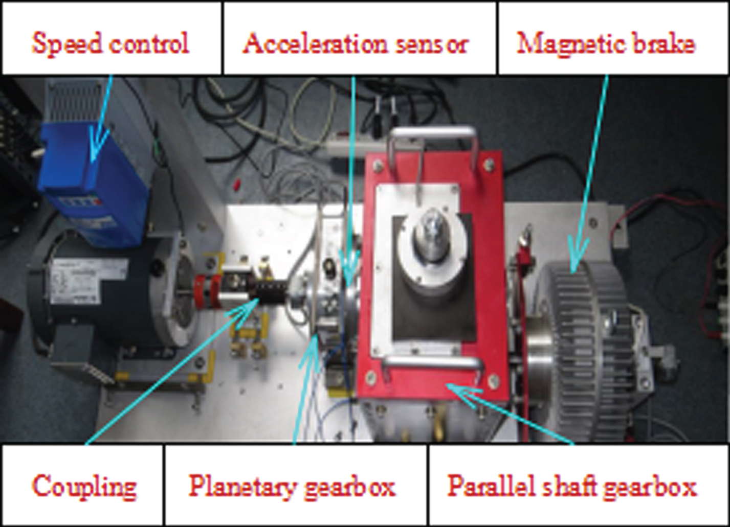
5 Experiment set up and signal acquisition

The effectiveness of the fault diagnosis model for rotating machinery based on OSSLLTSA and TSVM was demonstrated by the simulation experiment of gearbox faults. In real engineering application, gearbox faults account for 80% of transmission system faults and 10% of rotating machinery faults. Therefore, the fault diagnosis for gearboxes is of great importance and engineering application value. In this study, the simulation of operation state of rotating machine was carried out based on one-stage planetary gear box and two-stage parallel shaft gearbox, and the laboratory built gearbox fault simulation experiment table is shown in Fig. 2.

Fig.2

The test point arrangement in gearbox vibration test.

The gearbox test rig mainly consists of speed control device, variable frequency AC drive motor, planetary gear box, second stage parallel shaft gearbox, magnetic brake, etc. The drive motor speed can be adjusted within 0 to 5000 rpm. In this experiment, the test rig is composed of a one-stage planetary gearbox and a two-stage parallel shaft gearbox. In the experiment, the drive motor speed was set to 1200 rpm, the load of magnetic brake was 1.5 pounds, and no radial load was made for the gearbox. The vibration signals were collected by the vibration acceleration sensor installed at the bearing cover of the input end of intermediate shaft, with sampling frequency set at 5 kHz.

A total of 5 kinds of gear states were simulated, namely (1) normal; (2) broken tooth fault; (3) missing tooth fault; (4) tooth surface wear; and (5) synthetic fault, and the main parameters of the experiment are listed in Table 2.

Table 2

The main parameters of the gearbox fault experiment

Parameter/Device	Value/Type
Driving speed	1200 rpm
No. of solar gear teeth	20
No. of planetary gear teeth	40
No. of inner ring gear	100
No. of input gear teeth of parallel shaft gearbox	100
No. of intermediate shaft gear teeth of parallel shaft gearbox	29, 36
No. of output shaft gear teeth of parallel shaft gearbox	90
Acquisition card	NI9234
Acceleration sensor	PCB352C03
Data acquisition system	DP/INV306U
Sampling frequency	5 kHz

The original vibration signals were collected by the acceleration sensors. Figure 3 shows the time domain waveform of the original vibration signals collected by the sensor in different operation states. A number of 120 sets of samples were collected for each state, among which 80 sets were training samples and the rest were used for testing the fault diagnosis model, with the length of each sample being 2048 sampling points.

Fig.3

The time waveform and frequency spectrum of original vibration signals: (a) mixed bearing fault; (b) outer ring fault; (c) missing tooth fault; (d) rolling element fault; and (e) tooth surface wear fault.

6 Experimental results and analysis

6.1 Experiment results

Since the frequency components of the collected original vibration signals are complicated with significant non-linear and non-stationary characters, the original signals were decomposed by WPD by using ‘db8’ wavelet basis on 3 scales, and the selection of wavelet basis can refer to [37]. Then, 8 statistic features in time-frequency domain, 4 AR model parameters, 1 instantaneous amplitude Shannon entropy and 1 wavelet packet decomposition energy were extracted from each sub-band to form the high dimensional fault feature set. In other words, the original high dimensional fault feature set contained 112 fault features, which could characterize faults from multiple aspects, and the original feature set was rich of fault information. Since the original high dimensional fault feature set was inevitably mixed with insensitive and interference features, IKMD-FS was adopted to select fault features, with feature selection results shown in Fig. 4. It is clear that after feature selection, 67 fault features remained in the feature set, the dimension of the feature set still being very high. Moreover, the non-linear coupling relation between fault features also caused the high dimensional feature set to contain a large amount of redundant information. Therefore, after feature selection, the high dimensional fault feature set was then inputted into OSSLTSA algorithm for dimensionality reduction. The objective dimension d was set to 5 for dimensionality reduction, and the neighborhood size k was set to 12. Table 3 shows the low dimensional coordinates of each class of fault samples when the ratio of labeled samples to the total samples is a = 0.4. Inputting the obtained low dimensional fault feature set into a pattern recognition method can realize fault class identification. TSVM was used in this study to establish the fault pattern recognition model. Table 4 lists the diagnosis results of the proposed method based on OSSLLTSA and TSVM. It is clear from Table 4 that the proposed method has advantages in situations where labeled training samples are insufficient. When a = 0.4, the fault recognition accuracy reached 95.5%.

Fig.4

Result of feature set after feature selection.

Table 3

Low-dimensional coordinates of fault samples by using OSSLLTSA

Running state	Sample number No.	Low-dimensional coordinates of fault samples
Normal state	14	(– 0.0875 – 0.0474 – 0.0082 – 0.0070)
	15	(– 0.0888 – 0.0500 – 0.0093 – 0.0040)
	16	(– 0.0869 – 0.0508 – 0.0100 – 0.0032)
Broken tooth fault	14	(– 0.0068 0.0666 0.0332 – 0.04291)
	15	(– 0.0093 0.0624 0.0349 – 0.0471)
	16	(– 0.0074 0.0661 0.0381 – 0.0728)
Missing tooth fault	14	(– 0.0116 0.0433 0.0168 0.0214)
	15	(– 0.0031 0.0416 0.0086 0.0607)
	16	(– 0.0086 0.0466 0.0153 0.0407)
Tooth surface wear	14	(0.0422 0.0014 – 0.1190 – 0.0451)
	15	(0.0417 0.0018 – 0.1174 – 0.0439)
	16	(0.0429 0.0009 – 0.1198 – 0.0460)
Synthetic fault	14	(0.0645 – 0.0697 0.0570 – 0.0089)
	15	(0.0522 – 0.0431 0.0131 – 0.0023)
	16	(0.0652 – 0.0707 0.0612 – 0.0041)

Table 4

The change of fault diagnosis accuracy with ratio of labeled samples a

Ratio of labeled samples (a)	0.2	0.4	0.6	0.8	1.0
Accuracy (%)	94	95.5	97	97.5	98

6.2 Experiment analysis

To further verify the effectiveness of the proposed method, the following comparative experiments were made.

Comparative analysis was made for the effectiveness of different construction methods of high dimensional fault feature sets. For simplicity of analysis, it is assumed in the comparative experiments that all training samples are labeled samples, and KNNC algorithm is adopted for fault diagnosis. Firstly, the necessity and effectiveness of using WPD to preprocess the vibration signals are analyzed. Table 5 lists the diagnosis results of using WPD for preprocessing and those without WPD preprocessing. It is clear from the results that the diagnosis accuracy using original vibration signals for fault feature extraction is 89.5%, while the diagnosis accuracy using the WPD to preprocess vibration signals for fault feature extraction is 94.5%. Moreover, the necessity and effectiveness of feature selection are analyzed. Table 6 lists the fault diagnosis results of using feature selection and those without feature selection. It is clear from Table 6 that feature selection removes the insensitive and interference noise features in the original high dimensional fault feature set. Therefore, the fault diagnosis accuracy using feature selection is higher than that of directly using the original fault feature set.

The effectiveness of OSSLTSA algorithm is analyzed. The fault diagnosis accuracy of OSSLLTSA algorithm is compared with PCA, LLTSA and SLLTSA. KNNC algorithm is adopted for fault diagnosis, and only the labeled samples are used for KNNC training. Table 7 shows the fault diagnosis accuracy after using these dimensionality reduction methods for feature extraction. It is clear from Table 7 that when SLLTSA algorithm is used, the fault diagnosis accuracy with fewer labeled samples is very low. The reason is that SLLTSA algorithm is easy to be trapped in over-learning when labeled training samples are insufficient. Conversely, the fault diagnosis accuracy for LLTSA and PCA is low. Moreover, the fault diagnosis accuracy of PCA is lower than LLTSA. The reason is that PCA is unable to extract the nonlinear structural information contained in data set, while LLTSA has certain structural extraction ability. In addition, by comparing SLLTSA and LLTSA, it can be found that when labeled samples increase to a certain degree, the SLLTSA algorithm outperforms LLTSA. OSSLLTSA is a semi-supervised dimensionality reduction method, which is able to simultaneously extract the structural information of labeled and unlabelled samples, avoiding the over-learning problem of SLLTSA where labeled samples are insufficient and the projection aimlessness of LLTSA in dimensionality reduction. Therefore, the performance of using OSSLTSA for dimensionality reduction is better than using other methods. It is clear from Table 7 that the fault diagnosis accuracy of OSSLTSA is the best among these methods.

The effectiveness of TSVM is compared with SVM and KNNC. In the comparative experiment, the low dimensional fault features extracted by OSLLTSA were the input of pattern recognition algorithms. Table 8 lists the fault diagnosis results of using 3 pattern recognition methods. KNNC is a pattern recognition algorithm based on statistics, with advantages of low computational cost, stable performance, etc. However, when labeled training samples are insufficient, the recognition accuracy of KNNC algorithm decreases. When the ratio of labeled samples is a = 0.2, the recognition accuracy of KNNC is 90%, which is lower than that of SVM and TSVM. SVM is a pattern recognition algorithm based on structural risk minimization, which realizes fault diagnosis by constructing classification hyperplane. However, when labeled samples are insufficient, the classification hyperplane calculated by SVM deviates from the optimal classification hyperplane, causing the over-learning problem of SVM. When the ratio of labeled samples is a = 0.2, the recognition accuracy of SVM is 92%. TSVM is the semi-supervised improvement of SVM, which is able to simultaneously extract the distribution information of labeled and unlabelled training samples, and use the sample distribution information contained in unlabelled samples to modify the classification hyperplane. Therefore, when labeled samples are rare, TSVM is still able to achieve good fault diagnosis results. When the ratio of labeled samples is a = 0.2, the recognition accuracy of TSVM is 94%, which is better than that of KNNC and SVM.

Table 5
Fault diagnosis accuracy with versus without WPD

Whether WP before feature set construction? Dimension d Fault diagnosis accuracy

No 13 89.5%

Yes 112 94.5%

Whether WP before feature set construction?	Dimension d	Fault diagnosis accuracy
No	13	89.5%
Yes	112	94.5%

Table 6

Running identification rate with versus without feature selection

Whether feature selection before feature set construction?	Dimension d	Identification accuracy
No	112	88%
Yes	67	94.5%

Table 7

The change of fault diagnosis accuracy with ratio of labeled samples a

Ratio of labeled samples (a)	0.2	0.4	0.6	0.8	1
PCA (%)	68	71	74	74.5	75
LLTSA (%)	78.5	81.5	83	84	84.5
SLLTSA (%)	73.5	85	91	93	94.5
OSSLLTSA (%)	88	91	93.5	94	94.5

Table 8

The change of running state identification accuracy with ratio of labeled samples a

Proportion of labeled samples (a)	0.2	0.4	0.6	0.8	1
KNNC (%)	88	91	93.5	94	94.5
SVM (%)	90.5	93	95	96.5	98
TSVM (%)	94	95.5	97	97.5	98

7 Conclusions

A fault diagnosis model was proposed using OSSLTLTSA for feature extraction and TSVM for fault identification. According to the experimental results, some conclusions are summarized as follows:

The features extracted from sub-bands decomposed by WPD can characterize fault better than those extracted from original signals, and feature selection based on IKDM-FS can remove insensitive features or even interference feature from the feature set.

OSSLTSA can is able to simultaneously extract the structural information from both labeled and unlabelled samples, thus overcoming the drawback of unsupervised manifold learning that it is aimless in feature extraction. Dimensionality reduction by OSSLLTSA can well extract the sensitive fusion feature for fault diagnosis.

TSVM is able to modify the model and improve fault classification accuracy by fully using the fault information in unlabelled samples. The effectiveness of the proposed method was verified by a fault diagnosis test in a gearbox.

Footnotes

Acknowledgments

This project was supported by National Natural Science Foundation of China (Grant Nos. 51705059, 51605065), by Scientific and Technological Research of Chongqing Municipal Education Commission (Grant Nos. KJ1600428, KJ1600443).

References

Ribrant

, Bertling

, Survey of failures in wind power systems with focus on Swedish wind power plants during 1997-2005, Power Engineering Society General Meeting, 2007. IEEE. IEEE (2007), 1–8.

Cerrada

, Sánchez

, Li

, ., A review on data-driven fault severity assessment in rolling bearings, Mechanical Systems & Signal Processing99 (2018), 169–196.

Shen

, Wang

, Kong

, ., Fault diagnosis of rotating machinery based on the statistical parameters of wavelet packet paving and a generic support vector regressive classifier, Measurement Journal of the International Measurement Confederation46 (4) (2013), 1551–1564.

Wang

, K-nearest neighbors based methods for identification of different gear crack levels under different motor speeds and loads: Revisited, Mechanical Systems & Signal Processings70-71 (2016), 201–208.

Pan

, Chen

, Li

, Bearing performance degradation assessment based on lifting wavelet packet decomposition and fuzzy c-means, Mechanical Systems & Signal Processing24 (2) (2010), 559–566.

Ding

X.X.

, Qing-Bo

H.E.

, Machine fault diagnosis based on WPD and LPP, Journal of Vibration & Shock33 (3) (2014), 89–93.

, Chen

, Gui

, ., Adaptive PCA based fault diagnosis scheme in imperial smelting process, Isa Transactions53 (5) (2014), 1446–1455.

Jolliffe

, Principal Component Analysis. Springer-Verlag; 2002.

Hyvarinen

, Oja

, Independent component analysis: Algorithms and applications, Neural Networks13 (425) (2000), 411–430.

10.

Rweis

S.T.

, Saul

L.K.

, Nonlinear dimensionality reduction by locally linear embedding, Since290 (2000), 2323–2326.

11.

Tenenbaum

J.B.

, De Silva

and Langford

J.C.

, A global geometric framework for nonlinear dimensionality reduction, Science290 (5500) (2000), 2319–2323.

12.

Zhang

Z.Y.

, Zha

H.Y.

, Principal manifolds and nonlinear dimensionality reduction via tangent space alignment, Society for Industrial and Applied Mathematics Journal of Scientific Computing26 (2004), 313–338.

13.

, Cai

, Yan

, ., Neighborhood preserving embedding, Tenth IEEE International Conference on Computer Vision. IEEE Computer Society (2005), 1208–1213.

14.

Wang

G.F.

, Yang

Y.W.

, Zhang

Y.C.

, ., Vibration sensor based tool condition monitoring using support vector machine and locality preserving projection, Sensors & Actuators A Physical209 (Complete) (2014), 24–32.

15.

Zhang

, Yang

, Zhao

, ., Letters: Linear local tangent space alignment and application to face recognition, Neurocomputing70 (7) (2007), 1547–1553.

16.

Cheng

, Liu

, Lu

, ., Supervised kernel locality preserving projections for face recognition, Neurocomputing67 (1) (2005), 443–449.

17.

Wang

, Wang

, Zhang

, ., Face recognition using marginal discriminant linear local tangent space alignment, International Conference on Intelligent System Design & Engineering Application. IEEE Computer Society (2012), 1418–1421.

18.

, Wang

, Tang

, ., Life grade recognition method based on supervised uncorrelated orthogonal locality preserving projection and K-nearest neighbor classifier, Neurocomputing138 (138) (2014), 271–282.

19.

Shi

, Liu

, Zhang

, ., Kernel local linear discriminate method for dimensionality reduction and its application in machinery fault diagnosis, Shock and Vibration, 2014, (2014-2-27)2014 (20) (2014), 1–11.

20.

X.P.

, Yu

X.G.

, Novel text classification based on k-nearest neighbor, in: Proceedings of Sixth International Conference on Machine learning Cyber-netics, HongKong, China, (2007), 3425–3430.

21.

Azadeh

, Saberi

, Kazem

, ., A flexible algorithm for fault diagnosis in a centrifugal pump with corrupted data and noise based on ANN and support vector machine with hyper-parameters optimization, Appl SoftComput3 (2013), 1478–1486.

22.

Ukil

, Support vector machine, Computer Science1 (4) (2002), 1–28.

23.

Hsu

C.C.

, Chen

M.C.

, Chen

L.S.

, Intelligent ICA-SVM fault detector for non-Gaussian multivariate process monitoring, Expert Systems with Applications37 (4) (2010), 3264–3273.

24.

Liu

, Yang

, Zhang

, ., Time-frequency atoms-driven support vector machine method for bearings incipient fault diagnosis, Mechanical Systems & Signal Processing75 (2016), 345–370.

25.

Shen

, Chen

, Zhang

, ., A novel intelligent gear fault diagnosis model based on EMD and multi-class TSVM, Measurement45 (1) (2012), 30–40.

26.

Lei

, Zuo

M.J.

, He

, ., A multidimensional hybrid intelligent method for gear fault diagnosis, Expert Systems with Applications37 (2) (2010), 1419–1430.

27.

Chen

F.F.

, Tang

B.P.

, Song

, ., Multi-fault diagnosis study on roller bearing based on multi-kernel support vector machine with chaotic particle swarm optimization, Measurement47 (2014), 576–590.

28.

Bafroui

H.H.

, Ohadi

, Application of wavelet energy and Shannon entropy for feature extraction in gearboxfault detection under varying speed conditions, Nerocomputing133 (2014), 437–446.

29.

Wang

G.F.

, Liu

and Cui

Y.H.

, Clustering diagnosis of rolling element bearing fault based on integratedAutoregressive/Autoregressive Conditional Heteroscedasticity model, Journal of Sound and Vibration331 (2012), 4379–4387.

30.

, Tang

, Liu

, ., Multi-fault diagnosis for rotating machinery based on orthogonal supervised linear local tangent space alignment and least square support vector machine, Neurocomputing157 (2015), 208–222.

31.

Zu-Qiang

S.U.

, Tang

B.P.

, Yao

J.B.

, Fault diagnosis method based on sensitive feature selection and manifold learning dimension reduction, Journal of Vibration & Shock33 (3) (2014), 70–75.

32.

Cai

Z.Y.

, Yu

J.G.

, Li

X.P.

, ., Feature selection algorithm based on kernel distance measure, Pattern Recognition & Artificial Intelligence23 (2) (2010), 235–240.

33.

Zhang

S.Q.

, Enhanced supervised locally linear embedding, Pattern Recognition Letters30 (2009), 1208–1218.

34.

Wang

, Jiang

W.X.

, Guo

, Extended local tangent space alignment for classification, Neurocomputing77 (2012), 261–266.

35.

Deng

C.A.I.

, Xiaofei

H.E.

, Jiawei

H.A.N.

, ., Orthogonal Laplacian faces for face recognition, IEE Transactions of Image Processing11 (2006), 3608–3614.

36.

Weihua

L.I.

, Liu

, Gear incipient fault diagnosis using graph theory and transductive support vector machine, Journal of Mechanical Engineering46 (23) (2010), 82.

37.

Wang

, Xu

, Liang

, . Detection of weak transient signals based on wavelet packet transform and manifold learning for rolling element bearing fault diagnosis, Mechanical Systems and Signal Processing (2015), 259–276.

Fault diagnosis based on orthogonal semi-supervised LLTSA for feature extraction and Transductive SVM for fault identification

Abstract

Keywords

1 Introduction

2 Feature extraction by semi-supervised LLTSA

2.1 High-dimensional fault feature set

2.1.1 Original fault feature set extraction

2.1.2 Fault feature selection

2.2.1 Brief review of LLTSA

6.1 Experiment results

Table 5 Fault diagnosis accuracy with versus without WPD Whether WP before feature set construction? Dimension d Fault diagnosis accuracy No 13 89.5% Yes 112 94.5%

Footnotes

Acknowledgments

References

Table 5
Fault diagnosis accuracy with versus without WPD

Whether WP before feature set construction? Dimension d Fault diagnosis accuracy

No 13 89.5%

Yes 112 94.5%