Auxiliary-model-based domain adaptation for reciprocating compressor diagnosis under variable conditions

Abstract

Machine learning is widely used for fault diagnosis research. In general, most models used for fault diagnosis are based on the same data distribution, whereas applying equipment to practical productions and operations are mostly done under variable conditions. This often produces changes in data distribution and makes the model unavailable. As one of the most commonly used pieces of equipment in industry, a reciprocating compressor operates under various operating conditions (e.g., variable speed), which may produce changes in data distribution. Thus, the current model established under stable conditions is no longer applicable for fault diagnosis under variable conditions. To solve this problem of variable conditions, a model should be established that 1) reduces the differences caused by different operating conditions as much as possible, and 2) learns representative fault features under different working conditions. Thus, a new strategy that employs an auxiliary model is proposed that combines a convolutional neural network (CNN) and a marginalized stacked denoising autoencoder (mSDA). In our method, 1) the pre-training model CNN is used for feature learning, and 2) the learned features are transformed by mSDA to eliminate data distribution differences between different conditions. A statistical measure based on kernel maximum mean discrepancy is used to evaluate the differences across different domains. Experimental results of a reciprocating compressor under different operating conditions demonstrate that the proposed method can learn class sensitive features and eliminate differences with changing working conditions. It also obtains higher classification accuracy for reciprocating compressor diagnosis under different working conditions.

Keywords

Auxiliary model domain adaptation reciprocating compressor fault diagnosis variable conditions

1 Introduction

With the development of machine learning, the technology for condition monitoring and fault diagnosis has been studied in depth and widely applied to ensure normal machine operation [1 –3]. The model based on supervised and unsupervised machine learning methods has given rise to accurate fault classification. Normally, most of these models are based on the same distribution of training and test data. The operative mode of equipment in practical production is variable, which creates changes in data distribution. These differences will affect the diagnostics of the model and can even lead to model failure. For example, as one of the most commonly used pieces of equipment in industry, a reciprocating compressor operates under various operating conditions and is diagnosed by applying a vibrational signal. Here, the distribution of collected data changes with the various motor rotating speeds. The training data for building a classifier might be collected under conditions involving a specific rotating speed, and a practical application must be able to diagnose a compressor system under different rotating speeds. As a result, a model built with training data (i.e., the source domain) cannot be directly applied to a target situation (i.e., a target domain). Therefore, a model established using a traditional method for diagnosis will be unable to detect the defects in a compressor accurately under variable conditions.

Domain adaptation [4, 5] establishes a learning model that can reduce changes in data distribution between different but related domains and can learn features from one domain to another. Domain adaptation is widely used in voice, image recognition, and text classification [6 –8]. As one of the most preeminent methods of domain adaptation, the marginalized stacked denoising autoencoder (mSDA) has shown excellent performance in numerous fields [9]. It can learn common features from cross domains by reconstructing corrupted data. This enables the data distribution to be as uniform as possible and eliminates data distribution changes caused by operating changes.

However, simply eliminating differences cannot guarantee high classification accuracy for diagnosis because not only are categories neglected but also the model must be able to learn specific features generated by different categories. A convolutional neural network (CNN) takes advantage of learning features that are more sensitive to categories. It accomplishes this in a supervised learning manner. CNN is the first successful multi-layer structural algorithm [10], and its unique features (e.g., using a local connection, employing weight sharing and sub-sampling, etc.) greatly simplify the complexity of model training. In the field of machine learning, particularly in the field of machine vision, CNN has become a focus of research.

To solve the aforementioned problems, realize domain adaption, and synthesize distinguishable features, a new strategy called auxiliary-model-based domain adaptation (AMDA) is proposed in this study to enhance the ability of learning fault sensitive features and eliminate changes in data distribution caused by different working conditions. First, as an auxiliary pre-training model, CNN is combined with mSDA to learn fault sensitive features and eliminate data distribution differences between different conditions. Second, the features learned by this complex model are used as input to train a classifier. Support vector machine (SVM) is employed in this study as well. An experiment with a compressor is conducted to analyze and validate the performance of the proposed method. In our experiment, different speed cases refer to different but related domains. Our method proves to be effective when compared to some traditional machine-learning methods.

This study presents domain adaptation in the field of machinery fault diagnosis. The remainder of this paper is organized as follows. Section 2 provides descriptions of the theoretical framework including the mSDA method and CNN model. Section 3 discusses the proposed method in detail. In Section 4, experimental results on the reciprocating compressor are given in order to validate our proposed method’s ability to perform reciprocating compressor diagnosis under variable conditions. Comparative results are also given in Section 4. The conclusion of this study is provided in Section 5.

2 Theoretical framework

2.1 Marginalized stacked denoising autoencoders

The mSDA [9] is a modified version of the stacked denoising autoencoder (SDA) [11], which alleviates differences in distribution by transforming data into another subspace in a manner such that corrupted data are rebuilt.

The basic building block is a one-layer denoising autoencoder, which is called a marginalized denoising autoencoder (mDA). First, inputs x₁, …, x_n from source and target domains D = D_S ∪ D_T are corrupted by random feature removal, and each feature is set to 0 with a probability of P ≥ 0. Unlike in the two-level encoder and decoder in SDA, the corrupted inputs are reconstructed with a single mapping W: R^d → R^d, which minimizes the squared reconstruction loss: $\frac{1}{2 n} \sum_{i = 1}^{n} {∥ x_{i} - W {\tilde{x}}_{i} ∥}^{2}$ (1) where x_i is the raw input and ${\tilde{x}}_{i}$ is the corrupted version of x_i.

Equation (1) is based on those features of each input that are corrupted randomly. To reduce the variance, multiple passes over the training set are performed, each time with a random corruption. The mapping W can be obtained by minimizing the overall squared loss: $L_{sq} (W) = \frac{1}{2 mn} \sum_{j = 1}^{m} \sum_{i = 1}^{n} {∥ x_{i} - W {\tilde{x}}_{i, j} ∥}^{2}$ (2) where ${\tilde{x}}_{i, j}$ represents the jth corrupted version of the original input x_i.

Therefore, the design matrix X = [x₁, …, x_n] ∈ R^d×n and its m-times repeated matrix $\bar{X} = [X, \dots, X]$ are defined. In addition, the corrupted version of $\bar{X}$ is denoted as $\tilde{X}$ . Then, the loss in (1) is reduced to: $L_{sq} (W) = \frac{1}{2 mn} tr [(\bar{X} - W \tilde{X})^{T} (\bar{X} - W \tilde{X})]$ (3)

Then, to solve (3), the closed-form solution for ordinary least squares is used: $W = {PQ}^{- 1} with Q = \tilde{X} {\tilde{X}}^{T} and P = \bar{X} {\tilde{X}}^{T}$ (4)

If m becomes very large, the matrices P and Q can be substituted with their expected values according to the weak law of large numbers. When we focus on a limit case, where m→ ∞, the expectations of Q and P can be obtained, and W can be expressed as: $W = E [P] E [Q]^{- 1}$ (5)

The next task is to compute the expectations of these two matrices. First, we focus on: $E [Q] = \sum_{i = 1}^{n} E [{\tilde{x}}_{i} {\tilde{x}}_{i}^{T}]$ (6)

If both features α and β are not removed during the corruption process, the probability that an off-diagonal element in the matrix ${\tilde{x}}_{i} {\tilde{x}}_{i}^{T}$ will not be destroyed is (1 - p) ². However, the diagonal entries may be destroyed with a probability of 1 - p. A vector q = [1 - p, …, 1 - p, 1] ^T ∈ R^d+1 exists, where q_α represents the probability that a feature α is uncorrupted. In addition, the constant feature is never corrupted that is q_d+1 = 1. If the scatter matrix of the original uncorrupted input is defined as S = XX^T, the expectation of the matrix Q would be expressed as: $E [Q]_{α, β} = {\begin{matrix} S_{α β} q_{α} q_{β} & if α \neq β \\ S_{α β} q_{α} & if α = β \end{matrix}$ (7)

Similarly, the expectation of P in closed form is derived as E [P] _αβ = S_αβq_β.

With the help of these expectation matrices, the reconstruction mapping W is calculated directly from the closed equation without specifying the construction of each single corrupted input ${\tilde{x}}_{i}$ . Like SDA, several mDA layers can be stacked by providing the output of the (t - 1) ^th mDA as the input into the tth mDA. The training is performed greedily layer by layer: each map W^t is learned (in closed form) to reconstruct the previous mDA output h^t-1 from all possible forms of corruption. Denote the output of the tth mDA as h^t and the original input as h⁰ = x so that the output of the tth layer becomes h^t = tanh(W^th^t-1). The construction is shown as Fig. 1.

Fig.1

Construction of mSDA.

2.2 Convolutional neural network

A typical CNN is composed of two kinds of deep hidden layers: convolutional and subsampling. Structurally speaking, these layers are arranged alternately after data for feature extraction and dimensionality reduction are input, respectively.

The convolutional layers consist of a series of convolutional kernels, which are equivalent in function to weight templates. As the response and extracted features of the convolutional layers, the weighted sum of the data is calculated and output by the convolutional kernels through sliding on the input data. Therefore, the aforementioned operation is known as convolution and can be defined as follows:

$\begin{matrix} C & = & conv (f, w) = f (x, y) \times w (s, t) \\ = & \sum_{s = - a}^{a} \sum_{t = - b}^{b} w (s, t) \times f (x - s, y - t) \end{matrix}$ (8) where f (x, y) and w (s, t) are the input map and convolutional kernel, respectively. Clearly, each kind of convolutional kernel can be used only with a particular feature such as oriented edges, colors, and corners [12]. To extract various features, several convolutional kernels usually exist simultaneously in a convolutional layer. Therefore, assuming M output maps exist in a k layer and N convolutional kernels in a k + 1 layer, the value is:

$\begin{matrix} C_{ji}^{k + 1} = conv (f_{i}^{k}, ω_{j}^{k + 1}) \\ i = 1, 2 \dots M; j = 1, 2 \dots N \end{matrix}$ (9)

Then, the output (or feature) maps of the k + 1 layer can be calculated by: $y_{j}^{k + 1} = s (\sum_{i \in M_{i}} C_{ji}^{k + 1} + b_{j}^{k + 1}); j = 1, 2 \dots N$ (10) where s is the activation function and $b_{j}^{k + 1}$ is the bias of the j-th convolutional kernel. M_i denotes the selection of input maps, which is performed through a local connection.

Usually, subsampling layers are inserted behind one or several convolutional layers to solve the superabundant dimensions of feature maps produced by continuous convolution. In a concrete operation, the feature maps outputted by the convolutional layers are divided into several regions and no overlap exists between them. Statistics related to each region are used to replace original values. Therefore, assuming the subsampling layer is a k + 2 layer, the detailed subsampling operation is defined as:

$\begin{matrix} S_{j}^{k + 1} = β_{j}^{k + 2} down (y_{j}^{k + 1}) + b_{j}^{k + 2} \\ j = 1, 2 \dots N \end{matrix}$ (11) where down denotes the sub-sampling computation, and $β_{j}^{k + 2}$ and $b_{j}^{k + 2}$ represent the weight matrix and bias, respectively. Then, the features maps of the subsampling layer are as follows: $a_{j}^{m + 2} = f (S_{j}^{m + 2}); j = 1, 2 \dots N$ (12) where f is the activation function.

3 Auxiliary-model-based domain adaptation

Different working conditions and faults both generate distributions changes of vibrational signals. The original mSDA method may eliminate differences caused not only by different domains but also by different classes. In Chen [9], raw input data and the learned feature were combined as a new presentation. The new presentation would retained both the class and domain features. However, this may not work well for vibration data because of the interference of vibration noises and other fault-free information. Therefore, we design an auxiliary model by combining CNN and mSDA. A schematic of the proposed method is given as Fig. 2. First, a pre-training model is established by CNN, which focuses on learning the sensitive features generated by faults and on reducing the dimension. Then, mSDA is used to eliminate data distributions differences between different conditions by recovering corrupted data and transforming the data into another subspace. For lower dimensions and fewer parameters, the last layer output would be the ultimate feature learned by the proposed model.

Fig.2

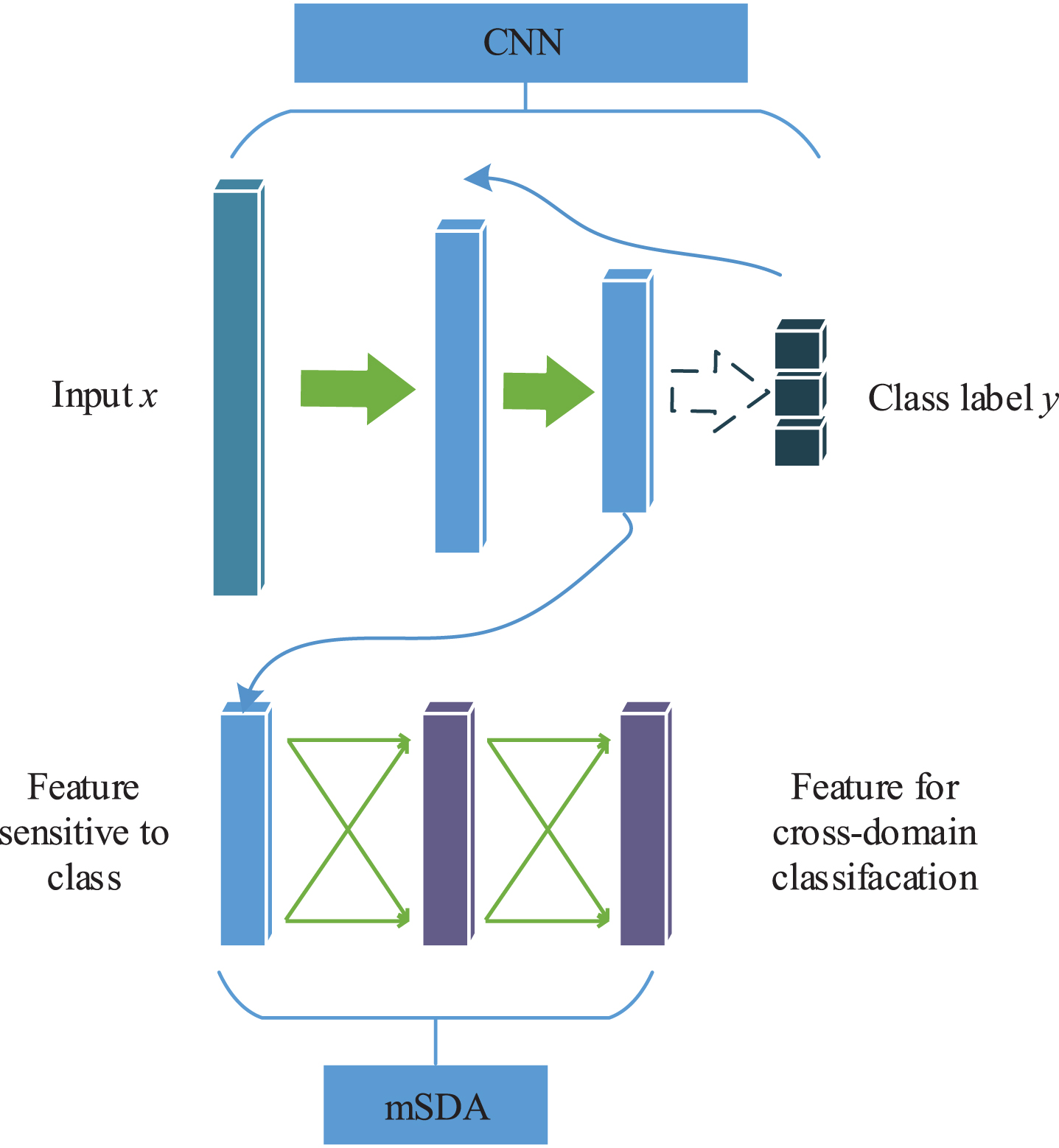
Schematic of the proposed model.

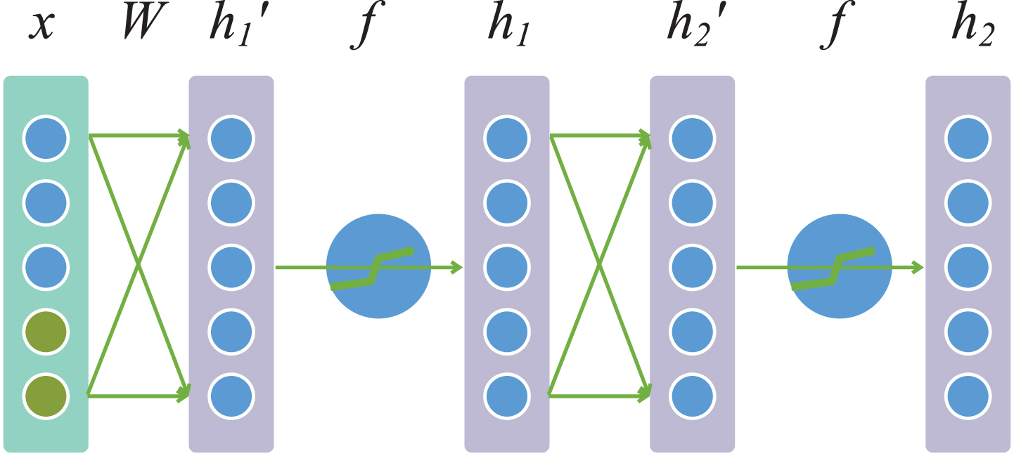
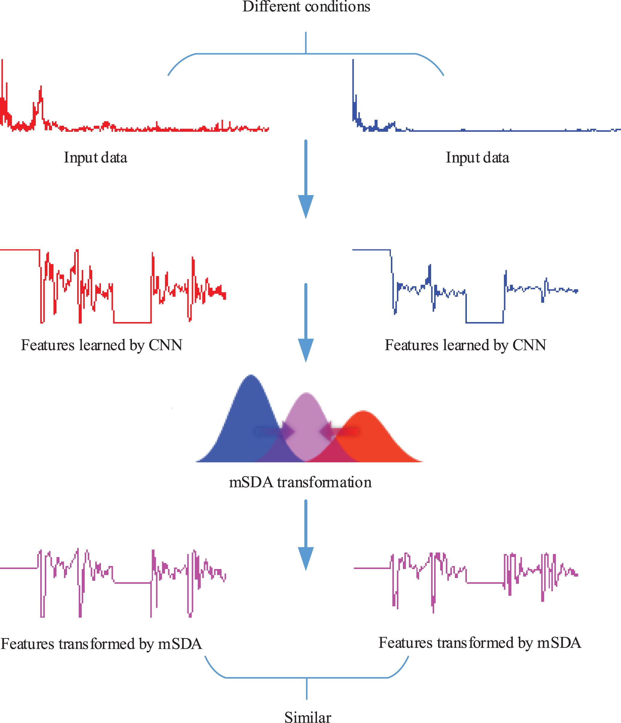
Therefore, CNN as a pre-training model is applied to help mSDA learn class-sensitive features, which are in a lower dimension. Then, these lower dimension features, as the original input x of mSDA, are used to calculate the mapping W. This calculation is given by (5–7). The output h can be obtained through the function h = tanh(Wx). The training is performed greedily layer by layer. The output h^t-1 of the t - 1^th layer is the tth layer input. Therefore, the output of the tth layer becomes h^t = tanh(W^th^t-1). As a result of mSDA transformation, features under different working conditions would be similarly distributed. The destruction process of each step during feature learning is shown in Fig. 3.

Fig.3

Destruction process of each step during feature learning.

Features learned by the proposed model indicate both the differences between and relevance of the source and target domains. This learning process is necessary to achieve a higher classification for fault diagnosis under different working conditions.

The specific implementation process is shown in Fig. 4. First, fast fourier transform (FFT) is applied to obtain the corresponding frequency amplitude of each signal sample. A min-max normalization method is used to transform the data into [0, 1]. Next, CNN is used to learn the fault sensitive features in a supervised learning manner. Then, mSDA is employed to eliminate the data distribution differences between different working conditions. The features learned by the model are used as the input of the classifier. Finally, SVM is used to train a classifier. We believe that the proposed model can be applied to different conditions. Therefore, the features learned under one set of working conditions are used as training data. The features learned under another set of conditions are used as testing data.

Fig.4

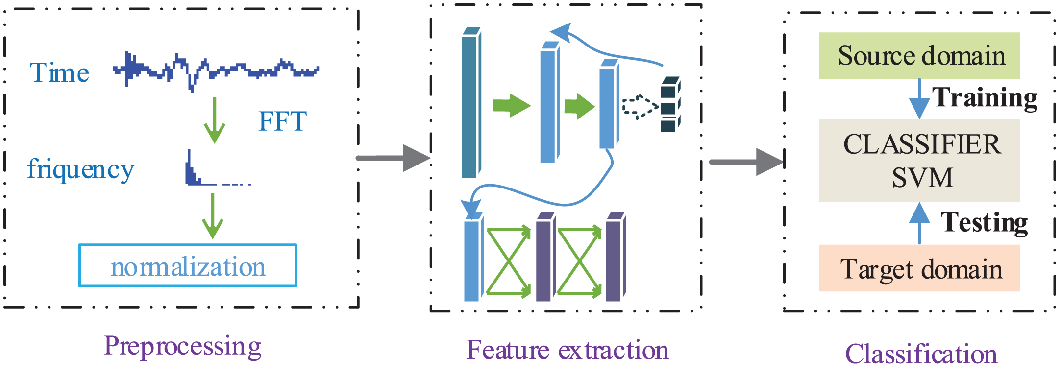
Flow of the training procedure for the proposed model.

CNN learns the specific features of each fault category by extracting a deep hierarchical representation in a supervised manner, and mSDA learns the features of different domains in the shared feature space through spatial transformation. Thus, this complex model can eliminate differences in the distribution of data derived from the source and target domains, and simultaneously learn features accessibility for classification.

4 Experiments

4.1 Experimental setup and dataset

In this study, experimental data collected from a Bently Nevadatrademark RCK-1 Reciprocating Compressor Kit were used to analyze and verify the proposed method. The compressor kit was designed to be an accurate, small-scale representation of a single-cylinder, dual-acting industrial reciprocating compressor, as shown in Fig. 5. Its machine fault capability allows us to induce a drive-train fault condition at the crank/connecting rod interface.

Fig.5

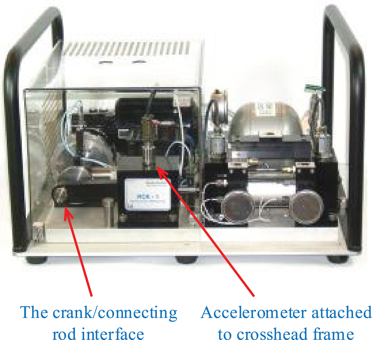
Bently Nevadatrademark RCK-1 Reciprocating Compressor Kit.

The samples under each set of operating conditions (rpm: 80/100/120) were collected through an accelerometer attached to a crosshead frame at a sampling rate of 20,000 Hz, and each condition of rotational speed was regarded as a related but still different domain. There were 200 samples in each domain, including 100 normal samples and 100 drive-train fault samples. The length of each sample was 2000 points.

4.2 Experimental evaluation

Each signal sample was processed by FFT to obtain the single-sided corresponding frequency amplitude. The dimension of the transformational data was 1000 points, which was half of the sample length. The normalized data in the last step were taken as the final input for the model.

In the model, new features were generated by combining CNN and mSDA and used as input data of the classifier. One of the three shaft speeds (80/100/120), which represented the source domain data, was used to train a classifier by SVM, and the other two, which represented target domain data, were used for testing only. Classification results from our model were compared with those from the traditional machine learning methods, including SVM, principal component analysis (PCA), deep belief networks (DBN), CNN, and mSDA are shown in Table 1.

Table 1
Classification results of different operating conditions

Training rpm 80 rpm 100 rpm 120 Mean

Testing rpm 100 rpm 120 rpm 80 rpm 120 rpm 80 rpm 100 Acc.

SVM 74.5 66 71.5 68 59 58 66.2

PCA-SVM 72.5 69 71.5 69 60 65 67.8

DBN 71 64 57.5 60 61.5 58 62

DBN-SVM 69.5 58.5 50 50 58 59 57.5

CNN 48.5 41.5 56.5 46.5 53.5 72.5 53.2

mSDA-SVM 75.5 68 77.5 71.5 72 75.5 73.3

AMDA 83 78.5 91.5 76.5 80.5 80 81.7

Training	rpm 80	rpm 100	rpm 120	Mean
SVM	74.5	66	71.5	68	59	58	66.2
PCA-SVM	72.5	69	71.5	69	60	65	67.8
DBN	71	64	57.5	60	61.5	58	62
DBN-SVM	69.5	58.5	50	50	58	59	57.5
CNN	48.5	41.5	56.5	46.5	53.5	72.5	53.2
mSDA-SVM	75.5	68	77.5	71.5	72	75.5	73.3
AMDA	83	78.5	91.5	76.5	80.5	80	81.7

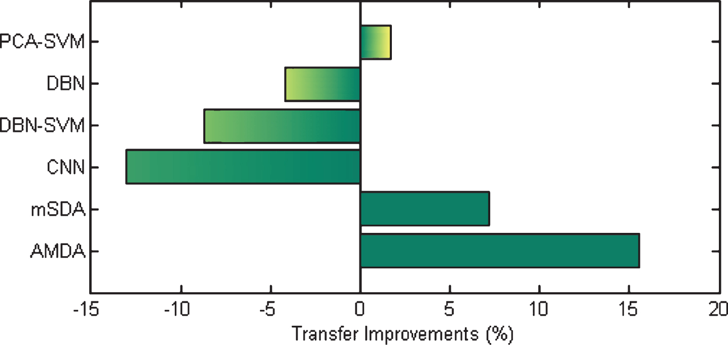
An evaluation metric was used to show improvement in the various methods. This was defined as the difference in classification accuracy between a compared method and the baseline approach (SVM in this study). The improvement results are shown in Fig. 6. Average improvement results of various methods are shown in Fig. 7.

Fig.6

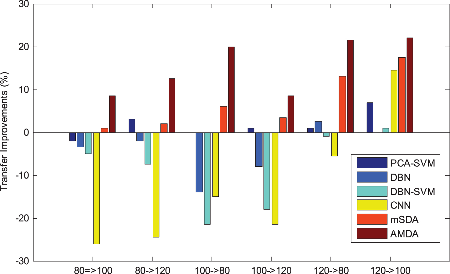
Improvements of various methods.

Fig.7

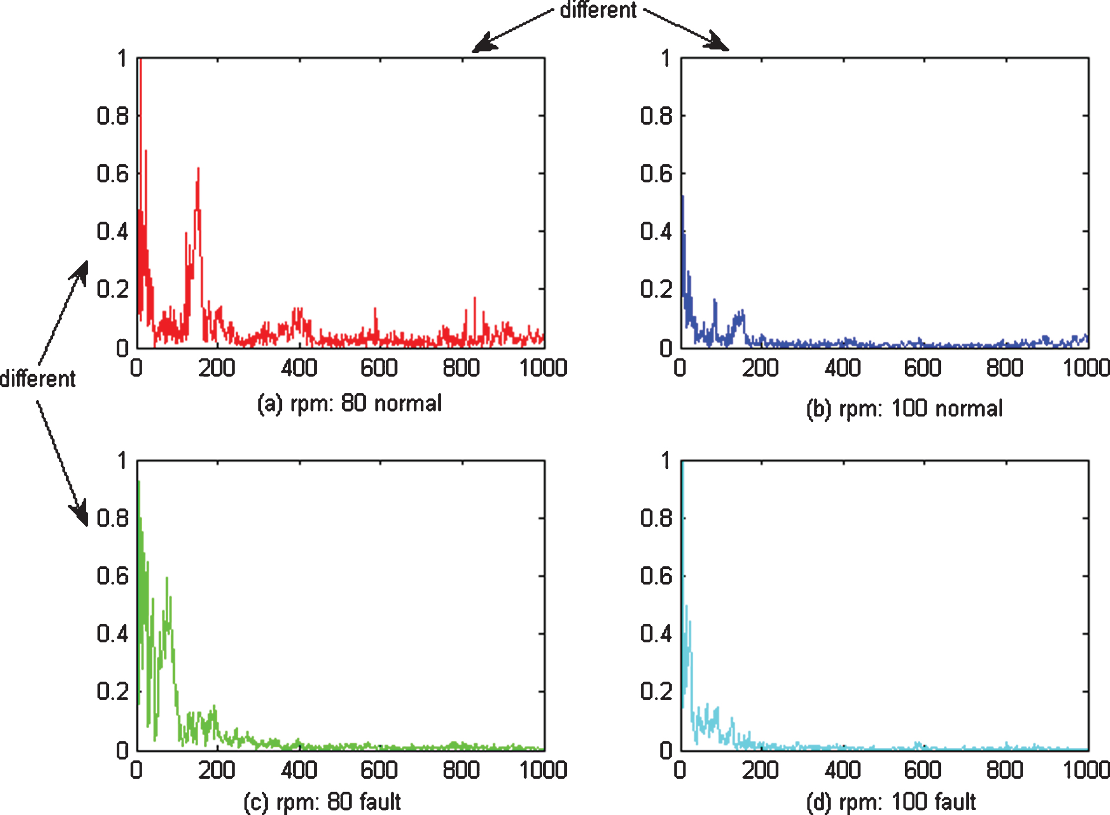
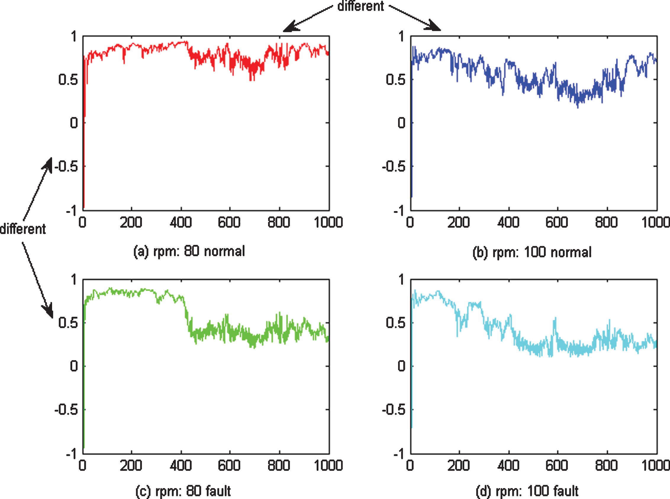
Input data under different conditions and classes.

As shown in Table 1, the proposed method obtained a higher classification accuracy than did the other methods generally, particularly for that of rpm 80-100, rpm 100-80, and rpm 120-80. The results, as shown in Figs. 6 and 7, reveal the effectiveness of the proposed model, which indicates the obvious advantage our model possessed.

The process data under different working conditions (rpm: 80/100) were selected to show the feature differences when using the proposed and traditional methods.

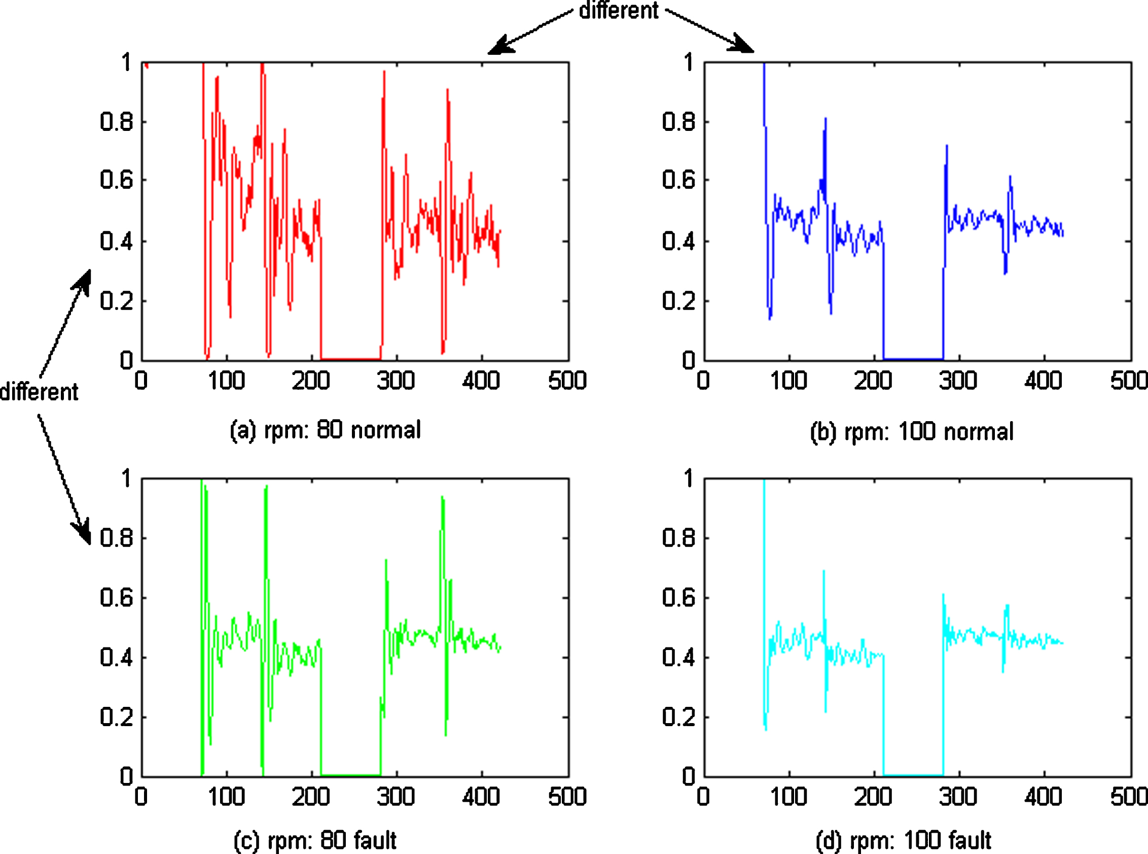
As shown in Fig. 8, the data under different conditions (rpm: 80/100) and different classes (normal/fault) were all different, as were the features learned by mSDA and CNN, as shown in Figs. 9 and 10. The features learned by AMDA under different conditions look similar, but are in fact different, between classes, as shown in Fig. 11.

Fig.8

Features learned by mSDA under different conditions and classes.

Fig.9

Average improvements of various methods.

Fig.10

Features learned by CNN under different conditions and classes.

Fig.11

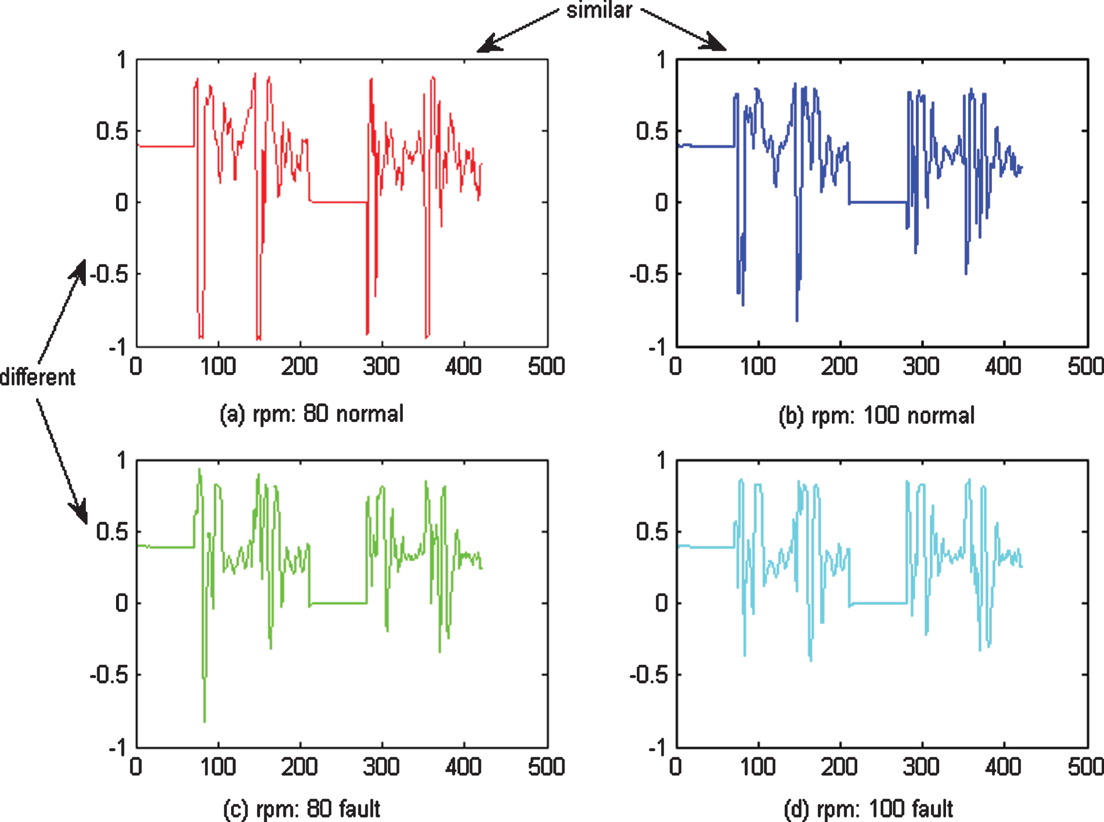
Features learned by AMDA under different conditions and classes.

Another assessment criterion, the kernel maximum mean discrepancy (KMMD) [13], was applied to analyze the divergence indicator of features. Data derived from two working conditions (rpm 80/100) were chosen for the test. Considering about various fault types and working conditions, the discrepancy are calculated respectively when they are in: 1) the two different classes but the same working conditions; 2) the same class but different working conditions. The raw data were compared with the data processed by mSDA. The results are shown in Table 2.

Table 2

KMMD results of different operating conditions

Dataset	Raw data	mSDA	AMDA
80-nomal-80-fault	0.0503	0.0713	0.0717
80-normal-100-normal	0.0588	0.0658	0.0382
80-normal-100-fault	0.0586	0.0744	0.0716
100-normal-100-fault	0.0923	0.0984	0.0817
80-fault-100-fault	0.0764	0.0877	0.0666
100-normal-80-fault	0.1116	0.1228	0.948

As shown in Table 2, the proposed method reduced the discrepancy related to the same class but different conditions.

5 Conclusion

This study presented a strategy, AMDA, for feature presentation of domain adaptation. The practical model based on this strategy combined CNN with mSDA. First, the pre-training model CNN was used for feature learning. Then, the learned features were transformed by mSDA to eliminate data distribution differences between different conditions. The proposed method can learn in a supervised manner the features that are more sensitive to categories of respective domains. The method proved to be useful for classifying cross domains by eliminating cross-domain data distribution differences through mSDA.

Datasets from a reciprocating compressor under different operating conditions were used in experiments and the results revealed that the proposed model yielded a higher classification accuracy than did the traditional models. Feature analysis results firmly validated the effectiveness of the proposed model in successfully eliminating differences generated by different working conditions and in learning fault sensitive features.

Footnotes

Acknowledgments

This research acknowledges the financial support provided by National Key Research and Development Program of China (No. 2017YFC0805803) and National Natural Science Foundation of China (No. 51674277).

References

Tian

, Ma

, Lu

, Wang

, Rolling bearing fault diagnosis under variable conditions using LMD-SVD and extreme learning machine, Mechanism and Machine Theory90 (2015), 175–186.

Yin

, Zhao

, Fault diagnosis network design for vehicle on-board equipments of high-speed railway: A deep learning approach, Engineering Applications of Artificial Intelligence56 (2016), 250–259.

Shao

, Jiang

, Zhao

, Wang

, A novel deep autoencoder feature learning method for rotating machinery fault diagnosis, Mechanical Systems and Signal Processing95 (2017), 187–204.

Daume

, Marcu

, Domain adaptation for statistical classifiers, Artificial Intelligence Research26 (2006), 101–126.

David

S.B.

, Blitzer

, Crammer

, Pereira

, Analysis of representations for domain adaptation, Neural Information Processing Systems, Cambridge: MIT Press, (2006), pp 137–144.

Pan

S.J.

, Tsang

I.W.

, Kwok

J.T.

, Yang

, Domain adaptation via transfer component analysis, IEEE Transactions on Neural Networks22 (2011), 199–210.

Chu

W.S.

, Torre

F.D.L.

, Cohn

J.F.

, Selective transfer machine for personalized facial action unit detection, IEEE Comput Soc Conf Comput Vis Pettern Recognit (2013), 3515–3522.

Long

, Wang

, Ding

, Sun

, Yu

P.S.

, Transfer joint matching for unsupervised domain adaptation, IEEE Comput Soc Conf Comput Vis Pettern Recognit (2014), 1410–1417.

Chen

, Xu

, Weinberger

, Sha

, Marginalized Denoising Autoencoders for Domain Adaptation, International Conference on Machine Learning, Edinburgh Scotland, UK, 2012.

10.

Vincent

, Larochelle

, Bengio

, , Extracting and composing robust features with denoising autoencoders, International Conference on Machine Learning, ACM, (2008), pp 1096–1103.

11.

Vincent

, Larochelle

, Lajoie

, Bengio

, Manzagol

P.A.

, Stacked denoising autoencoders: Learning useful representations in a deep network with a local denoising criterion, The Journal of Machine Learning Research11 (2010), 3371–3408.

12.

Ducottet

String representations and distances in deep Convolutional Neural Networks for image classification, Elsevier Science Inc, 2016.

13.

Borgwardt

, Gretton

, Rasch

, Kriegel

H.-P.

, Schoelkopf

, Smola

, Integrating structured biological data by Kernel Maximum Mean Discrepancy, Bioinformatics22(14) (2006), 1–9.