Gear fault diagnosis based on recurrence network

Abstract

Vibration signals generated from gears often exhibit nonlinearity. Characterization of such signals using nonlinear time series analysis can be a good alternative for identifying gear faults. This paper presets a recurrence network based approach to extract features from vibration signals for gear fault diagnosis. Quantitative parameters (such as mean degree centrality, global clustering coefficient, assortativity of the recurrence network, or network entropy) related to the dynamical complexity of the vibration signals are calculated from the generated recurrence network to help classify different gear faults with two kinds of classifiers, i.e., support vector machine and extreme learning machine. Experimental studies performed on two different gear test systems have verified the effectiveness of the presented recurrence network approach for gear fault severity evaluation, as well as gear fault classification.

Keywords

Nonlinear time series recurrence network isolation rate fault diagnosis

1 Introduction

Gear is one of the common and critical components in rotary machines for power transmission. Once a gear fault occurs, it will cause degradation of the whole machine performance. In some severe circumstances, the gear fault may lead to machine shutdown and cause economic losses. Therefore, detecting the gear fault at its early stage while the machine is still in operation is necessary to avoid abnormal event, and reduce productivity loss.

Various methods for analyzing vibration signals in time, frequency, and/or time– frequency domain have been proposed to diagnose gear faults [1 , 25]. However, gear fault is often accompanied with changes from linear or weak nonlinear to strong nonlinear dynamics of the rotary machine, and its corresponding vibration signals exhibit nonlinearity. Therefore, nonlinear time series analysis presents a good alternative to characterizing vibration signals for gear fault diagnosis.

Among various nonlinear time series analysis techniques, the recently developed recurrence network provides a new way of studying a system’s dynamical complexity from the measured time series data. Local and global measures of recurrence network have been applied to various disciplines. For examples, the electric power grid was represented as a recurrence network, which can diagnose the vulnerability of the system under cascading failures [6]. Recurrence network was also used to analyze cardiovascular time series with the aim of performing early prediction of preeclampsia [23]. In another study, it was applied to studying the structural properties of electroencephalographic signals using the global clustering coefficient and the average path length of the associated ɛ-networks [28]. Besides, recurrence network provided insights into the relationship between network topology and functional organization of complex brain networks [33]. In the area of fault diagnosis, recurrence network has been used for characterizing both the rolling bearing and the rotor faults [29, 30].

Inspired by the prior research, this paper presents recurrence network as an alternative tool to extract representative features for characterizing gear working status. With the help of two classifiers, i.e., support vector machine (SVM) and extreme learning machine (ELM), gear faults as well as their severity can be evaluated. The paper is organized as follows. The theoretical background of the recurrence network is introduced in Section 2, in which threshold determination of the network is discussed. Then the classifiers used in this paper are briefly introduced in Section 3. After that, experimental studies are carried out to verify the effectiveness of the recurrence network for gear fault diagnosis in Section 4. Finally, some conclusions are drawn in Section 5.

2 Theoretical background

2.1 Transforming time series into phase space

According to dynamic system theory, phase space can help to reveal hidden characteristics inherently existed in a nonlinear system. Given a time series from a single observable, embedding is a common way to describe properties of the phase space with unknown dimension. With a suitable embedding dimension m and time delay τ [31], a scalar time series x (t) (t = 1, …, N) can be transformed into phase space as x^(m) (t) = (x (t) , x (t + τ) , …, x (t + (m - 1) τ)). Then the binary recurrence matrix R can be obtained as

$R_{i, j} = Θ (ɛ - ∥ X_{i} - X_{j} ∥)$ (1) where Θ (•) is the Heaviside function, ∥• ∥ denotes an appropriate norm in the studied phase space (maximum norm is used in this paper) and ɛ is a threshold value that should be small enough [19, 26]. x_i represents x^(m)(t = t_i), where t_i is associated with the ith observation recorded in the time series.

Vertices of the recurrence network are represented by the phase space vectors [7 , 27] and recurrences are represented by links between vertices. The binary adjacency matrix A can be used to represent an undirected and unweighted network, where a link between vertices i and j is written as A_i,j = 1. The matrix A is obtained by removing the identity matrix from the recurrence matrix R .

$A_{i, j} (ɛ) = R_{i, j} (ɛ) - δ_{i, j}$ (2) where δ_i,j is the Kronecker delta function.

Recurrence network analysis provides important complementary features that can characterize the dynamical system. These features are based on spatial dependences in phase space between individual time series [10].

2.2 Quantitative characteristics of recurrence networks

Relationship between recurrence network and phase space is described in Table 1.

Table 1
Relationship between recurrence network and phase space

Recurrence Network Phase Space

Vertex State x_t

Edge Recurrence of states

Path Overlapping sequence of ɛ-balls

Recurrence Network	Phase Space
Vertex	State x_t
Edge	Recurrence of states
Path	Overlapping sequence of ɛ-balls

Because of the natural definitions of vertices, edges and paths, the topological characteristics in the recurrence network can reveal intrinsic properties of the dynamical system in phase space. Quantitative characteristics of the topological features in the recurrence network are considered as complementary measures of the dynamical system. To evaluate the importance of a vertex in the recurrence network, the degree centrality (local recurrence rate) k_v of a vertex v is defined as the number of neighbors directly connected with v:

$k_{v} = \sum_{i < j}^{N} A_{i, j} (i \neq v)$ (3)

In some cases, it is more meaningful to characterize the mean degree of all vertices, and the mean degree centrality is used as a characteristic quantity for all vertices

$〈 k 〉 = \frac{1}{N} \sum_{υ = 1}^{N} k_{υ} = \frac{2 L}{N}$ (4) where L denotes the total number of edges in the recurrence network, which is defined as

$L = \sum_{i < j} A_{i, j} = ρ \frac{N (N - 1)}{2}$ (5) where ρ denotes global edge density of the recurrence network, and it can be obtained as

$\begin{matrix} ρ & = & \frac{1}{N} \sum_{v = 1}^{N} ρ_{v} (ɛ) = \frac{2}{N (N - 1)} \sum_{v < i} A_{v, i} (ɛ) \\ = & \frac{2}{N (N - 1)} \sum_{v < i} Θ (ɛ - ∥ x_{v} - x_{i} ∥) \end{matrix}$ (6)

From Equation (5), it can be seen that the mean degree centrality is directly proportional to the network’s global edge density ρ. Furthermore, the maximum number of possible links, N-1, is used to normalize degree centrality to obtain the local edge density as $ρ_{v} = \frac{1}{N - 1} \sum_{i = 1}^{N} A_{v, i}$ (7)

The clustering coefficient, C_v, of a vertex v can quantify the average interconnectivity of the direct neighbors of the certain vertex. The clustering coefficient is defined as [17]

$\begin{matrix} C_{v} & = & P (A_{i, j} = 1 | A_{v . i} = 1, A_{v, j} = 1) \\ = & \frac{P (A_{i, j} = 1, A_{v . i} = 1, A_{v, j} = 1)}{P (A_{v . i} = 1, A_{v, j} = 1)} \end{matrix}$ (8) using Bayes’ theorem with

$\begin{matrix} P (A_{v, i} = 1, A_{v, j} = 1) \\ = \frac{1}{(N - 1) (N - 2)} \sum_{i = 1}^{N} \sum_{j = 1, j \neq i}^{N} A_{v, i} A_{v, j} \end{matrix}$ (9) and P (A_i,j = 1, A_v,i = 1, A_v,j = 1) can be obtained in a similar way.

The average value of the clustering coefficients of all vertices is a global characteristic parameter of the topology in the recurrence network, which is named as global clustering coefficient and defined as $C = \frac{1}{N} \sum_{v = 1}^{N} C_{v}$ (10)

The global clustering coefficient quantifies the mean ratio of triangles which contain different vertices in the recurrence network. The global clustering coefficient in a recurrence network, C, also represents the average local dimensionality of the dynamical system in the phase space.

If vertices incline to linking to other vertices with a similar degree k, the recurrence network is assortative. Otherwise it is disassortative if vertices with high degree of similarity prefer to connecting to vertices with low degree of similarity, and vice versa. Hence, the Pearson correlation coefficient of the vertex degrees on both ends of all edges can be used to quantify assortativity as [17, 21] $A_{s} = \frac{\frac{1}{L} \sum_{j > i} k_{i} k_{j} A_{i, j} - {[\sum_{j > i} \frac{1}{2} (k_{i} + k_{j}) A_{i, j}]}^{2}}{\frac{1}{L} \sum_{j > i} \frac{1}{2} (k_{i}^{2} + k_{j}^{2}) A_{i, j} - {[\sum_{j > i} \frac{1}{2} (k_{i} + k_{j}) A_{i, j}]}^{2}}$ (11)

If the density of states in the phase space keeps unchanged within an ɛ-ball, the vertices tend to link to other vertices with a similar degrees, and the assortativity A_s will be positive. Therefore, it can be used as a parameter to evaluate the continuity of the state density.

In a scale-free network, vertices with small degree may work primarily, which can lead to undervaluation of the real ratio of triangles in the recurrence network. In order to eliminate such effects, network transitivity is proposed and defined as [2, 4] $T (ɛ) = \frac{\sum_{v, i, j = 1}^{N} A_{vi} A_{ij} A_{jv}}{\sum_{v, i, j = 1}^{N} A_{vi} A_{jv}}$ (12)

The difference between C and T (ɛ) is that C and T (ɛ) measure the system’s characteristics from different point of view. C represents the average local dimensionality of the system, while T (ɛ) represents the global dimensionality of the system.

In addition, Shannon entropy is introduced as a measure to characterize heterogeneity of the recurrence network. In a recurrence network with N vertices, Shannon entropy is defined as [32]: $H_{SE} = - \sum_{i = 1}^{N} I_{i} log (I_{i})$ (13) where $I_{i} = \frac{k_{i}}{\sum_{v = 1}^{N} k_{v}}$ and k_i is the degree of the ith vertex. Equation (13) can be rewritten as $H_{SE} = - \sum_{i = 1}^{N} \frac{k_{i}}{\sum_{v = 1}^{N} k_{v}} log \frac{k_{i}}{\sum_{v = 1}^{N} k_{v}}$ (14)

Obviously the network’s Shannon entropy doesn’t consider the isolated vertices’ influence on the network structure. However, there are isolated vertices in the connected recurrence network. Isolated vertices mean the process is nonstationary in which some states are rare or far from the normal or transitions may have occurred. In order to measure the effect of the isolated vertices, isolation rate of the recurrence network is defined as $IR = \frac{n_{vertex}}{N_{vertex}}$ (15) where n_vertex is the number of isolated vertices in the recurrence network, and N_vertex is the number of all vertices in the network. The isolation rate of the network can measure heavy fluctuation in the time series.

2.3 Threshold selection of recurrence networks

The threshold in Equation (1) is a very important parameter to decide the characteristics of the recurrence network. In order to select an appropriate threshold, relationship between the threshold and quantitative characteristics of the recurrence network is studied.

The range of threshold is set to [0, 2] and the increment is 0.1. The effect of the threshold on the assortativity is first studied. As shown in Fig. 1, the assortativity increases and then decreases with the increase of the threshold. The assortativity arrives at the maximum while the threshold is 0.5.

Fig.1

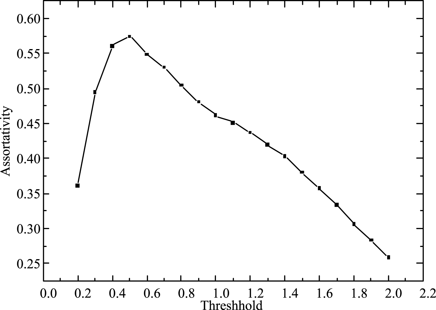
Relationship between threshold and assortativity.

Then, the relationship between the threshold and network entropy is studied. As shown in Fig. 2, the network entropy increases rapidly first and then increases slowly with the increase of the threshold. The network entropy rises slowly after the threshold increases to 0.5.

Fig.2

Relationship between threshold and network entropy.

However, the relationship between isolation rate and the threshold is different. The isolation decreases rapidly and goes down to 0. It indicates that the threshold can’t be too large or the recurrence network can’t reveal the nonlinear nature of the time series. This has been shown in Fig. 3.

Fig.3

Relationship between threshold and isolation rate.

On the other hand, the global recurrence rate monotonically increases when the threshold increases, as shown in Fig. 4. It increases faster when the threshold values is greater than 0.5. Other characteristics (mean degree centrality, global clustering coefficient and transitivity) of the recurrence network have similar relationships.

Fig.4

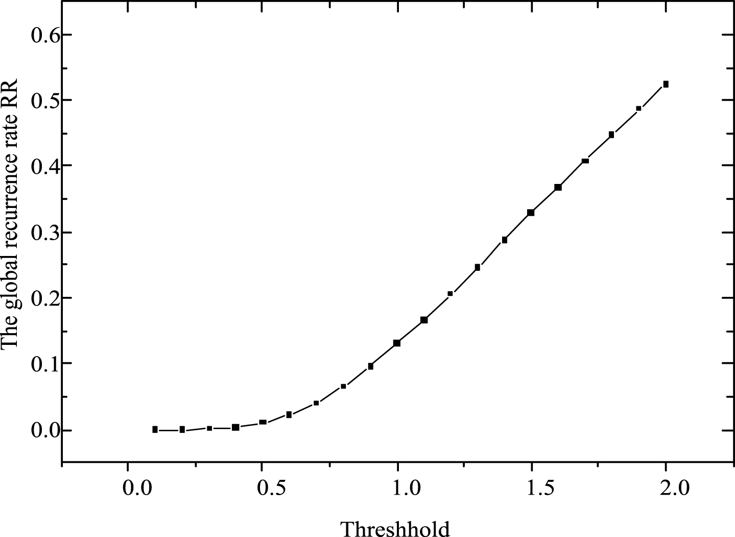
Relation between threshold and global recurrence rate.

From the above study, 0.5 is chosen as the threshold value, which guarantees the continuity of the density of states.

Besides, the false nearest neighbors (FNN) algorithm is used to determine the embedding dimension for the vibrational time series [16], and mutual information is used to determine the time delay [11].

3 Classifiers

3.1 Support vector machines

The basic idea of a binary SVM is to project data from the training data set to a high dimensional space and find an optimal hyper-plane, which separates the data with the maximal margin [5].

Given a data set $D_{Training} = {(x_{i}, y_{i})}_{i = 1}^{L}$ , where x_i ∈ Rⁿ is the input, and y_i∈ { - 1, + 1 } is the corresponding output, the input can be mapped into a high dimensional feature space F via a non-linear function Φ (x) : Rⁿ → F, by z = Φ (x). As a result, the input data can be linearly separated in F. This can be differentiated by a hyperplane, which is defined by a vector w ∈ F and a scalar b as $y_{i} (w^{'} \cdot z_{i} + b) \geq 1 - ξ_{i}, \forall i$ (16) where ξ_i ≥ 0 is slack variable. The optimal hyperplane should minimize $\frac{1}{2} \cdot w^{'} \cdot w + C_{w}$ (17) subject to $y_{i} (w^{'} \cdot z_{i} + b) \geq 1 - ξ_{i} \geq 0, \forall i$ (18) where C_w is the regularization parameter, which is used to balance the maximum margin and the minimum classification error. The above optimization problem can be solved by maximizing $w (α) = \sum_{i = 1}^{L} α_{i} - \frac{1}{2} \sum_{i = 1}^{L} \sum_{j = 1}^{L} α_{i} α_{j} y_{i} y_{j} k (x_{i}, x_{j})$ (19) subject to $\sum_{i = 1}^{L} y_{i} α_{i} = 0, 0 \leq α_{i} \leq C_{w}, \forall i$ (20) where α₁, …… , α_L represent non-negative Lagrangian multipliers. The data point x_i that satisfies the condition α_i > 0 is called support vector (SV). Correspondingly, the weight vector w can be expressed as $w = \sum_{SVs} α_{i} y_{i} z_{i}$ (21)

Given a test vector x_t ∈ Rⁿ, the classification output can be obtained as $y_{t} = sign (w \cdot z + b) = sign (\sum_{SVs} α_{i} y_{i} K (x_{i}, x) + b)$ (22)

SVM is a non-linear classifier based on kernel function [8]. Typically, the radial basis function is used as the kernel function, which is expressed as $K (x_{i}, x) = exp (- \frac{{∥ x_{i} - x ∥}^{2}}{2 σ^{2}})$ (23) where σ is a width parameter which determines the range of the kernel function.

In order to transform the binary SVM into multi-class SVM, the one-against-one (OAO) strategy is adopted [13].

3.2 Extreme learning machine

ELM is a new learning algorithm for a single-hidden-layer feedforward network (SLFN) [18]. Parameters of the hidden-layer node are obtained by mathematical calculation rather than iterative adjustment in ELM, which shows good generalization performance with higher speed than traditional learning algorithms for feedforward neural networks [15]. In a SLFN with M hidden nodes, the output f_M (x_j) can be represented by $f_{M} (x_{j}) = \sum_{i = 1}^{M} β_{i} g (w_{i} x_{j} + b_{i}), x_{j} \in R^{n}$ (24) where w_i and b_i are the weight vector and the bias between the input and the ith hidden node, and β_i is the weight of the ith hidden node connected to the output node. g (•) is the activation function, and the sigmoidal function $g (x) = \frac{1}{1 + e^{- λ x}}$ is used as activation function in this study for ELM.

If a SLFN with M hidden nodes can realize zero error to approximate N samples (x_j, t_j) ∈ Rⁿ × R^m, j = 1, 2, … N, where x_j is an n-dimensional input vector and t_j is an m-dimensional target vector, it means Equation (24) can be rewritten as: $\sum_{i = 1}^{M} β_{i} g (w_{i} x_{j} + b_{i}) = t_{j}, j = 1, 2, \dots, N$ (25)

Equation (25) can be rewritten as $H β = T$ (26) where $\begin{matrix} H (w_{i}, b_{i}, x_{j}) \\ = [\begin{matrix} g (w_{1}, b_{1}, x_{1}) & \dots & g (w_{M}, b_{M}, x_{1}) \\ ⋮ & ⋱ & ⋮ \\ G (w_{1}, b_{1}, x_{N}) & \dots & g (w_{M}, b_{M}, x_{N}) \end{matrix}] \\ β = {[\begin{matrix} β_{1}^{T} \\ ⋮ \\ β_{M}^{T} \end{matrix}]}_{M \times m} and T = {[\begin{matrix} t_{1}^{T} \\ ⋮ \\ t_{N}^{T} \end{matrix}]}_{N \times m} \end{matrix}$

H is the hidden layer’s output matrix of the network [15]; H’s ith column is the ith hidden node’s output vector corresponding to inputs x₁, x₂, …, x_N and H’s jth row is the output vector of the hidden layer with respect to input x_j.

The parameters of the hidden node, w_i and b_i in the SLFNs don’t need to be adjusted during training. The parameters may simply be allocated with random values based on any continuous sampling distribution. This makes Equation (26) a linear system, and the output weights are estimated as $\tilde{β} = H^{†} T$ (27) where H^† is the generalized inverse of the hidden layer output matrix H [15].

Huang et al. [14] have proved the universal approximation ability of ELM via an incremental method.

4 Experimental evaluation

To utilize the quantitative measures obtained from the recurrence network for characterizing the gear states, Fig. 5 shows the flowchart of recurrence network-based fault diagnosis approach. The time series of vibrational signals measured by sensors are transformed into phase space using embedding theory. Then the vectors in phase space are transformed into the recurrence network by maximum norm associated with a suitable threshold. After that, quantitative measures are calculated from the recurrence network, and used as the input to the classifiers for gear fault diagnosis.

Fig.5

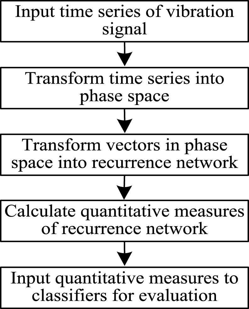
The flowchart of the proposed method.

4.1 Fault severity evaluation

The first experimental study was conducted on a four-speed motorcycle gearbox test system [22]. As shown in Fig. 6, the electrical motor was run at a constant speed at 1420 RPM. In order to eliminate the vibration, four shock absorbers were installed under the base of the test system. Four different fault conditions were tested in this study, which include slight-worn gear, medium-worn gear, broken teeth of gear and one normal condition, respectively.

Fig.6

Experimental setup of motorcycle gearbox test system.

Signals were sampled at 16384 Hz, and the raw vibration signals of four conditions are shown in Fig. 7. The embedding dimension and time delay is set as 6 and 2, respectively.

Fig.7

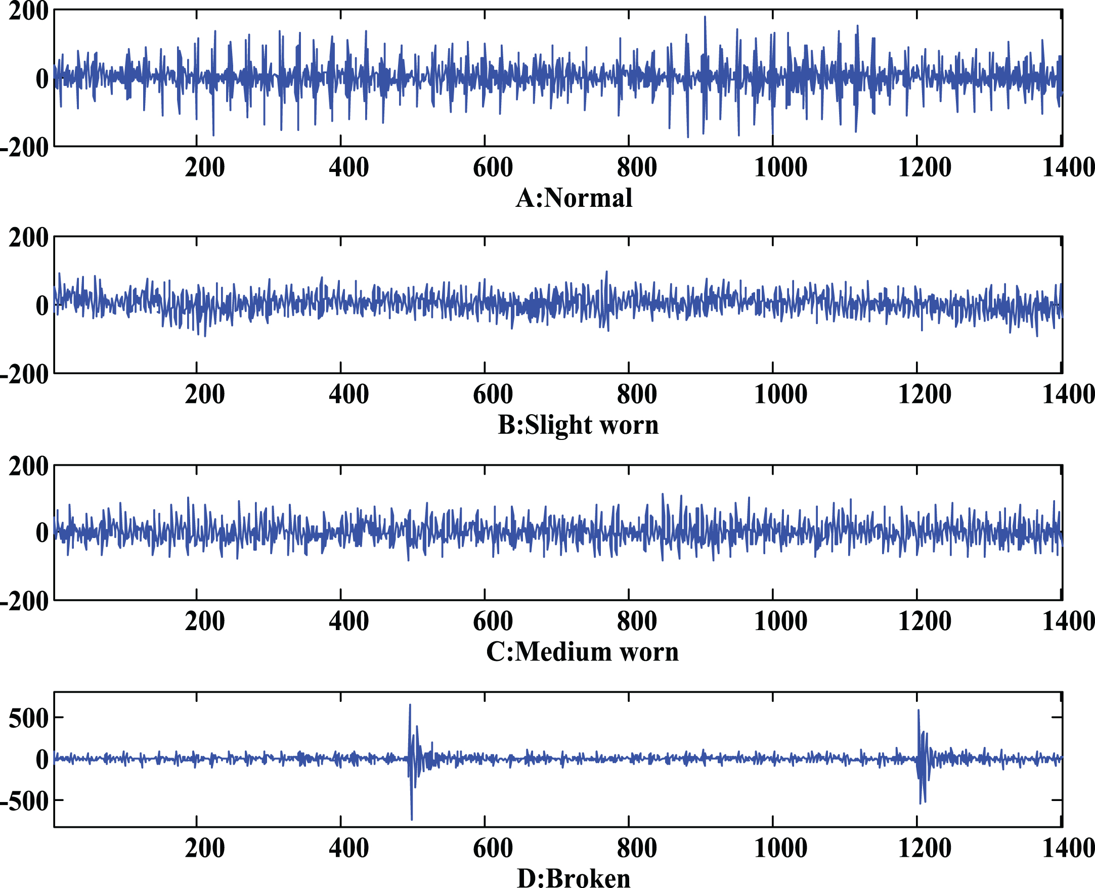
Vibration signals measured on motorcycle gearbox.

The conditions of the gear can’t be recognized directly from the waveforms of the vibration signals. Through recurrence network theory, different features of the vibration signals are obtained. In this paper, the mean degree of all vertices <k>, global edge density ρ, the global clustering coefficient C, assortativity A_s, network transitivity T, network entropy H_SE and isolation rate IR are used as the features of the vibration signals. Forty sets of data are chosen for each gear type. Table 2 lists sample features extracted four different conditions.

Table 2

Features extracted from different motorcycle gearbox conditions

Faults	Normal	Slight worn	Medium worn	Tooth broken
<k>	15.291	2.4953	2.961	18.614
ρ	0.011	0.001	0.002	0.013
C	0.290	0.159	0.153	0.297
A_s	0.586	0.342	0.505	0.564
T	0.339	0.208	0.213	0.347
H_SE	6.611	6.755	6.689	6.565
IR	0.103	0.234	0.236	0.125

To classify the conditions of the gear, ELM and SVM are used as the classifiers. 80 data samples with each condition containing 20 samples are used to train the classifiers, and another 80 data samples are used for testing. < k>, ρ, C, A_s, T, H_SE and IR are used as the features to the input of the classifiers. From Tables 3 and 4, 13 data samples are misclassified using SVM and the classification accuracy is 83.75%, while only four data samples are wrongly classified using ELM, and the classification accuracy is 95%. The comparison shows that ELM has better performance than SVM. The result also indicates quantitative measures extracted from recurrence network can characterize the gear severity effectively.

Table 3

Results for four different gear conditions using SVM

Faults	Normal	Slight worn	Medium worn	Tooth broken
Normal	17	0	0	3
Slight worn	0	18	2	0
Medium worn	0	3	17	0
Tooth broken	5	0	0	15

Table 4

Results for four different gear conditions using ELM

Faults	Normal	Slight worn	Medium worn	Tooth broken
Normal	20	0	0	0
Slight worn	0	20	0	0
Medium worn	0	1	19	0
Tooth broken	3	0	0	17

To further illustrate the effectiveness of the presented approach, some statistical parameters, including root mean square, peak, kurtosis, deviation coefficient, pulse and margin, were also extracted as input to ELM classifier for gear fault diagnoisis. The mathmatical expressions of these parameters are listed in Table 5, where x(t) represents the original gear vibration signal, μ is the average value of the signal x(t) and x_p is the peak value of the signal. The diagnostic results are shown in Table 6, where 7 data samples are misclassified, leading to 91.25% classification accuracy, which is lower than that of reccurrence network-based approach.

Table 5

Time-domain statistical features used in this study

Features	Mathematical expression
Root mean square	$X_{rms} = \sqrt{\frac{1}{N} \sum_{t = 1}^{N} x (t)^{2}}$
Peak index	$P_{k} = \frac{x_{p}}{X_{rms}}$
Kurtosis	$K_{ur} = \frac{1}{N} \sum_{t = 1}^{N} {(\frac{x (t) - μ}{σ})}^{4}$
Deviation coefficient	$S_{f} = \frac{X_{rms}}{\frac{1}{N} \sum_{t = 1}^{N} \| x (t) \|}$
Pulse index	$I_{p} = \frac{x_{p}}{\frac{1}{N} \sum_{t = 1}^{N} \| x (t) \|}$
Margin index	$M_{I} = \frac{x_{p}}{\| \frac{1}{N} \sum_{t = 1}^{N} \sqrt{\| x (t) \|} \|}$

Table 6

Features from time domain using ELM

Faults	Normal	Slight worn	Medium worn	Tooth broken
Normal	15	0	5	0
Slight worn	2	18	0	0
Medium worn	0	0	20	0
Tooth broken	0	0	0	20

4.2 Gear fault classification

The second experimental study was conducted on a Drivetrain Dynamics Simulator (DDS) platform for characterizing different types of gear faults, as shown in Fig. 8. Table 7 lists different gear faults tested in this study. Vibration signals are acquired with 1024 Hz sampling rate and 512 s sampling window when the simulator is running at 30 Hz rotating speed.

Fig.8

Experimental setup of a DDS system.

Table 7

Different types gear faults in DDS system

Faults	Miss	Chipped	Surface
Description	One of tooth is missing.	A crack occurs in one tooth.	The wear occurs in the surface.
Product

Figure 9 illustrates the waveforms of the gearbox vibration signals under four different working conditions. Using the FNN algorithm and mutual information, the embedding dimension and time delay are selected as 6 and 2, respectively. Threshold for constructing recurrence matrix is set as 0.4. Through recurrence network theory, the features < k>, ρ, C, A_s, T, H_SE and IR are also extracted from the vibration signals, and Table 8 lists sample features from each condition.

Fig.9

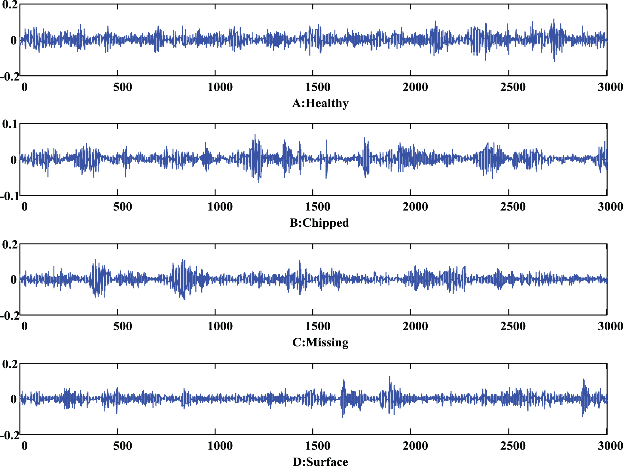
Raw vibration signals of four gearbox conditions.

Table 8

Features extracted for different types of gear faults

Fault	Healthy	Chipped	Missing	Surface
<k>	4.908	26.799	11.571	3.738
ρ	0.002	0.009	0.004	0.001
C	0.122	0.204	0.159	0.113
A_s	0.631	0.489	0.556	0.652
T	0.255	0.353	0.309	0.266
H_SE	6.963	6.997	6.887	6.862
IR	0.388	0.311	0.367	0.461

To classify different gearbox conditions, 160 data samples are used to train the classifiers with each condition including 40 data samples. The same numbers of data samples in each condition are used for testing. From Tables 9 and 10, fifteen data are misclassified when SVM is used as the classifier, leading to 87.5% classification accuracy, while nine data are wrongly classified when ELM is used as the classifier, which corresponds to 92.5% classification accuracy. Again comparison study shows that ELM has better performance than SVM. Features extracted based on recurrence network can effectively characterize the gear working conditions.

Table 9

Results for different types of gear faults using SVM

Faults	Healthy	Chipped	Missing	Surface
Healthy	32	0	0	8
Chipped	0	40	0	0
Missing	1	0	39	0
Surface	6	0	0	34

Table 10

Results for different types of gear faults using ELM

Faults	Normal	Chipped	Missing	Surface
Healthy	38	0	0	2
Chipped	0	40	0	0
Missing	0	0	40	0
Surface	7	0	0	33

The statistical paramters presented in the first experimental study are also calculated here and used as input to the ELM classifier. As listed in Table 11, 15 data samples are misclassified, leading to 87. 5%, classification accucry, which is 5 percent less than that of recurrence network features. This again proves the effectiveness of the presented approach for gear fault diagnosis.

Table 11

Features from time domain using ELM

Faults	Normal	Chipped	Missing	Surface
Healthy	39	0	1	0
Chipped	0	34	6	0
Missing	3	2	35	0
Surface	1	0	2	37

5 Conclusion

A recurrence network-based approach is introduced in this paper for gear fault diagnosis, in which various quantitative measures, such as the mean value of all vertices, global recurrence rate, the global clustering coefficient, assortativity, network transitivity, and isolation rate, are extracted as features to characterize the vibration signals. Two experimental case studies are investigated to verify the effectiveness of recurrence network as a means for characterizing gear working conditions. The results show that recurrence network can not only evaluate gear fault severity, but also classify different gear faults. In summary, recurrence network provides a good and powerful mathematical tool for nonlinear time series analysis with great potential to machine fault diagnosis.

Footnotes

Acknowledgments

This work has been supported by the National Natural Science Foundation of China (51575102), Six talent peaks project in Jiangsu Province (JXQC-003), and Fundamental Research Funds for the Central Universities of China(2242017K40112).

References

Aherwar

, Khalid

, Vibration analysis techniques for gearbox diagnostic: A review, Int J Adv Eng Technol E1 (3) (2012), 101–113.

Barrat

, Weigt

, On the properties of small-world network models, Eur Phys J B13 (2000), 547–560.

Barszcz

, Jabłoński

, A novel method for the optimal band selection for vibration signal demodulation and comparison withthe Kurtogram, Mechanical Systems & Signal Processing25, (1) (2011), 431–451.

Boccaletti

, Latora

, Moreno

, Chavez

, Hwang

D.U.

, Complex networks: Structure and dynamics, Phys Rep424 (4-5) (2006), 175–308.

Cherkassky

, The nature of statistical learning theory, IEEE Transactions on Neural Networks8, (6) (1997), 1564.

Crucitti

, Latora

, Marchiori

, A topological analysis ofthe Italian electric power grid, Physica A Statistical Mechanics & Its Applications338 (1) (2004), 92–97.

Davidsen

, Grassberger

, Paczuski

, Networks of recurrent events, a theory of records, and an application to finding causal signatures in seismicity, Physical Review E Statistical Nonlinear & Soft Matter Physics77 (6 Pt 2) (2008), 066104.

Ding

, Chen

, Classification of hyperspectral remote sensing images with support vector machines and particle swarm optimization, International Conference on Information Engineering and Computer Science. IEEE, (2009), 1–5.

Diwakar

, Satyanarayana

M.R.S.

, Kumar

P.R.

, , Detection of gear fault using vibration analysis, 2014.

10.

Donner

R.V.

, Zou

, Donges

J.F.

, . Recurrence networks - Anovel paradigm for nonlinear time series analysis, New Journal of Physics12 (3) (2009), 129–132.

11.

Fraser

A.M.

, Swinney

H.L.

, Independent coordinates for strange attractors from mutual information, Physical Review A General Physics33 (2) (1986), 1134–1140.

12.

Gao

, Jin

, Flow-pattern identification and nonlinear dynamics of gas-liquid two-phase flow in complex networks, Phys Rev E Stat Nonlin Soft Matter Phys79 (2) (2009), 066303.

13.

Hsu

C.W.

, Lin

C.J.

, A comparison of methods for multiclass support vector machines, IEEE Transactions on Neural Networks13 (4) (2002), 1026.

14.

Huang

G.B.

, Chen

, Siew

C.K.

, Universal approximation using incremental constructive feedforward networks with random hidden nodes, IEEE Transactions on Neural Networks17 (4) (2006), 879–892.

15.

Huang

G.B.

, Zhou

, Ding

, . Extreme learning machine for regression and multiclass classification, IEEE Transactions on Systems Man & Cybernetics Part B42 (2) (2012), 513–529.

16.

Kennel

M.B.

, Brown

, Abarbanel

H.D.

, Determining embedding dimension for phase-space reconstruction using a geometrical construction, Physical Review A Atomic Molecular & Optical Physics45 (6) (1992), 3403.

17.

, Costa

, Rodrigues

F.A.

, Travieso

, . Characterization of complex networks: A survey of measurements, Advances in Physics56 (1) (2007), 167–242.

18.

Lan

, Soh

Y.C.

, Huang

G.B.

, Extreme learning machine based bacterial protein subcellular localization prediction, IEEE International Joint Conference on Neural Networks. IEEE, 2008, 1859–1863.

19.

Marwan

, Romano

M.C.

, Thiel

, Recurrence plots for the analysis of complex systems, Physics Reports438 (5) (2007), 237–329.

20.

Nacib

, Saad

, Sakhara

, A Comparative study of various methods of gear faults diagnosis, Journal of Failure Analysis and Prevention14 (5) (2014), 645–656.

21.

Newman

M.E.

, Assortative mixing in networks, Physical Review Letters89 (20) (2002), 208701.

22.

Rafiee

, Tse

P.W.

, Use of autocorrelation of wavelet coefficients for fault diagnosis, Mechanical Systems & Signal Processing23 (5) (2009), 1554–1572.

23.

Ramírez Ávila

G.M.

, Gapelyuk

, Marwan

, , Classification of cardiovascular time series based on different coupling structures using recurrence networks analysis, Philosophical Transactions of the Royal Society A Mathematical Physical & Engineering Sciences3712013, 20110623.

24.

Saravanan

, Cholairajan

, Ramachandran

K.I.

, Vibration-based fault diagnosis of spur bevel gear box using fuzzy technique, Expert Systems with Applications An International Journal36 (2) (2009), 3119–3135.

25.

Saravanan

, Ramachandran

K.I.

, Fault diagnosis of spur bevel gear box using discrete wavelet features and Decision Tree classification, Expert Systems with Applications36 (5) (2009), 9564–9573.

26.

Schinkel

, Dimigen

, Marwan

, Selection of recurrence threshold for signal detection, The European Physical Journal Special Topics164 (1) (2008), 15–53.

27.

Small

, Zhang

, Xu

, Transforming Time Series into Complex Networks. Complex Sciences. SpringerBerlin Heidelberg, (2009), 2078–2089.

28.

Subramaniyam

N.P.

, Hyttinen

, Characterization of dynamical systems under noise using recurrence networks: Application to simulated and EEG data, Physics Letters A378 (46) (2014), 3464–3474.

29.

Sun

, Liang

, Shang

, Rolling bearings fault diagnosis based on recurrence complex network, Journal of Vibration Measurement & Diagnosis35 (3) (2015)578–584.

30.

Bin

, Da

, Complex network in application of rotor faultdiagnosis, Journal of Vibration, Measurement & Diagnosis32 (6) (2012), 1010–1015.

31.

Takens

, Detecting strange attractors in turbulence, in dynamical systems and turbulence, warwick, Lecture Notes in Mathematics898 (1981).

32.

, Tan

Y.J.

, Deng

H.Z.

, . A new measure of heterogeneity of complex networks based on degree sequence, 2010, 66–73.

33.

Zhou

, Zemanová

, Zamora

, . Hierarchical organization unveiled by functional connectivity in complex brain networks, Physical Review Letters97 (23) (2006), 238103.

Gear fault diagnosis based on recurrence network

Abstract

Keywords

1 Introduction

2 Theoretical background

2.1 Transforming time series into phase space

Table 1 Relationship between recurrence network and phase space Recurrence Network Phase Space Vertex State xt Edge Recurrence of states Path Overlapping sequence of ɛ-balls

3.1 Support vector machines

Footnotes

Acknowledgments

References

Table 1
Relationship between recurrence network and phase space

Recurrence Network Phase Space

Vertex State x_t

Edge Recurrence of states

Path Overlapping sequence of ɛ-balls