
Abstract
The prediction of performance degradation is significant for the health monitoring of rolling bearing, which helps to greatly reduce the loss caused by potential faults in the entire life cycle of rotating machinery. As a new method of machine learning based on statistical learning theory, a so-called multivariable least squares support vector machines (LS-SVM) was developed. However, it is unsatisfactory for the prediction of performance degradation without adequate consideration of time variation and data volatility, which are notable features of the obtained time series signal from bearings. To overcome these problems, a new multivariable LS-SVM with a moving window over time slices is proposed. In this model, different features over time slices are extracted through a moving window to construct new sample pairs according to the embedding theory. The model adaptability is also improved through an iterative updating strategy. Furthermore, the algorithm parameters are optimized using coupled simulated annealing to improve the prediction accuracy. Bearing fault experiments show that the proposed model outperforms the general multivariable LS-SVM.
Keywords
Introduction
Rotating machinery plays an important role in modern industry, and gradually tends to be high-performing, large-scale and complex. As one of the key components in rotating machinery, rolling bearings are easily damaged, and the bearing failure may result in significant loss in production and human casualties [1]. To ensure the safety of the machinery, prognostics and health management (PHM), including the prediction of performance degradation, has attracted much attention. PHM can be used to conduct timely maintenance, provide spare parts supplies and intelligent accident prevention [2, 3].
Recently, technologies related to equipment condition monitoring provide a good basis for the degradation trend prediction of rolling bearings. It is feasible to improve the accuracy of the prediction by collecting vibration signals and mining appropriate information from the time, frequency and time-frequency domains [4]. Data-driven approach is one of the most common methods for degradation trend prediction. These methods usually construct prediction models from historical data, using pattern recognition or machine learning techniques to predict future values, such as the Wiener process [5] and stochastic filtering-based models [6]. The effectiveness of the statistical learning methods often depends on the amount of data.
However, bearing failure or performance degradation occurs at a small probability, compared to that of a healthy-operating status in most time. Therefore, compared to the large healthy datasets, it is difficult to collect enough data related to the performance degradation. It is necessary to find new ways to solve these problems using limited data samples of bearing degradation. Support vector machines (SVM) or the improved least squares SVM (LS-SVM) provides a suitable way to solve small sample problems [7, 8]. Recently, LS-SVM made great progress in many fields such as pattern recognition with high dimension [9] and function regression [10]. It can be used to avoid the dimensionality curse and has great advantages in nonlinear time series prediction [11]. Therefore, it provides an important inspiration for the degradation trend prediction of rolling bearing.
Most traditional trend prediction methods, including LS-SVM, often make predictions using a single variable model [12, 13], i.e., predicting the dependent variable values as a function of an independent variable. However, the degradation performance is affected by multiple factors. A so-called multivariable LS-SVM is then proposed, which aims to determine the relationship between the predictor y and multiple variables x1 (i) , x2 (i) , …, x m (i). This helps to explore more internal information about y from multiple variables [14].
The general multivariable LS-SVM has been widely used in degradation trend prediction and achieved remarkable results. However, similar biological studies have shown that the output of synapses in biological neurons depends on the input process that continues for a certain period of time. The training sample and prognosis sample in the general multivariable LS-SVM lacks consideration of the data influence over time, and also ignores the impact of data fluctuations on the prediction accuracy.
A bearing vibration signal is a typical temporal sequence. If a fault occurs in a rolling bearing, the indicative features obtained from the collected vibration signals are often monotonically changing. Based on this changing relationship, it is helpful to improve the adaptability of the prediction model. According to the embedding theory [15], there usually exists a functional relationship between the future value and the previous values in a temporal sequence, i.e., contextual relationship. Because the general LS-SVM lacks consideration of the contextual influences of the temporal signal, it does not work well for estimating the evolution of bearing performance degradation.
To solve these problems, we proposed a multivariable LS-SVM over time slices, according to the embedding theory. In the proposed model, different characteristics at different time moments are employed in the construction of training and test samples. In addition, both the influence of data volatility and contextual influences are fully considered. First, different features are extracted from the denoised signal, which aims to remove the interference of the environment. Next, correlation analysis is used to select the appropriate sensitive features, which aims to improve the prediction accuracy. Finally, the chosen features at different time moments are used to train the model.
Moreover, the general LS-SVM often requires a fixed number of training samples. However, actual vibration signals of rolling bearing are often nonstationary, which has a significant impact on the prediction accuracy. With the bearing performance gradually degrading, the signal features will change significantly. The prediction model with the general LS-SVM is unsuitable for this kind of signal, which may lead to a decrease in prediction accuracy. Therefore, we employ a moving window to update the model training process. We update the trained model by adding new samples to the training set and discarding earlier samples. The addition of new samples makes the model adaptive and dynamic. Due to the removal of the earlier samples, the computational complexity of the model is not increased significantly.
The main contribution of this work can be summarized as follows. First, we developed a prediction model for the bearing performance degradation based on the multivariable LS-SVM and embedding theory, which accounts for the data volatility and contextual influences. Second, to better describe the dynamic feature changes of the signal sequence, a model update method is employed with a moving window over time slices.
The remainder of the paper is organized as follows. The general multivariable LS-SVM prediction model is briefly introduced in Section 2. The multivariable LS-SVM over time slices is presented in Section 3. Experiments are conducted using the proposed method in Section 4 and the conclusion is presented in Section 5.
General multivariable LS-SVM model
LS-SVM is the least squares version of support vector machine. The insensitive loss function in SVM is replaced by a mean error cost function [16]. Therefore, the inequality constraints are replaced by equality constraints and the quadratic programming problem is converted into the linear equation problem. Therefore, the computational complexity of LS-SVM is smaller than that of SVM because of this reformulation.
For a group of given training samples
In order to solve the optimization problem in Equation (2), the Lagrangian function is introduced to solve the dual problem, and the optimization problem is transformed into the convex quadratic programming problem, which can be solved by the Lagrange multiplier. The Lagrangian function is
By solving Equation (5), the final regression function can be obtained as
According to the embedding theory, for a set of time series, there is a functional relationship between the future value of the sequence and the previous values. The expression is
Therefore, if the first n samples are used to train the model, the training sample pair and prognosis sample input can be constructed as [17]
The actual development of the rolling bearing failure is often affected by many factors. The single variable LS-SVM has a simple structure, and cannot represent information contained in other variables. In addition, it only uses the implicit dependencies between the data of the series for the next step. Therefore, it cannot fully reflect the degradation trend performance. The multivariable LS-SVM considers the interaction between multiple variables and their coordinated development, which can achieve a maximum mining of potential information from a signal. The multivariable LS-SVM makes use of different features to predict the future value of the sequence. It tries to determine the relationship between the value y1 and the multiple variables x1 (i) , x2 (i) , …, x
m
(i) by constructing the following prediction model
The training sample pair and prognosis sample input of the multivariable LS-SVM can be reformulated as Equations (12–14).
The predictive results of the single variable LS-SVM are susceptible to randomness of the history data sequence, which may affect the prediction accuracy. However, the multivariable LS-SVM eliminates a variety of adverse effects by accounting for the interaction of multiple variables and constraints, which will result in more accurate predictions.
In order to exploit more information about the vibration signals, improve the prediction accuracy and make the prediction model adaptable to the monitoring signal, a kind of moving window multivariable LS-SVM over time slices is proposed, as shown in Fig. 1.
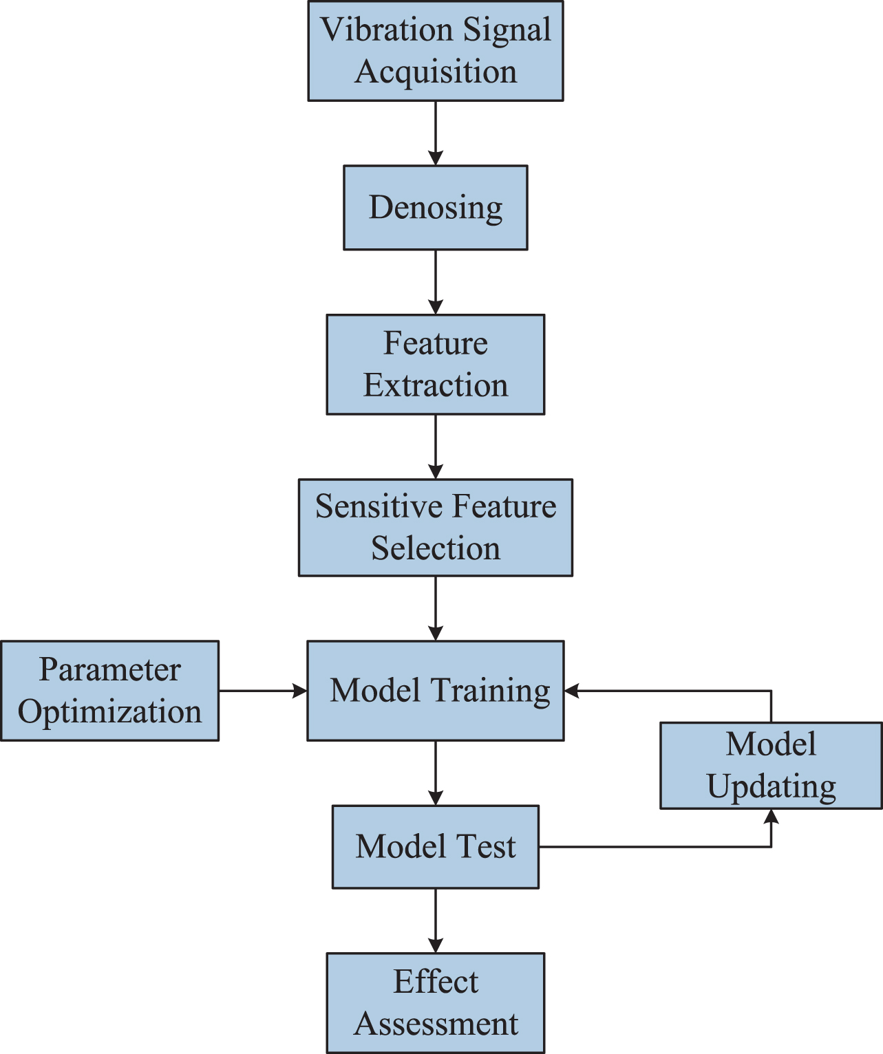
Flowchart of the proposed method.
The proposed multivariable LS-SVM over time slices not only considers the mutual influence of multi-variables, but also takes into account the impact of the signal volatility. As the embedding theory shows in Equation (7), the future value of the sequence is related to previous values. Therefore, based on the multivariable LS-SVM introduced in Section 2, a new sample structure is constructed as Equations (15 and 16).
The subscript i in (15) represents the number of variables. For each variable, there are m values used for prediction. The schematic diagram of the construction method is shown in Fig. 2.

Schematic diagram of the construction method.
The proposed structure of the sample pair makes great use of data information, and improves the prediction accuracy. The main steps of the proposed method are: Signal acquisition and preprocessing: Collect the vibration signals of rolling bearings. The signals are denoised by wavelet thresholding, aiming to remove environmental impact. Feature selection: To fully reflect the degradation trend performance, it is important to select appropriate features. Several features in the time, frequency and time-frequency domains are extracted. At the same time, correlation analysis is used to select the appropriate features to construct the training sample pairs. These features have similar trend characteristics, which may improve the performance of degradation trend prediction. Construct multivariable LS-SVM over time slices: Training samples are constructed according to Equations (20 and 21), using the sensitive features in Step 2 to obtain the final regression function in Equation (9). The proposed model is then used to predict the degradation performance with the prognosis sample. Prognosis effect assessment: Root mean square error e
RMSE
, mean absolute error e
MAE
and cross-correlation coefficient R2 are chosen to evaluate the proposed model, using the expression.
Among the above formulas, y
i
represents the actual data and
In the LS-SVM model introduced in Section 2, there are two parameters to be determined: the penalty coefficient and variance in the RBF kernel used in this paper. Simulated annealing (SA) provides a good way for doing this, which is based on the solid annealing process to obtain optimization parameters. It is a stochastic optimization algorithm based on a Monte-Carlo iterative solution. It accepts the parameters with low fitting accuracy, and avoids the algorithm falling into the local optimum. The main steps of the SA algorithm are: Initialization: Assign a random initial solution to x. Assess the cost E (x) and set the initial temperatures T
k
= T0 and Generate a probing solution y according to y = x + ɛ, where ɛ is acquired from a given distribution g (ɛ, T
k
). Next, assess the cost for the new solution. Accept the solution y with the probability 1 while E (y) < E (x). Otherwise, accept it with the probability A (x → y). Change the temperatures according to the generation temperature schedule U (T
k
, k) and acceptance temperature schedule Stop when the equilibrium criterion is met. The flowchart of the SA algorithm is shown in Fig. 3.
However, the convergence speed of the SA is slow, which is not conducive to online optimization. On the other hand, the robustness of the SA is affected by the initial assignment of temperature. In order to solve this problem, coupled simulated annealing (CSA) is used to optimize the parameters in this model. The CSA algorithm realizes the mutual coupling and information sharing of each SA process by the coupling terms, which reflect the energy and state of the accepted probability function [18]. The matching of the accepted function and the coupling term leads the CSA algorithm to the global optimal solution. The main difference between the SA and CSA algorithm lies in the acceptance process, as shown in Fig. 4.
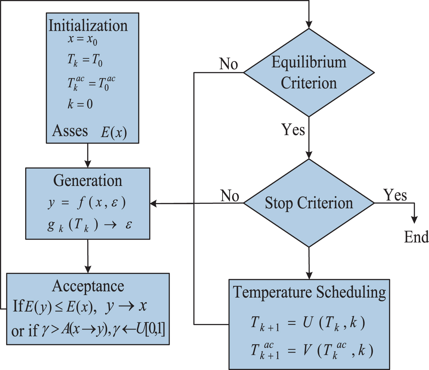
Flowchart of the SA algorithm.

The main differences between SA and CSA algorithm [18].
To construct the proposed LS-SVM model, there are two parameters (super parameters) to be determined: the penalty coefficient and kernel parameter. According to the CSA algorithm, there are super parameter generation and acceptance processes. The generation process is:
Therefore, the CSA algorithm accepts the super-parameter with high fitting performance, and accepts the super-parameter with poor accuracy with a certain probability. This promotes the sharing of information in the independent SA algorithm optimization.
According to the prediction model, the prediction performance relies on the correlation between the training signals and the test signals. However, actual vibration signals of rolling bearing are nonlinear. Therefore, the offline training method is not suitable for the trend prediction of nonlinear signals. In the signal acquisition process, more new samples will be acquired. To better track the dynamic changes of the signal, the prediction model is updated with a moving window.
In the moving window model, the trained LS-SVM is updated by incrementing the training set with new samples and discarding the oldest sample in the training set [19]. In this case, the development of the LS-SVM allows the model to more effectively track the nonstationary dynamics in the vibration signal of bearing. What is more, the number of data pairs used to train the model remains constant by removing the oldest data pairs, thereby reducing the computational complexity. There are two main algorithms in the moving window LS-SVM: incremental and decremental algorithms. The incremental algorithm updates the trained LS-SVM (of N data pairs) by adding a new training sample (N + 1 data pair). Therefore, the latest data is used in the model construction. Meanwhile, in order to not increase the computational complexity, the decremental algorithm removes the beginning sample pairs from the training pairs, whose contribution to the model is negligible, and maintains a constant number of data pairs.
The main steps of the moving window multivariable LS-SVM are as follow: Initialization: Initialize the training sample pairs according to Equations (15) and (16). Next, use the CSA algorithm to acquire the initial LS-SVM model. Update training sample pair: The incremental algorithm is employed to increment the training sample pair, and the decremental algorithm is employed to discard the oldest training pair. Prediction: According to the new training sample pairs constructed from step 2, a new proposed multivariable LS-SVM model is trained to predict the future value. Repeat Steps 2-3 until the end of the degradation trend prediction. Above all, the update process is shown as Fig. 5.
Experiment
To verify the effectiveness of the proposed method, we verified the proposed method with the entire life data of the rolling bearing from healthy status to failure [20]. The performance is compared with that from the general multivariable LS-SVM. The test rig is shown in Fig. 6. There are two accelerometers placed radially on the external race of the bearing in vertical and horizontal directions. The load is applied radially to the bearing in the horizontal direction.
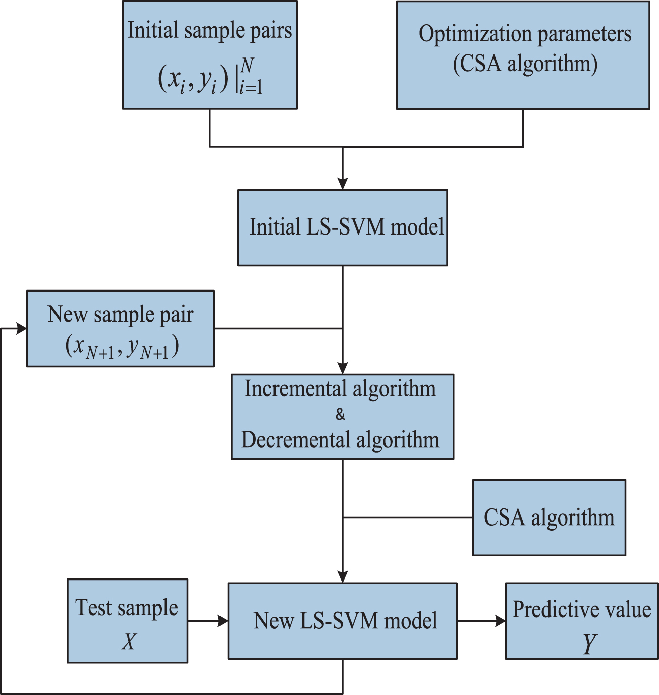
The model update of the LS-SVM algorithm.
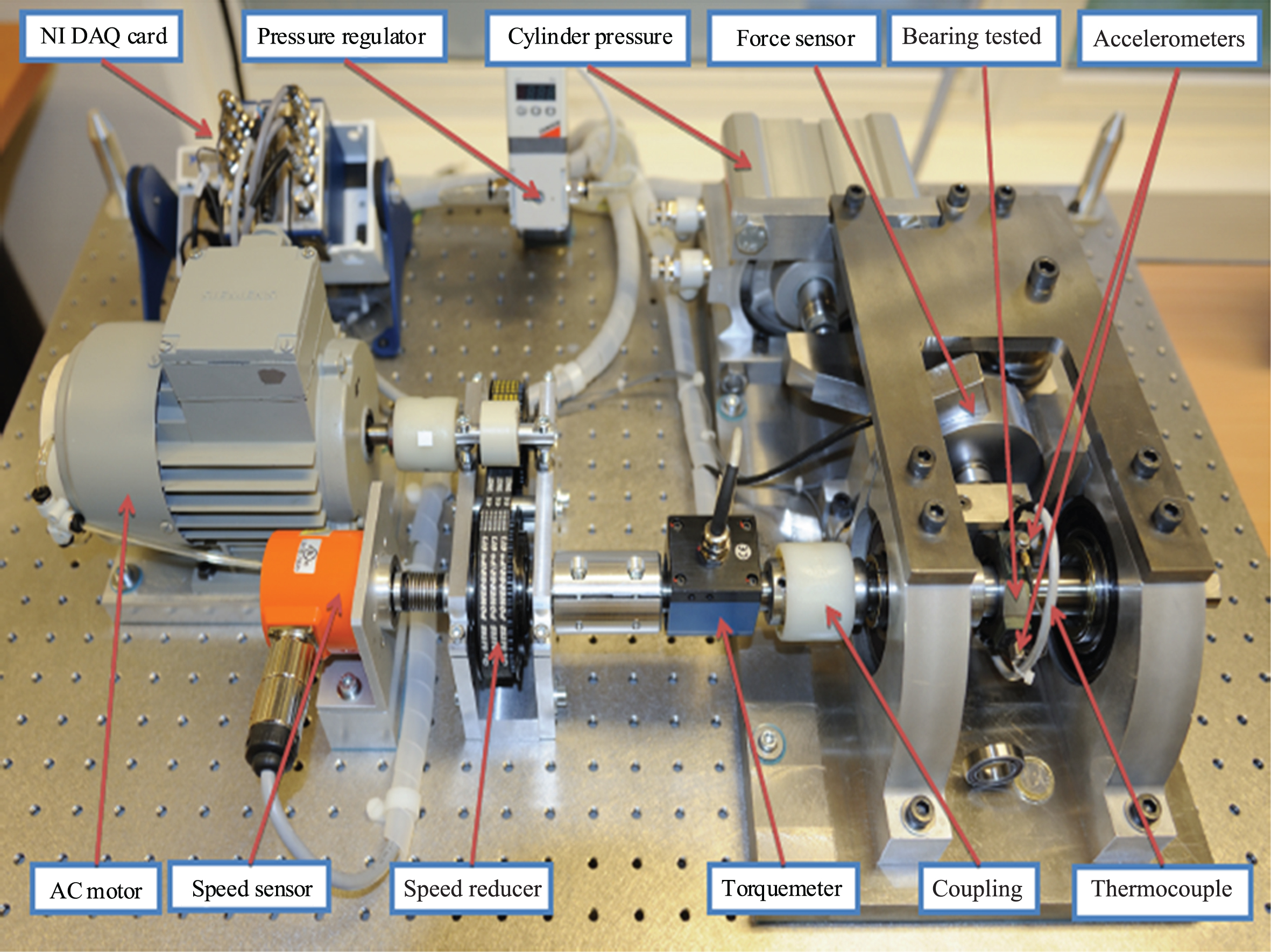
The test rig.
In this experiment, the vibration signal is recorded at a sampling frequency of 25.6 kHz every 10 s. A total of 1802 sets of data were recorded, each of which recorded 2506 points.
In order to reflect the state of rolling bearings well, the vibration signal is first denoised by wavelet thresholding to remove the influence of environmental noise. Next, the sensitive features in the time, frequency and time-frequency domains are extracted from the vibration signal, such as root mean square (RMS), mean (M), variance (VAR), spectral energy (E), and wavelet energy. The RMS value is extracted as the main feature to be predicted. The RMS of the life test is shown in Fig. 7.

RMS of the test.
According to Fig. 7, the RMS in the first 1200 data set was stable and there was no great volatility. Therefore, it can be judged that the bearing in the first 1200 minutes was in a normal state. However, the RMS gradually increased after the 1200th data set. It can be discerned that it was in a degradation state. In this experiment, the RMS between the 1400th and 1700th data set was utilized to train and validate the proposed model.
To select the appropriate sensitive features, the signal between the 1400th and 1700th data set is intercepted to extract kurtosis, mean, variance, energy spectrum and the energy of the first three layers after wavelet decomposition. In order to improve the performance of the prediction, correlation analysis is used as an effective way to determine interdependencies between variables. It chooses those features that are similar to the RMS. The main steps of the correlation analysis are: Extract features from vibration signals of the rolling bearing. Based on the RMS, the correlation between each relative feature and RMS is calculated by correlation analysis. Preset a threshold. When the correlation coefficient is greater than the threshold, the feature is retained. Otherwise it is removed.
The closer the correlation coefficient is to 1, the higher the correlation between the two variables. While the absolute value of the correlation coefficient is greater than 0.8, the two variables are highly correlated. Therefore, the threshold is set as 0.8 to choose the sensitive features that are similar to the RMS trend. According to the correlation coefficients in Table 1, there are three features selected: variance, mean, and energy spectrum.
The correlation coefficients
In order to scale the data, the various features need to first be normalized. In this experiment, the 1400th to the 1700th data set of the RMS, Var, M, and E are utilized to train and validate the proposed model. For the RMS, the first 280 sets of data are used as training samples, and the latter 20 sets are used as prediction samples. These chosen sensitive features are used to construct X train in Equation (7), where the parameter m is equal to 5. The corresponding RMS is used to construct Y train in Equation (16). The proposed multivariable LS-SVM over time slices is trained to predict the latter 20 RMS values. The prognosis results are shown in Fig. 8.
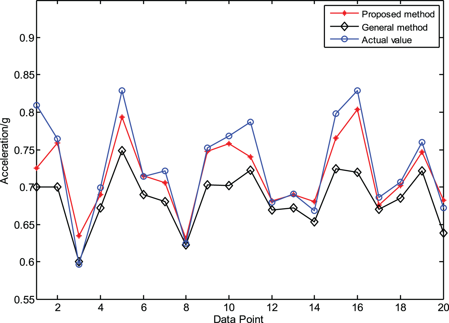
The comparison results for category A (red line for proposed method, black line for general method and blue line for actual value).
In order to verify the advantage of the proposed method in the prognosis of rolling bearing degradation performance, the general multivariable LS-SVM with a moving window is also utilized to predict the latter 20 RMS values. The training sample pairs and test sample are constructed according to Equations (12 to 14). The penalty coefficient and kernel parameter are also determined by the CSA algorithm. The results are also shown in Fig. 8.
In order to compare the performance of the two methods in detail, the root mean square error e RMSE , mean absolute error e MAE and cross-correlation coefficient R2 are presented in the Table 2.
The prognosis effect assessment
According to Fig. 8 and Table 2, the proposed multivariable LS-SVM over time slices can estimate the degradation trend much better and has higher prediction accuracy than that of the general method. Therefore, the results show that the multivariable LS-SVM over time slices outperforms the general multivariable LS-SVM.
To further study the robustness of the model, the samples are divided into three kinds of datasets, as in Table 3. The model construction is completed with a different number of training samples pairs to estimate the degradation trend. The result is also compared with that of the general multivariable LS-SVM.
The category of dataset
The result of category A is shown in Fig. 8, which proved the effectiveness of the proposed method. The results of category B and C are shown as Figs. 9 and 10, respectively. What is more, the evaluation indicators are presented in the Table 4 and Table 5.
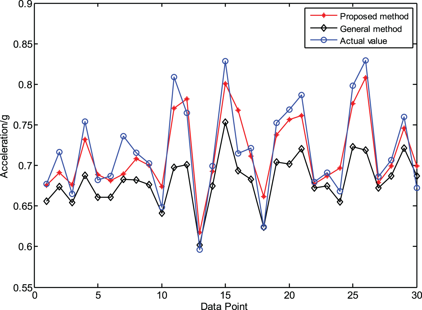
The results comparison for category B.
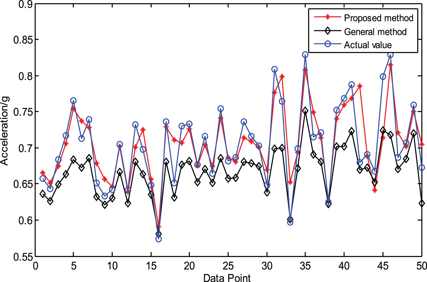
The results comparison for category C.
The prognosis effect assessment of category B
The prognosis effect assessment of category C
According to the results from categories A, B and C, the results further illustrate the effectiveness of the proposed method. The prediction accuracy obtained by the proposed method is higher than that of the general method.
With the reduction in the number of training samples, the accuracy of the degradation trend prediction is still maintained at a high level, which is much better than that of the general multivariable LS-SVM. Therefore, the proposed multivariable LS-SVM over time slices prediction model has good robustness and prediction accuracy and it can be used in the degradation trend prediction of rolling bearing.
In this paper, a new multivariable LS-SVM model is proposed for prediction of bearing performance degradation. Different features at different time slices are extracted to train the LS-SVM model by related analysis. The proposed model considers both the effects of signal volatility and multi-variables. In addition, to better track the dynamic changes of the signal, the model is updated with moving windows.
Compared with that of the general multivariable LS-SVM, experiments show that the proposed method can improve the prediction performance of the bearing degradation trend. What is more, as the number of training samples decreases, the prediction performance remains stable and robust. Therefore, the proposed model can be effectively applied to the prediction of bearing performance degradation.
Footnotes
Acknowledgments
This work is partially supported by National Natural Science Foundation of China (Grant nos. 51675035, 51405012) and the Open Fund of State Key Laboratory, Southwest Jiaotong University (TPL1603).