A mean-covariance decomposition method for battery capacity prognostics

Abstract

Lithium Ion batteries usually degrade to an unacceptable capacity level after hundreds or even thousands of charge and discharge cycles. The continuously observed capacity fade data over time and their internal structure can be informative for constructing capacity fade models. This paper applies a mean-covariance decomposition (MCD) modeling method using data within moving windows to analyze the capacity fade process. The proposed approach directly examines the variances and correlations in data of interest and reparameterize the correlation matrix in hyper-spherical coordinates using angle and trigonometric functions. To improve the interpretation of the prognostics model, the mean function is obtained based on physics of failure. Non-parametric methods are used to characterize the log variance and correlation through the number of cycles and time lags between capacity measurements, respectively. A numerical example is used to illustrate the superiority of the proposed method in prediction performance.

Keywords

Lithium ion battery capacity fading mean-covariance decomposition correlation matrix reparameterization physics of failure non-parametric moving window

1 Introduction

Lithium Ion batteries attract increasing attentions due to their high energy density and long lifetime. They are widely used in renewable power generation systems, aerospace systems, electric vehicle, etc. The failure of batteries could lead to the degraded performance or total failure of the system in some cases. Therefore, the diagnosis and prognostic of the performance and health condition of the lithium ion batteries becomes of great interests. Capacity, the maximum amount of electric charge that a fully charged battery can deliver, is one of three major performance indicators with the internal resistance and self-discharge. The lifetime of a battery is defined to end when its capacity reaches the 80% of the initial capacity in general. The loss of active Lithium ions during the micro-electrochemical reaction inside the battery during charge/discharge process causes the capacity fade. The uncertainties occurring during the chemical reactions result in the difficulties of the estimation of capacity fade under cycling usage. A variety of approaches to capture the randomness of the capacity fade are reported in recent literature, which can be categorized into data-driven and hybrid methods. Data-driven methods use the available and historical information to statistically and probabilistically derive decisions, estimates, and predicts the health and reliability [1]. Extensive work in the field of machine learning has been adopted for modeling batteries performance, such as Support vector machines (SVMs) [2 –5], Relevance vector machines (RVMs) [6, 7], k-nearest neighbor (kNN) [8], Artificial neural network (ANN) [9 –15]. The concept of entropy from the information theory is also used to model the battery capacity [16, 17], which would be effective to capture the information with non-standard cycling usage. Data-driven methods provide good fitted parsimonious models and accurate prediction, but it could be difficult to associate physical understanding to the variable in these models.

With development of sensing techniques, more physical understanding of batteries degradation mechanisms have been obtained. The physical failure mechanism can be utilized to assess battery reliability and predict the life time of batteries. Thus the hybrid method of data-driven and physics of failure is a significant interest in prognostic and health management. For example, based on the relationship between the terminal voltage and state of charge, model-based filter methods are developed to estimate the capacity of lithium ion batteries which are tested in closed circuits [18 –26]. The formation, growth, and repair of solid electrolyte interface (SEI) are the main reason for losing active lithium ions [27 –29], which occur during the electrochemical reactions of charge/discharge process. From the electrochemical viewpoint, the analytic models of capacity fade are studied [37, 38]. Due to the complexity of the chemical analysis, the uncertainties have not been well investigated. There is also some literature studying the lithium ion battery capacity from the degradation viewpoint. The degradation models aim to capture the factors that might affect the capacity of batteries. One of the major challenges of modeling degradation is to describe the uncertainties. Bayesian theory and statistical inference are used to model the uncertainties of the degradation [30 –36]. Based on the understanding in [35] about the longitudinal and between-sample uncertainties, this paper proposes a mean-covariance decomposition model to model these two types of uncertainties. The chemical analysis of SEI formation is used to formulate the basic model so that the result can have clear physical interpretation.

The remaining of this paper is organized as follows. Section 2 introduces the proposed mean-covariance decomposition modeling method. Section 3 reviews the analytic model of capacity and non-parametric models of log variance and correlation, followed by Section 4 where the analysis of the experiment illustrates the performance of the proposed method. Section 5 is the conclusion and future work.

2 Mean-covariance decomposition method

2.1 Mean-covariance decomposition in repeated measurements

In repeated measurements analysis, the observations of the same performance are obtained at certain time points. That is, the measurements y_i = (y_i1, y_i2, ⋯, y_{im
_i}) ^T collected from the ith subject, i = 1, 2, ⋯, observed at time t_i = (t_i1, t_i2, ⋯, t_{im
_i}) ^T. Under the assumption that y_i ∼ MVN (μ_i, Σ_i) where μ_i = (μ_i1, μ_i2, ⋯, μ_{im
_i}) ^T and Σ_i = D_iR_iD_i are the mean and covariance matrix for the ith subject. D_i = diag (σ_i1, σ_i2, ⋯, σ_{im
_i}) is the diagonal matrix with the standard deviation of the jth observation, σ_ij, j = 1, 2, ⋯, m_i. Then it is a natural and feasible idea to model the mean and covariance individualy [39]. The common modeling approaches of the mean μ are generalized regression models. For modeling the covriance Σ, there are two major difficulties: high dimensionality and positive definite constraints. To avoid these two difficulties, the concept of unconstrainted parameterization is applied to model the covariance matrix. Pinheiro et al. [40] summarized five unconstrained parameterizations of a covariance matrix, from which the Cholesky decomposition methods attract interets due to its high computation efficiency and easy interpretation of entities of the decomposed matrix. Pourahmadi [41] proposed the model of mean-variance-correlation based on the Cholesky decomposition of the covariance matrix, see Equation (1). Entities of the matrix T are interpreted as the auto-regression coefficients. In the framework of this mean-covariance decompostion, approaches to improve the interpretation of parameterization of covariance matrix with various forms of the Cholesky decomposition are explored. For example, Smith et al. [42] and Chen et al. [43] interpreted the entities of the decomposition matrix as one-step predictive coefficients and random effects coefficients, respectively.

$\begin{matrix} Σ^{- 1} & = & {TDT}^{'}, μ_{t} = m (x_{t}, β), \\ log σ_{t}^{2} & = & v (z_{t}, λ), φ_{t, j} = d (w_{j}, γ), \end{matrix}$ (1) where μ_t, $log σ_{t}^{2}$ are the mean and log variance of the observations at time t, while φ_t,j are the auto-regressive coefficients, i.e., entities of the decomposition matrix. x_t, z_t, and w_j represent the predictors, while β, λ, and γ are the parameters of the mean function, log variance, and correlation function, respectively.

The mixed effects model in [35] can be simplified as Equation (2), where y_i represent the measurements of the ith subject, X_i and Z_i are the covariates, and the errors are ɛ_i following MVN (0, σ²I). α and β_i are the fixed and random effects related parameters, respectively. $y_{i} = α X_{i} + β_{i} Z_{i} + ɛ_{i} .$ (2)

Under the assumption that β_i ∼ MVN (0, Σ_b), the measurements can be described in the form of y_i ∼ MVN (X_iα, Σ_i) with $Σ_{i} = Z_{i} Σ_{b} Z_{i}^{T} + σ^{2} I$ , which is consistent with the assumption of the mean-covariance decomposition modeling method, i.e., repeated measurements follow a multivariate normal distribution. The separation of the mean, variance, and correlation is desirable where the mean, variance, and correlation of measurements are modeled as a function of time-varying factors. The mean function indicates the longitudinal trend, while the variance and correlation function illustrate the between-subject random effects. For unbalanced repeated measurements/missing data, the mean and variance function in the proposed method can also be easily assessed. For the correlation function, if a subject is missing an observation, the correlation matrix R, which is unconstructed, can be just with the rows and columns corresponding to the missing observations [44]. Since the variance and correlation matrix are functions of time-varying predictive variables, the time-varying random effects, e.g., the individual effects of one subject might change over time, can also be captured. Therefore, predictions based on the proposed method would be more accurate, which is implemented through the multivariate normal distribution with the mean and dynamic covariance matrix obtained from the mean-variance-angle function.

2.2 Parameterization of correlation matrix using trigonometric functions

For the covariance matrix Σ_i of y_i, it can be decomposed as D_iR_iD_i based on the Cholesky decomposition, where D_i represents a diagonal matrix of variances and R_i is the corresponding correlation matrix. Since the correlation matrix is positive definite and symmetric with off-diagonal entities between -1 and 1, R_i can be future decomposed as $T_{i} T_{i}^{'}$ , where T_i is the lower triangular matrix, see Equation (3). Jaeckel et al. [45] proposed a trigonometric parameterization of this decomposition matrix T_i of the correlation matrix via the Givens rotation, which is also investigated by Creal et al. [46] and Zhang et al. [47], see Equation (4). $Σ_{i} = D_{i} R_{i} D_{i}, R_{i} = T_{i} T_{i}^{'} .$ (3) $\begin{matrix} R_{i} & = & (ρ_{ijk})_{j, k = 1}^{m_{i}}; \\ T_{i 11} & = & 1; T_{ij 1} = cos (φ_{ijk}), 1 \leq j \leq m_{i}; \\ T_{ijk} & = & {\begin{matrix} cos (φ_{ijk}) \prod_{i = 1}^{k - 1} sin (φ_{ijl}), & 2 \leq k < j \leq m_{i}; \\ \prod_{i = 1}^{k - 1} \sin (φ_{ijl}), & k = 2, \dots, m_{i} . \end{matrix} \end{matrix}$ (4) where m_i represents the number of observations. Let e_j, j = 1, ⋯, m_i be canonical basis and φ_ijk is the angle between the projection of the jth column of T_i, denoted as T_ij, on the subspace of {e_j, e_k} and e_k. $T_{ij} = \prod_{k = 1}^{j - 1} G (k, k + 1; φ_{ijk}) e_{1}$ , where G (i, j ; φ) is the Givens rotation and G (i, j ; φ) is different from m-dimensional identity matrix with the elements of G_ii = cos φ, G_ij = - sin φ, G_ji = sin φ, and G_jj = cos φ. Based on Equation $R_{i} = T_{i} T_{i}^{'}$ and (4), Equation (5) can be derived [47] which maps from a general correlation matrix R_i to the angles φ_ijk. φ_ijk is unconstrained in the range of [0, π) and can be driven by the time-varying predictive variables, such as cycle lags. Then entities in the correlation matrix can be modeled as a function of time-varying factors based on Equation (5). Moreover, modeling φ_ijk for the correlation matrix can also reduce the number of time-varying factors, when the dimensionality of y_i increases [46]. Therefore, the model with mean-variance-angles function can be expressed in Equation (6). $\begin{matrix} φ_{ijk} & = & arccos (T_{ijk} / \prod_{l = 1}^{k - 1} sin (arccos (φ_{ijl}))), \\ ρ_{ijk} & = & \sum_{l = 1}^{k - 1} [cos (φ_{ijl}) cos (φ_{ikl}) \\ \prod_{t = 1}^{l - 1} sin (φ_{ijt}) sin (φ_{ikt})] \\ + cos (φ_{ijk}) \prod_{l = 1}^{k - 1} sin (φ_{ijl}), 1 \leq k < j \leq m_{i} . \end{matrix}$ (5) $μ_{i} = X_{i} α, log σ_{i}^{2} = Z_{i} β, φ_{ijk} = W_{ijk} λ,$ (6) where φ_ijk is the angle between the projection of T_ij on the subspace of {e_j, e_k} and e_k, X_i, Z_i, and W_ijk are covariates of mean function, log variance function, and angles functions for correlation coefficients, respectively.

2.3 Selection of covariates

In Equation (6), X_i are the covariates that are used to model the mean of the measurements. Under the assumption that repeated measurements follow a multivariate normal distribution, repeated measurements of various samples can be the mean of this multivariate distribution. The selection of X_i might mainly depend on the analytic model of the degradation process. For the battery capacity degradation, it is a natural idea that covariates could be selected from the factors affecting SEI formation during the electro-chemical reaction, such as the number of cycles, charge and discharge rate, temperature, etc. These factors are also good candidates of Z_i, the covariates of the log variance of the jth observations. The correlation between measurements y_i and y_j decays over the time difference between the measurements. Thus W_ijk should include time varying covariates that depends on time t_ik and t_ij as it is capturing the correlation between the responses at these two measurement time.

2.4 Parameters estimation

2.4.1 Moving-window scheme

It is evident that the strength of the “impact” that one measurement has on another measurement will depend on average decay as a function of their corresponding time lag in the time sequence. For a relatively slow degradation process, such as lithium ion battery capacity fading, the previous observations have a weak effect on the current observation and might distort the prediction. The moving-window method is to use information from the most recent observations to predict the future values. Models based on a large window provide the less accurate information along the perturbation direction, while those based on a small window are effective to obtain the pertinent information of perturbation direction. However, the small moving window might not be robust with high noise level [48]. The optimal length of a moving window in this paper is determined using the prognostic performance in the term of the mean absolute deviation (MAD) based on one-step-ahead predicted value and actual observed value. The core of calculating MAD of one moving window is to use a constant size of historical data to predict the next one value and obtain the residual. The details of the four-steps of determining moving window length can be found in [35]. Moreover, the moving-window scheme with the constant length simplifies the modeling of the correlation which is the function of the difference between the measured time being the same for a certain length of the moving window.

2.4.2 Parameters in mean-variance-angles function

For each moving window, parameters in Equation (6) are estimated through balancing the measurement fit and the model complexity. The basic form of functions of mean, log variance, and angles for correlations can be obtained from the physical understanding and empirical functions. For example, the chemical analytic model from [29, 37] can be referred as the basic model of mean, which is discussed in Section 3.

3 Lithium Ion battery capacity fade model

Section 2 describes the mean-covariance decomposition modeling method to analyze the battery capacity fade of Lithium ion batteries, where the basic models of the models of mean, log variance, and angles for correlations are expected to extract from the physical failure model or empirical model. This section reviews one of the recent major analytic models of formation and growth of solid electrolyte interphase (SEI) that causes the battery capacity fading in the cycling usage.

3.1 Mean function

The chemical degradation mechanism has been widely recognized as one of the main causes of losses of active lithium ions, especially the SEI formation. The capacity fading analysis models based on chemical degradation mechanism attract interests. This paper develops the basic form of the mean function by incorporating the chemical degradation model in [37]. The four scenarios of active lithium ion losses are combined: SEI formation at the first cycle, SEI thickness growth on the original surface, SEI formation due to crack propagation, and SEI thickness growth on the cracked surface, see Equation (7).

$\begin{matrix} \hat{Q} & = & 1 + \frac{(2 - m) BA L_{0}}{C} ((1 - CN)^{2 / (2 - m)} \\ - (1 - C)^{2 / (2 - m)}), \end{matrix}$ (7) where $\hat{Q}$ represents the fraction capacity and N is the number of cycles. m, C, A, B, C, m and L₀ are parameters determined by the material of batteries [49]. To enable this model to analyze various types of lithium ion batteries, Equation (7) can be simplified into a general form. It is reasonable to rewrite Equation (7) into a polynomial function of the number of cycles, see Equation (7).

$\begin{matrix} Q (N) & = & a_{n} N^{2 / (2 - m)} + a_{n - 1} N^{2 / (2 - m) - 1} \\ + \dots + a_{1} N + a_{0}, \end{matrix}$ (8) where Q (N) is the battery capacity at cycle N, a_i, i = n, ⋯, 1 are the coefficients of the polynomial terms and a₀ represents the constant. Based on the above analysis, the mean of Li-ion batteries capacity degradation process, αX_i, can be modeled as a polynomial degradation function over charge/discharge cycles.

3.2 Log variance and angles function

Due to the lack of physical understanding of log variance and correlation of the capacity degradation process, the log variance $log σ_{i}^{2}$ and angles φ_ijk are estimated through non-parametric methods. This paper uses the support vector machine (SVM) regression with ∊-insensitive loss function in the consideration its advantages in efficiency, accuracy, and robustness [50]. Support vectors are trained in SVM regression so that the data points lie in between the two borders of the margin which is maximized under suitable conditions to avoid outliers inclusion. SVM regression is formulated as controlling the model complexity and margins through the squared norm of the parameters vector and loss function respectively. Take a general regression model y = w ^Tg ( x ) + w₀ for example. In this model, g ( x ) is a function mapping each input x to a higher dimensional space, w = (w₁, w₂, …, w_m) ^T denotes a set of linear weights connecting the feature space g ( x ) to the output y, and w₀ is the constant. Parameters w and w₀ can be estimated through minimizing $w, w_{0}, ξ, ξ^{*} \frac{1}{2} ∥ w ∥^{2} + C \sum_{i = 1}^{m} (ξ_{i} + ξ_{i}^{*})$ with constraints of $w^{T} g (x_{i}) + w_{0} - y_{i} \leq ∊ + ξ_{i}, y_{i} - w^{T} g (x_{i}) - w_{0} \leq ∊ + ξ_{i}^{*}, ξ_{i}, ξ_{i}^{*} \geq 0$ , where slack variables ξ_i and $ξ_{i}^{*}$ penalize predictions out of the ∊-intensive tube, and the penalty parameter C > 0 determines the trade off between the flatness of the function and the amount up to which deviations larger than ∊ are tolerated. The above optimization problem can be transformed into the dual problem as $\sum_{i = 1}^{n_{sv}} (a_{i} - a_{i}^{*}) g (x_{i})^{T} g (x) + w_{0}$ with the constraint of $0 \leq a_{i}, a_{i}^{*} \leq C$ where $a_{i}, a_{i}^{*}, i = 1, \dots, n_{SV}$ are the Lagrange multipliers and n_sv is the number of support vectors. The inner product g (x_i) ^Tg (x) can be integrated as a kernel function K (·). The choice of the kernel function depends on the characteristics of the data. For the log variance and angle functions, the Gaussian kernel K (x_i, x) = exp(γ ∥ x_i - x ∥ ²) is used for the practical purpose. Usually the set of the penalty parameter C in the loss function and γ in the Gaussian kernel is given on the interval [2^-5, 2¹⁵] and [2^-15, 2³]. The grid-search method is often to test various pairs of (C, γ) over cross-validation randomized samples and the pair with the minimal residual is selected. However, the grid search is very inefficient when the large scale data set is used as input or small grid is required. This paper uses random search where multiple random sampled candidates of C and γ are used for cross-validation. One of the major advantages of random search is to decrease the computation time so that a large range of C and γ can be tested [51, 52]. To model log variances and angles in MCD, their covariates, such as the number of cycles and cycle lags, are considered as inputs of the kernel functions.

Fig.1

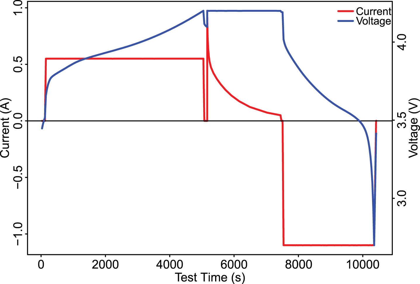
The profile of voltage and current in a charge/discharge cycle.

4 Experimental results

4.1 Experimental data

This section presents the cycling test and the result analysis using the proposed mean-covariance decomposition modeling method. Four lithium ion batteries, CS2_35, CS2_36, CS2_37, and CS2_38, are tested in room temperature under constant-current-constant-voltage (CCCV) charge/discharge profile. The cycling test is conducted with the following setting: 1) the constant current charge rate is 1C; 2) the cutoff voltage is 4.2 V; 3) The voltage is 4.2 for the constant voltage charge; 4) the discharge rate is 1C; 5) the discharge cutoff voltage is 2.5 V. Typical voltage and current of a Lithium ion battery cell during a charge/discharge cycle are shown in Fig. 1. Table 1 and Fig. 2 summarize the experimental results where the capacity fade profile over cycles is reported.

Table 1
Summary of experiment data

Sample Discharge rate Number of cycles Cycle to failure

CS2_35 1C 930 645

CS2_36 1C 970 549

CS2_37 1C 1036 625

CS2_38 1C 1050 672

Sample	Discharge rate	Number of cycles	Cycle to failure
CS2_35	1C	930	645
CS2_36	1C	970	549
CS2_37	1C	1036	625
CS2_38	1C	1050	672

Fig.2

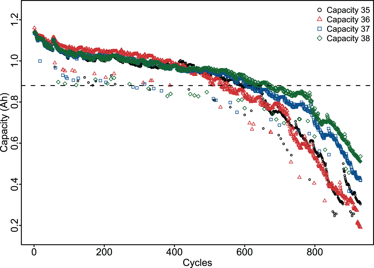
The capacity fade of tested batteries over cycles.

4.2 Modeling and analysis

4.2.1 Modeling the mean of capacity

Factors that affect the electrochemical reactions during the charge/discharge process are natural candidates of covariates of the mean and covariance functions. As discussed in Section 3, the basic form of the mean function is a polynomial function of the number of cycles under a CCCV charge/discharge profile at a constant temperature. Based on the basic form of the mean function discussed in Section 3, the cubic function of the number of cycles is selected to model the mean by balancing the measurement of fit and measurement of complexity, see Equation (9) and Fig. 3. Parameters are determined by balancing the residuals and test errors. The training data and test data in this work is 80% and 20%. The root-mean-square error (RMSE) of this predicted model is 0.0147.

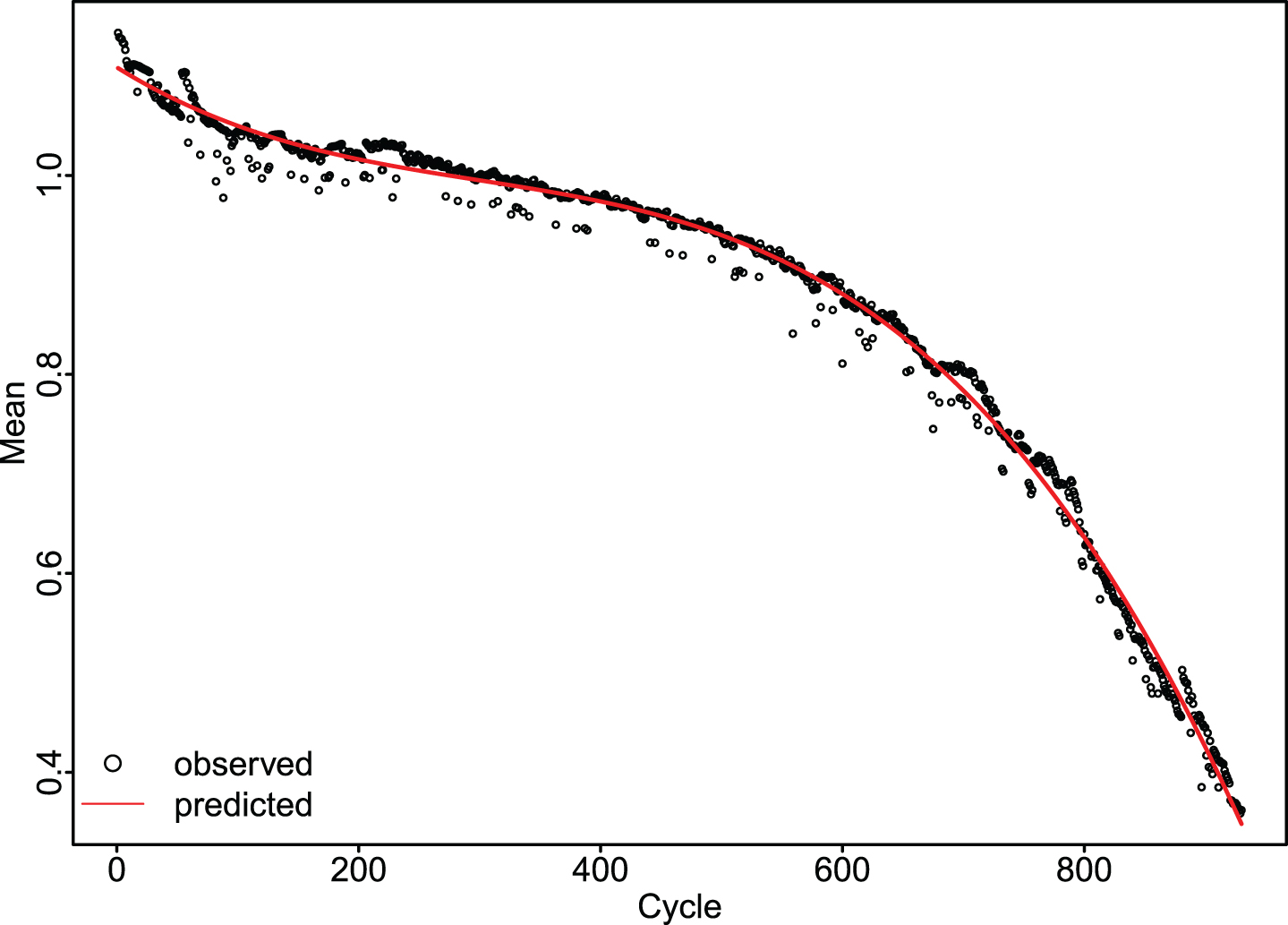
$\begin{matrix} μ & = & 1.109 - 7.679 \times 10^{- 4} N \\ + 1.947 \times 10^{- 6} N^{2} - 2.171 \times 10^{- 9} N^{3}, \end{matrix}$ (9) where μ is the mean function of the capacity fading and N is the number of cycles.

Fig.3

The prediction model for the mean.

4.2.2 Modeling of log variance and correlation

The variance of measurements at each cycle and their correlations are obtained based on the Chelosky decomposition, based on Equations (3) and (4). The prerequisite of the Chelosky decomposition of the correlation matrix is that this matrix is symmetric and positive definite. However, a correlation matrix based on the historical data is not always non-negative definite due to missing data, noises and linearity of components. A broken correlation matrix with some negative eigenvalues with small absolute values can be fixed. A simulation-based method is used to create a positive definite matrix out of a broken correlation matrix, where the small negative eigenvalues are replaced by normally distributed random variables with the mean of 0 and small variance [53]. Based on Equation (6), the log variance and angles φ_ijk can be obtained, see Figs. 4 and 5.

Fig.4

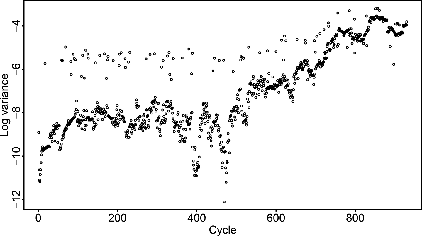
The log variance versus the number of cycles.

Fig.5

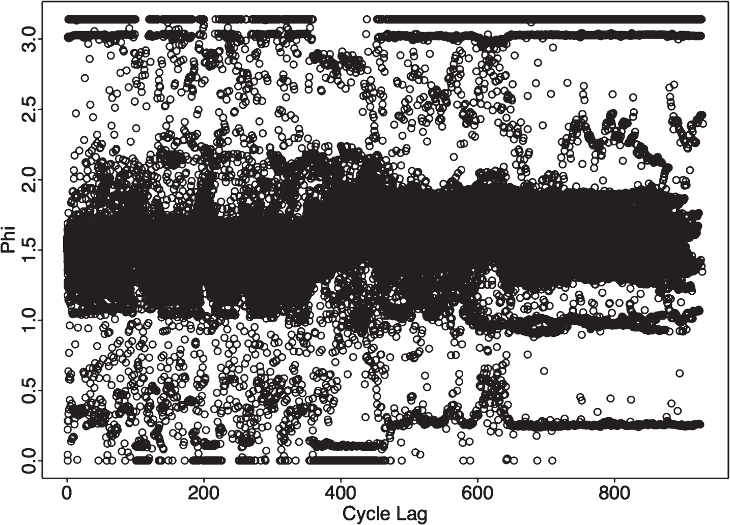
The angles versus the cycle lag.

For the log variance function, the number of cycles is also a natural choice. The angle function has a unique relationship with the entities of the correlation matrix. Thus the cycle-lag, the time difference between measurements, is selected as the covariate of the angle function. Statistical tests are implemented to demonstrate the statistical significance of the selected covariate to the log variance and angle function for correlations. It is difficult to detect equality of variance since only one observation for the log variance is available. To investigate the variance of the log variance over cycles, the bootstrapping method is employed to generate samples. The bootstrapping samples of any three batteries capacity observations are randomly sampled from four batteries, and log variances of three capacity observations at each cycle are calculated. The ANOVA assumptions of homoscedasticity and residual normality in the log variance are checked. It can be concluded that these two assumptions are violated with significant p-values, see Table 2 check. In addition, sample sizes of the angle functions over cycles are unbalanced due to which the one-way AVONA test is too sensitive to inequality of variances and non-applicable. Therefore, the nonparametric test of Friedman test is employed considering its robustness in dealing with non-normality, heterscedasticity, and outliers. The null hypothesis of the Friedman test is assigned as that there are no differences between the predictive variables. If p-value is significant, it can be concluded that at least 2 of variables are significantly different from each other. The results of Friedman tests over log variance and angle functions for correlations are shown in Table 3 fried, where p-values for both log variance and angles are significant. We can reject the null hypothesis of tests for both log variances and angles. It can be concluded that the number of cycles is statistically significant to log variance and cycle lags are statistically significant to angles.

Table 2

Assumptions of equality of variance and residual normality for the log variance

Test of equality of variance- Studentized Breusch-Pagan test
BP	325.52
Degrees of free	1
p-value	<2.2e - 16
Test of residual normality - Shapiro-Wilk normality test
W	0.85919
p-value	<2.2e - 16

Table 3

Friedman test of log variance and angles for correlations

log variance
Chi-squared	626.53
Degrees of freedom	3
p-value	<2.2e - 16
Angle functions for correlations
Chi-square	28570
Degrees of freedom	928
p-value	<2.2e - 16

4.2.3 Determining the optimal moving-window length

As discussed in Section 1, the MAD is the performance index of the length of the moving window. Considering the end cycle of life, the optimal size of moving-window of the proposed method is 46 with the minimum mean absolute deviation (MAD), 1.215e - 06, while that of the mixed effects model is 195 with MAD of 0.0014 [35], see Fig. 6. Compared the MAD of various lengths of moving window of the proposed method and the mixed effects model, it can be concluded that a smaller amount of historical data to predict future values for the proposed method than mixed effects model needs and the accuracy of prediction is improved with a lower MAD. When taking all the available test data into account, the deviation of the prediction based on the mixed effects model increases due to high variance, see Fig. 6.

Fig.6

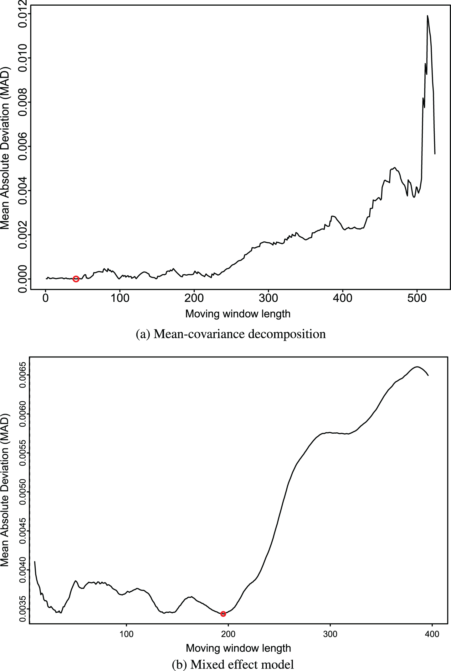
The optimal moving window of mean-covariance decomposition and mixed effect model.

Within a moving window, SVM regression with ∊-regression is used to model the log variance and angles [54]. The number of cycles and cycle lag are selected as the candidat inputs of kernel functions for the SVM regression of log-variances and angles, according to the statistical test result in Section 4.2.2. Without losing generality, polynomials of the number of cycles are considered as the inputs of kernel functions of the log variance function, while polynomials of cycle lags are considered as the inputs of kernel functions of angles. Figures 7 and 8 show SVM regression models of the log variance and angles of one of moving windows (495-540) and their prediction performance in terms of root mean square error (RMSE).

Fig.7

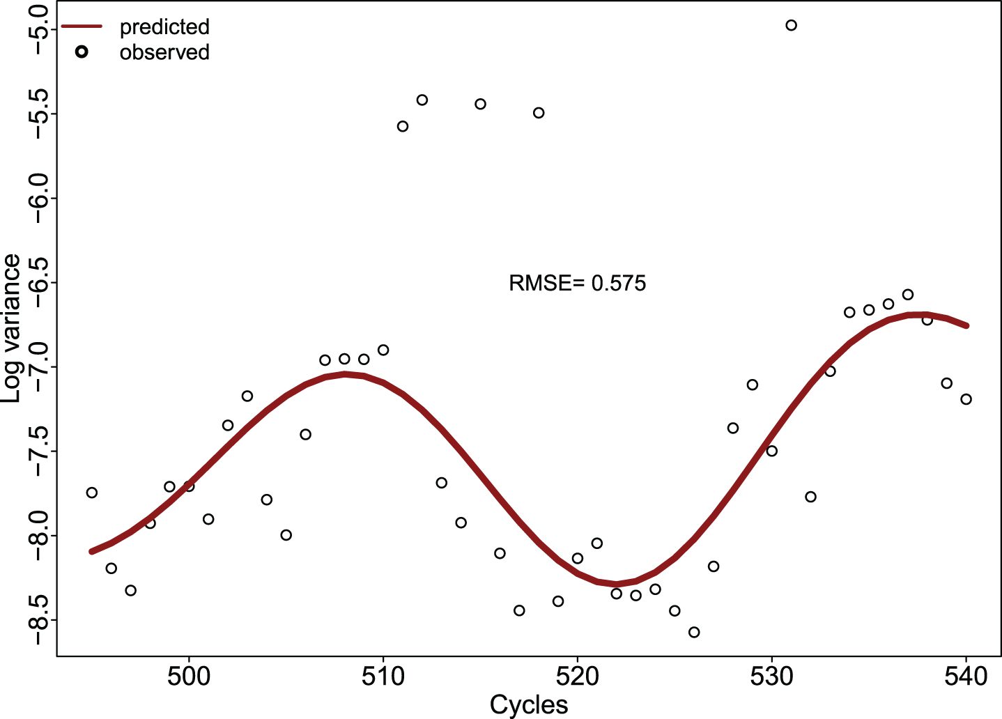
The actual and predicted log variance.

Fig.8

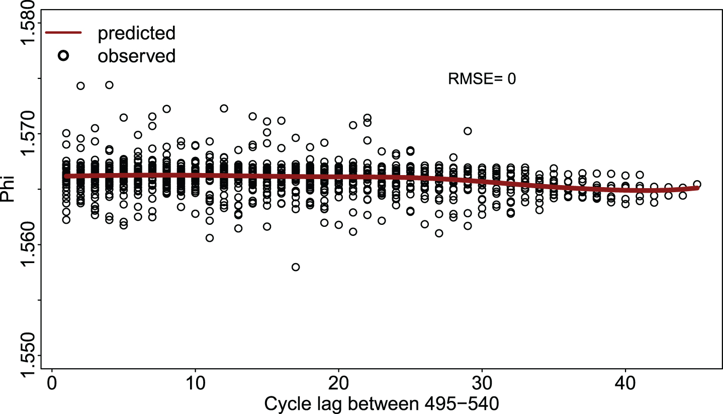
The actual and predicted angles versus the cycle lags.

4.2.4 Performance assessment

To have a better understanding of the cycle to failure estimation, the mean-covariance decomposition model with the optimal moving window length of 46 is used to predict the capacity around the last cycles. Considering the end life cycles shown in Table 1, data of the first 540 cycles is used to predict the cycle to failure at which the capacity of batteries is less or equal to 80% of the initial capacity. The prediction based on the proposed method uses based on the optimal window. That is, the predictions of the capacity at cycle 541 is predicted based on the historical capacity data at cycle 495 to 540, and that at cycle 542 relies on 496 to 541, and so on. The prediction of future values is provided in the form of a multivariate normal distribution, where each variate, the prediction of the capacity, follows a normal distribution. The predicted capacity and the 90% confidence interval are shown in Fig. 9, where capacity measurements of CS2_35, CS2_36, CS2_37, and CS2_38, the means of both MCD and mixed effect model are demonstrated. To compare the prediction performance of MCD and mixed effect model, the average width of 90% confidence interval of 0.058, while that of the mixed effects model is 0.064. That is, the prediction based on mean-covariance decomposition method is more accurate compared with that of the model proposed in [35].

Fig.9

Performance comparison of the proposed method and the mixed effects model.

4.2.5 Cycle to failure prediction

Given the number of cycles, the capacity can be simulated under the MCD model for a large number of iterations. By counting the percentage of the simulated capacities less than the specified failure threshold, i.e., 0.88 Ah, cycle to failure distribution can be obtained, see Fig. 10, where the average of observed cycle to failure of four batteries is 623. It turns out that the mean of the cycle to failure is 635 and the standard deviation is 14.3.

Fig.10

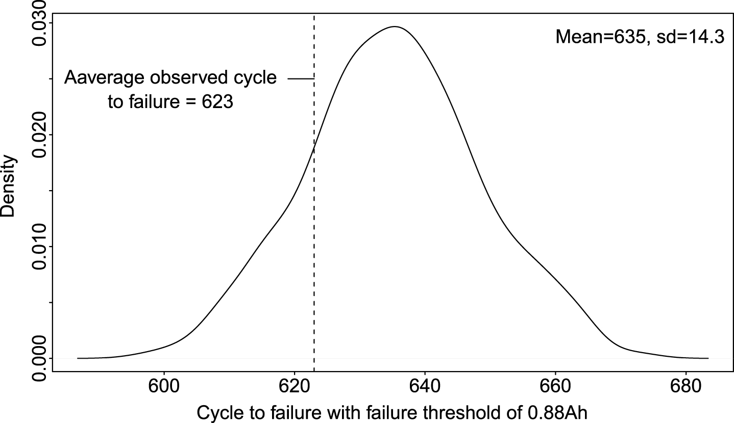
Cycle to failure estimation and the observed average cycle to failure with D_F = 0.88Ah.

5 Conclusion

A mean-covariance modeling method is proposed to model the longitudinal and between-sample uncertainties. Through the covariance matrix of the multivariate normal distribution of the repeated measurement, mean-covariance decomposition can effectively deal with unbalance data through decomposed covariance matrix and the time-vary random effects. With the characteristics of the correlation matrix, a trigonometric function is used to reparameterize the correlation matrix, which can reduce the time-varying factors of the correlation matrix. To improve the interpretation of the degradation model, the analytic model from the electrochemical viewpoint is employed as the basic form of the mean function. For the slow degradation process, the moving-window scheme is used to include the most recent information for predictions. Within the optimal moving window, the parameters in the mean-covariance models are estimated through balancing the goodness-of-fit of the capacity data and the model complexity. Compared with the mixed effects model, the proposed method needs fewer historical data with the moving window with smaller length, which improves the accuracy of the prediction. The cycle to failure can be easily obtained through simulations.

References

Pecht

, Prognostics and health management of electronicsJohn Wiley & Sons, 2008.

Hansen

and Wang

, Support vector based battery state of charge estimator, Journal of Power Sources141 (2005), 351–358.

Shi

, Zhang

and Cui

, Estimation of battery state of chargeusing v-support vector regression algorithm, International Journal of Automotive Technology9 (2008), 759–764.

Pattipati

, Sankavaram

and Pattipati

, System identification and estimation framework for pivotalautomotive battery management system characteristics, IEEE Transactions on Systems, Man, and Cybernetics, Part C (Applications and Reviews)2011, pp. 1–16.

Nuhic

, Terzimehic

, Soczka-Guth

, Bucholz

and Dietmayer

, Health diagnosis and remaining useful life prognostics of lithium-ion batteries using data-driven methods, Journal of Power Sources239 (2013), 680–688.

Saha

, Goebel

, Poll

and Christophersen

, Prognostic methods for battery health monitoring using aBayesian framework, IEEE Transactions on Instrumentation and Measurement58 (2009), 291–296.

, Jain

, Schmidt

, Strief

and Sullivan

, Online estimation of lithium-ion battery capacity usingsparse Bayesian learning, Journal of Power Sources289 (2015), 105–113.

, Jain

, Zhang

, Schmidt

, Gomadam

and Gorka

, Data-driven approach based on particle swarmoptimization and k-nearest neighbor regression for estimating capacity of lithium-ion battery, Applied Energy129 (2014), 49–55.

Shen

, Chan

, Lo

and Chau

, A new battery available capacity indicator for electric veihles using neral network, Energy Conversion Management43 (2002), 817–826.

10.

Lee

, Wang

and Kuo

, Soft computing for battery stateof-charge (BSOC) estimation in battery stringsystems, IEEE Transaction on Industrial Electronics55 (2005), 229–239.

11.

, Wang

, Su

and Lee

, A merged fuzzy neural network and its applications in battery state-of-charge estimation, IEEE Transaction on Energy Conversion22 (2007), 697–708.

12.

Chang

, Bai

and Cao

, State of charge estimation based on evolutionary neural network, Energy Conversion Management49 (2008), 2788–2794.

13.

Weigert

, Tian

and Lian

, State of charge prediction of batteries and battery supercapacitor hybrids usingartificial neural networks, Journal of Power Sources196 (2011), 4061–4064.

14.

Eddaheck

, Briat

, Bertrand

, Deletage

and Vinassa

, Behavior and state of health monitoring of Li-ionbatteries using impedance spectroscopy and recurring neural networks, International Journal of ElectricalPower Energy Systems42 (2012), 487–494.

15.

Kim

, Lee

and Cho

, Complementary cooperation algorithm based on DFKF combined with pattern cognition forSOC/capacity estimation and SOH prediction, IEEE Transaction on Power Electronics27 (2012), 436–451.

16.

Sun

, Jou

and Wu

, Auxiliary diagnosis method for leadacid battery health based on sample entropy, Energy Conversion and Management50 (2009), 2250–2256.

17.

Widodo

, Shim

, Caesarendra

and Yang

, Intelligent prognostics for battery health monitoring based onsample entropy, Expert Systems with Applications38 (2011), 11763–11769.

18.

Plett

, Extended Kalman filtering for battery management systems of LiPB-based HEV battery packs: Part3. Stateand parameter estimation, Journal of Power Sources134 (2004), 277–292.

19.

Plett

, Sigma-point Kalman filtering for battery management systems of LiPB-based HEV battery packs: Part 2.simultaneous state and parameter estimation, Journal of Power Sources161 (2006), 1369–1384.

20.

Lee

, Nam

and Cho

, Li-ion battery SOC estimation method based on the reduced order extended Kalmanfiltering, Journal of Power Sources174 (2007), 9–15.

21.

Lee

, Kim

, Lee

and Cho

, State-of-charge and capacity estimation of lithium ion battery using a newopen-circuit voltage versus state-of-charge, Journal of Power Sources (2008), 1367–1373.

22.

Saha

and Goebel

, Modeling Li-ion battery capacity depletion in a particle filtering framework, Proceedings of annual conference of the PHM Society

San Diego, CA

2009.

23.

Sun

, Hu

, Zou

and Li

, Adaptive unscented Kalman filtering for state of charge estimation of alithium-ion battery for electric vehicles, Energy36 (2011), 3531–3540.

24.

, Youn

and Chung

, A multiscale frame work with extendedKalman filter for lithium-ion battery SOC and capacity estimation, Applied Engergy92 (2012), 694–704.

25.

, Williad

, Chao

and Pecht

, State of charge estimation for electric vehicle batteries usin gunscented kalman filtering, Microeletronics Reliability53 (2013), 840–847.

26.

Xiong

, Sun

, Chen

and He

, A data-driven multi-scale extended Kalman filtering based parameter andstate estimation apparoache of lithium-ion battery in electric vehicles, Applied Energy113 (2014), 463–476.

27.

Vetter

, Novák

, Wagner

, Veit

, Möller

, Besenhard

, Winter

, Wohlfahrt-Mehrens

Vogler

and Hammouche

, Ageing mechanism in lithium-ion batteries, Journal of Power Sources147(2005), 269–281.

28.

Yan

, Xia

, Su

, Zhou

, Zhang

and Zhang

, Phenomenologically modeling the formation and evolution ofthe solid electrolyte interface on the graphite electrode for lithiumion batteries, Journal of Power Sources53 (2008), 7069–7078.

29.

Pinson

and Bazant

, Theory of SEI formation in rechargeable batteries: Capacity fade, accelerated aging andlifetime prediction, Journal of The Electrochemical Society160 (2013), A243–A250.

30.

Ning

, Haran

and Popov

, Capacity fade study of lithiumion batteries cycled at high discharge rate, Journal of Power Sources117 (2003), 160–169.

31.

Safari

, Morcrette

, Teyssot

and Delacourt

, Multimodal physics-based aging model for life prediction ofLi-Ion batteries,, Journal of The Electrochemical Society156 (2009) A145–A153.

32.

Jin

, Matthews

and Zhou

, A Bayesian framework for online degradation assessment and residual life prediction of secondary batteries in spacecraft, Reliability Engineering and System Safety113(2013), 7–20.

33.

Liu

, Pang

, Zhou

, Peng

and Pecht

, Prognostics for state of health estimation of lithium-ion batteries based on combination Gaussian process functional regression, Microelectronics Reliability53 (2013), 832–839.

34.

, Williard

, Osterman

and Pecht

, Prognostics of lithium-ion batteries based on Dempster-Shafertheory and the Bayesian Monte Carlo method, Journal of Power Sources196 (2013), 10314–10321.

35.

Guo

, Li

and Pecht

, A Bayesian approach for Li-Ion battery capacity fade modeling and cycles to failureprognostics, Journal of Power Sources281 (2015), 173–184.

36.

Muenzel

, A multi-factor battery cycle life prediction methodology for optimal battery management, ACM, Proceedings of the 2015 ACM Sixth International Conference on Future Energy Systems2015.

37.

Deshpande

, Verbrugge

, Chen

, Wang

and Liu

, Battery cycle life prediction with coupled chemicaldegradation and fatigue mechanics.

38.

Degradation-limiting optimization of battery energy storage systems operationMaster’s thesis, ETH Zurich, Zurich, Switzerland, 2013.

39.

Sklar

Fonctions de répartition á n dimensions et leurs marges, Publications de L’Institut deStatistique de L’Université de Paris 8, (1959) pp. 229–231Paris.

40.

Pinheiro

and Bates

, Unconstrained parameterizations for variance-covariance matrices, Statistics and Computing6 (1996), 289–296.

41.

Pourahmadi

, Joint mean-covariance models with applications to longitudinal data: Unconstrainedparameterisation, Biometrika86 (1999), 677–690.

42.

Smith

and Kohn

, Parsimonious covariance matrix estimation for longitudinal data, Journal of theAmerican Statistical Association97 (2002), 1141–1153.

43.

Chen

and Dunson

, Random effects selection in linear mixed models, Biometrics59 (2003), 762–769.

44.

Cnaan

, Laird

and Slasor

, Tutorial in biostatistics: Using the general linear mixed model to analyseunbalanced repeated measures and longitudinal data, Statistics In Medicine16 (1997), 2349–2380.

45.

Jaeckel

and Rebonato

, The most general methodology for creating a valid correlation matrix for riskmanagement and option pricing purposes, Journal of Risk2.2 (1999), 17–28.

46.

Creal

, Koopman

and Lucas

, A dynamic multivariate heavy tailed model for time-varying volatilities andcorrelations, Journal of Business and Economic Statistics29 (2011), 552–563.

47.

Zhang

, Leng

and Tang

, A joint modeling approach for longitudinal studies, Journal of the RoyalStatistical Society: Series B (Statistical Methodology)77 (2015), 219–238.

48.

Morita

, Shinzawa

, Tsenkova

, Noda

and Ozaki

, Computational simulations and a practical applicationof movingwindow two-dimensional correlation spectroscopy, Journal of Molecular Structure799 (2006), 111–120.

49.

Suresh

, Fatigue of materialsCambridge University Press1998.

50.

Cortes

and Vapnik

, Support-vector network, Machine Learning20 (1995), 1–25.

51.

Bergstra

and Bengio

, Random search for hyper-parameter optimization, Journal of Machine LearningResearch13 (2012), 281–305.

52.

Cleveland

, Robust locally weighted regression and smoothing scatter-plots, Journal of the AmericanStatistical Association74 (1979), 829–836.

53.

Brissette

, Khalili

and Leconte

, Efficient stochastic generation of multi-site synthetic precipitationdata, Journal of Hydrology345 (2007), 121–133.

54.

Dimitriadou

, Hornik

, Leisch

, Meyer

and Weingessel

, The R project forstatistical computing, SVM, e1071 Package2004.

A mean-covariance decomposition method for battery capacity prognostics

Abstract

Keywords

1 Introduction

2 Mean-covariance decomposition method

2.1 Mean-covariance decomposition in repeated measurements

2.4 Parameters estimation

2.4.1 Moving-window scheme

2.4.2 Parameters in mean-variance-angles function

3 Lithium Ion battery capacity fade model

3.1 Mean function

4.1 Experimental data

Table 1 Summary of experiment data Sample Discharge rate Number of cycles Cycle to failure CS2_35 1C 930 645 CS2_36 1C 970 549 CS2_37 1C 1036 625 CS2_38 1C 1050 672

4.2.1 Modeling the mean of capacity

References

Table 1
Summary of experiment data

Sample Discharge rate Number of cycles Cycle to failure

CS2_35 1C 930 645

CS2_36 1C 970 549

CS2_37 1C 1036 625

CS2_38 1C 1050 672