Canonical variate analysis,probability approach and support vector regression for fault identification and failure time prediction

Abstract

Reciprocating compressors are widely used in oil and gas industry for gas transport, lift and injection. Critical compressors that compress flammable gases and operate at high speeds are high priority equipment on maintenance improvement lists. Identifying the root causes of faults and estimating remaining usable time for reciprocating compressors could potentially reduce downtime and maintenance costs, and improve safety and availability. In this study, Canonical Variate Analysis (CVA), Cox Proportional Hazard (CPHM) and Support Vector Regression (SVR) models are employed to identify fault related variables and predict remaining usable time based on sensory data acquired from an operational industrial reciprocating compressor. 2-D contribution plots for CVA-based residual and state spaces were developed to identify variables that are closely related to compressor faults. Furthermore, a SVR model was used as a prognostic tool following training with failure rate vectors obtained from the CPHM and health indicators obtained from the CVA model. The trained SVR model was utilized to estimate the failure degradation rate and remaining useful life of the compressor. The results indicate that the proposed method can be effectively used in real industrial processes to perform fault diagnosis and prognosis.

Keywords

Condition monitoring canonical variate analysis cox proportional hazard model support vector regression

1 Introduction

Modern industrial facilities such as natural-gas processing plants are becoming increasingly complex and large-scale as a result of increased mechanization and automation. The complexity of large-scale industrial facilities makes it difficult to build first-principle dynamic models for health monitoring and prognostics [9]. The existing condition monitoring approaches for industrial processes are typically derived from routinely collected system operating data. With the rapid growth and advancement in sensing and data acquisition technologies, long-term continuous measurements can be taken from different sensors mounted on machinery systems. However, using condition monitoring data for reliable faults diagnosis and prognosis remains a challenge for researchers and engineers.

A number of multivariate statistical techniques have been developed based on condition monitoring data for diagnostic and prognostic health monitoring, such as filtering based models [6], multivariate time-series models [11] and neural networks [22]. Some of the key challenges in the implementation of these techniques are strongly correlated variables, high-dimensional data, changing operating conditions and inherent system uncertainty [4]. Recent developments of dimensionality reduction techniques have shown improvements in identifying faults from highly correlated process variables. Conventional dimensionality reduction methods are principal component analysis (PCA) [10], independent component analysis (ICA) [1] and partial least-squares analysis (PLSA) [21]. These basic multivariate methods have been proven to perform well under the assumption that process variables are time-independent. However, this assumption might not hold true for real industrial processes (especially chemical and petrochemical processes) because sensory signals affected by noises and disturbances often show strong correlation between the past and future sampling points [4]. Therefore, a few variants of the standard multivariate approaches [13 , 24] were developed later to solve the time-independency problem, making them more suitable for dynamic processes monitoring. Aside from approaches derived from PCA, ICA and PLSA, the canonical variable analysis (CVA) is a subspace method which takes serial correlations between different variables into account. Hence, is particularly suitable for dynamic process modelling [19]. The effectiveness of CVA has been verified by extensive simulation study [16, 19] and data captured from experimental test rigs [7]. However, the effectiveness of CVA in real complex industrial processes has not been fully studied.

Once a fault is detected in industrial processes, a fault identification tool is desired to find the variables that are most likely related to the specific fault (e.g. the candidate faulty variables). Contribution plots are one of the most popular tools for identifying the variables with the largest deviations when a fault occurs [26]. The traditional one-dimensional contribution maps can only be used to perform fault identification at one time instant, and is useful when the fault propagation is fast and localized. In comparison, 2-D contribution plots, which assemble the variations at multiple time instants, can clearly demonstrate the contributions of different process variables over the entire fault propagation process. In this investigation, 2-D contribution maps are applied to both the canonical residual and state space to perform faulty variable identification. The combination of the two types of statistics (residual and state space) can provide more insights into the fault than using a single statistic.

Typical condition monitoring procedures involve a prognostic step after the detection of a fault to estimate the failure time of the system. In this study, a combined CVA-CPHM-SVR method is proposed to perform fault prognostics based on both condition monitoring and lifetime data. CVA is utilized to transform the multidimensional data obtained from diverse sensors into a one-dimensional vector, which can be used to indicate the health condition of the compressor. The calculated health indicators are subsequently utilized together with CPHM and SVR to predict the failure time of the machine.

In medical research field, the Cox Proportional Hazard Model (CPHM) has been widely used for analyzing death rate or the probability of recurrence of a disease with censored survival data [5]. But its effectiveness in mechanical prognostic area has not been fully studied and only a limited number of publications have addressed its applicability for failure prediction of rotating machines [2, 3]. In this study, the CPHM model is utilized to estimate the failure degradation rate of the compressor using lifetime data. The degradation rate vectors obtained from the CPHM model are treated as input vectors and the health indicators derived from the CVA model are regarded as target vectors to train a SVR model. After training, the SVR model is utilized to make predictions of compressor degradation rate and failure time.

2 Methodology

2.1 CVA-based contributions for faulty variable identification

The objective of CVA is to find the maximum correlation between two sets of variables [9]. In order to generate two data matrices from the measured data $y_{t} \in R^{n}$ (n indicates that there are n variables being recorded at each sampling time t), it was expanded at each sampling time by including p number of previous and f number of future samples to construct the past and future sample vectors $y_{p, t} \in R^{np}$ and $y_{f, t} \in R^{nf}$ . $y_{p, t} = [\begin{matrix} \begin{matrix} y_{t - 1} \\ y_{t - 2} \end{matrix} \\ ⋮ \\ y_{t - p} \end{matrix}] \in R^{np}$ (1) $y_{f, t} = [\begin{matrix} \begin{matrix} y_{t} \\ y_{t + 1} \end{matrix} \\ ⋮ \\ y_{t + f - 1} \end{matrix}] \in R^{nf}$ (2)

To avoid the domination of variables with larger absolute values, the past and future sample vectors were then normalized to zero mean vectors $\tilde{y_{p, t}}$ and $\tilde{y_{p, t}}$ , respectively. Then the vectors $\tilde{y_{p, t}}$ and $\tilde{y_{p, t}}$ at different sampling times were rearranged according to Equations (3) and (4) to produce the reshaped matrices ${\hat{Y}}_{p}$ and ${\hat{Y}}_{f}$ : ${\hat{Y}}_{p} = [{\hat{y}}_{p, t + 1}, {\hat{y}}_{p, t + 2}, \dots, {\hat{y}}_{p, t + N}] \in R^{np \times N}$ (3) ${\hat{Y}}_{f} = [{\hat{y}}_{f, t + 1}, {\hat{y}}_{f, t + 2}, \dots, {\hat{y}}_{f, t + N}] \in R^{nf \times N}$ (4)

Where N = l - p - f + 1, and l represents the total number of samples for $y_{t} . {\hat{Y}}_{p}$ and ${\hat{Y}}_{f}$ are then processed by using the Cholesky decomposition to form a Hankel matrix $H$ [18]. The purpose of using Cholesky is to form a new correlation matrix with reduced dimensionality such that the subsequent calculations could be conducted in a stable and fast manner. To find the linear combination that maximizes the correlation between the two sets of variables, the truncated Hankel matrix $H$ is then decomposed by using Singular Value Decomposition (SVD): $H = \sum_{p, p}^{- 1 / 2} \sum_{p, f} \sum_{f, f}^{- 1 / 2} = U \sum V^{T}$ (5)

Where Σ_p,p and Σ_f,f are the sample covariance matrices and Σ_p,f denotes the cross-covariance matrix of ${\hat{Y}}_{p}$ and ${\hat{Y}}_{f}$ .

If the order of the truncated

Hankel matrix $H$ is d, then U, V and ∑ have the following form: $\begin{matrix} U = [u_{1}, u_{2}, \dots, u_{d}] \in R^{np \times d} \\ V = [v_{1}, v_{2}, \dots, v_{d}] \in R^{nf \times d} \\ \sum = [\begin{matrix} d_{1} & \dots & 0 \\ ⋮ & ⋱ & ⋮ \\ 0 & \dots & d_{d} \end{matrix}] \in R^{d \times d} \end{matrix}$

The columns of U = [u₁, u₂, …, u_d] and the columns of V = [v₁, v₂, …, v_d] are called the left-singular and right-singular vectors of $H$ , respectively. ∑ is a diagonal matrix, and its diagonal elements are called singular values, which depict the degree of correlation between the corresponding left-singular and right-singular vectors. The right-singular vectors in V corresponding to the largest r singular values were retained in the truncated matrix $V_{r} = [v_{1}, v_{2}, \dots, v_{r}] \in R^{np \times r}$ . This matrix will be used later to perform dimension reduction on the measured data.

With the truncated matrix V_r, the np dimensional past vector ${\hat{Y}}_{p} \in R^{np \times N}$ can be further converted into a reduced r-dimensional matrix $Φ \in R^{r \times N}$ (the columns of Φ are z_t, which are called state or canonical variates) by: $Φ = [z_{t = 1}, z_{t = 2}, \dots, z_{t = N}] = J \cdot {\hat{Y}}_{p}$ (6)

Similarly, the residual variates $Ψ \in R^{np \times N}$ can be calculated according to Equation (7): $Ψ = [ɛ_{t = 1}, ɛ_{t = 2}, \dots, ɛ_{t = N}] = L \cdot {\hat{Y}}_{p}$ (7) where J and L are the projection matrices, and can be computed as: $J = V_{r}^{T} \sum_{p, p}^{- 1 / 2} \in R^{r \times np}$ and $L = V_{e}^{T} \sum_{p, p}^{- 1 / 2} \in R^{np \times np}$ . Where $V_{r}^{T}$ contains the first r columns of matrix V and $V_{e}^{T}$ contains the e = nf - r columns of V.

For a new observation y_t, the CVA-based state space contributions at time instant t can be computed from the state variates as:

$\begin{matrix} c_{t}^{state} & = & {(J \cdot {\hat{Y}}_{p, t})}^{T} (J \cdot {\hat{Y}}_{p, t}) \\ = & {(J \cdot {\hat{Y}}_{p, t})}^{T} \sum_{i = 1}^{r} {({\hat{Y}}_{p, t} J_{i}^{T})}^{T} \\ = & \sum_{i = 1}^{r} ({\hat{Y}}_{p, t} J_{i}^{T}) {({\hat{Y}}_{p, t} J_{i}^{T})}^{T} \end{matrix}$ (8)

Where ${\hat{Y}}_{p, t}$ denotes the column vector of ${\hat{Y}}_{p}$ at time instant t. J_i is the ith row of matrix J. Similarly, CVA-based residual space contributions at time instant t can be computed as:

$\begin{matrix} c_{t}^{residual} & = & {(L \cdot {\hat{Y}}_{p, t})}^{T} (L \cdot {\hat{Y}}_{p, t}) \\ = & {(L \cdot {\hat{Y}}_{p, t})}^{T} \sum_{i = 1}^{np - r} {({\hat{Y}}_{p, t} L_{i}^{T})}^{T} \\ = & \sum_{i = 1}^{np - r} ({\hat{Y}}_{p, t} L_{i}^{T}) {({\hat{Y}}_{p, t} L_{i}^{T})}^{T} \end{matrix}$ (9)

The higher the contribution of a performance variable is, the larger the deviation of the specific variable from its normal value can be seen. Candidate faulty variables found in the canonical state space are related to large deviations of the system state present in healthy datasets. Whereas candidate faulty variables found in the canonical residual space are related to new system states generated during the monitoring process, which can no longer be fully described by the state space variates [12]. According to the literature [4], a limitation of CVA model is that the calculated contributions can be excessively sensitive because the inversion procedure of $\sum_{p, p}^{- 1 / 2}$ , which would result in incorrect identification of faulty variables. In order to alleviate this sensitivity, the combination of residual and state space contributions was adopted for the identification of variables most closely associated with the fault in this study, and this topic will be discussed in detail in Section 3.

2.2 CVA-based health monitoring

Aside from faulty variable identification, CVA is also a dimensionality reduction technique to monitor the machine operation by transferring the high-dimensional process data into one-dimensional health indicators. Condition monitoring data captured from the system operating under healthy conditions were used to calculate the threshold for normal operating limits. Abnormal operating conditions can be detected when the value of the health indicator exceeds the pre-set limits.

The canonical variates matrix Φ obtained from Equation (6) consists of valuable information that is needed to construct health indicators. The health indicator adopted in this study is the Hotelling statistics T² (introduced by Hotelling in 1936 [14]), which is the locus on the ellipse-like confidence region in the canonical variate space [15]. The Hotelling health indicator can be calculated as: $T_{t}^{2} = \sum_{i = 1}^{r} z_{t, i}^{2}$ (10)

Process data acquired during normal operating conditions were used to identify optimal threshold values of the Hotelling health indicator $T_{t}^{2}$ . Since the Gaussian distribution doesn’t hold true for non-linear processes, the actual probability density function of the health indicator was calculated by using a method named Kernel Density Estimation (KDE) [17]. Machine faults were considered every time when the health indicator exceeds the calculated threshold. The number of false detections was used in this study to determine the optimal number of retained state r, and the false detection was considered in two situations: (1) there is a violation of the Hotelling health indicator $T_{t}^{2}$ before the occurrence of fault; (2) the value of $T_{t}^{2}$ is smaller than the threshold determined by KDE after the occurrence of fault.

2.3 Cox proportional hazard model

Machinery fault degradation can be predicted by analyzing either condition monitoring measurements or historical lifetime data [25]. The CPHM, proposed by Cox [8], attempts to use both types of information for prognostic analysis of machinery fault degradation and failure times. A lifetime data set consists of failure times T of the machine under study, recorded either at failure time or before the final failure. In some cases, maintenance actions may be taken prior to failure to prevent a device or component from failing. Then these cases are considered as censoring since the actual failure time is unknown. In these cases, the recorded lifetime data is called censored data. The condition monitoring measurements used in CPHM can be any sensory signal that reflects the machine health condition.

CPHM assumes that the hazard rate or failure rate of a machine depends on two factors: the baseline hazard rate and the effects of covariates (condition measurements). Hence, the hazard rate of a machine at service time t can be written as: $h (t) = h_{0} (t) \exp (\sum_{k = 1}^{p} β_{k} Z_{k})$ (11)

Where h₀ (t) is called the baseline hazard function (It reflects the failure rate due to aging); $\exp (\sum_{k = 1}^{p} β_{k} Z_{k})$ is the covariate function that describes how the covariates Z_k influence health degradation. The covariates are weighted through the regression parameters β_k. The estimation of the regression parameters is achieved by using a method called partial likelihood approach, which was proposed by Cox in 1972 [8]. According to Cox’s theory, the partial likelihood of β_k can be written as: $L (β) = \prod_{i = 1}^{n} \frac{\exp (\sum_{k = 1}^{p} β_{k} Z_{ik} (t_{i}))}{\sum_{j \in R (t_{i})} \exp (\sum_{k = 1}^{p} β_{k} Z_{jk} (t_{j}))}$ (12)

Then the optimal regression parameters can be estimated by maximizing the log likelihood of β_k:

$\begin{matrix} LL (β) \\ = \sum_{i = 1}^{n} \sum_{k = 1}^{p} β_{k} Z_{ik} (t_{i}) - \sum_{i = 1}^{n} \ln [\sum_{j \in R (t_{i})} \exp (\sum_{k = 1}^{p} β_{k} Z_{jk} (t_{j}))] \end{matrix}$ (13)

After model parameters are estimated, the hazard function can be calculated as: ${\hat{h}}_{0} (t_{i}; \hat{β}) = \frac{1}{\sum_{j \in R_{(t_{i})}} \exp (\sum_{h = 1}^{p} {\hat{β}}_{h} Z_{jh} (t_{j}))}$ (14)

Then the cumulative hazard function and machine degradation rate can be approximated by formula (12) and (13), respectively: $\hat{H} (t) = \sum_{t_{i} \leq t} \hat{h} (t_{i}; \hat{β})$ (15) $\hat{S} (t) = \exp [- \hat{H} (t)]$ (16)

2.4 Support vector regression

SVR is a supervised nonlinear regression approach. Application of the SVR model in the field of rotating machinery health monitoring and prognostics has been reported in [23, 27]. The target of SVR is to learn the dependency of an input vector ${x_{i}}_{i = 1}^{N}$ on a target vector ${y_{i}}_{i = 1}^{N}$ to make accurate forecast of y based on unseen values of x. When performing nonlinear regression, a kernel function is often chosen to map nonlinear inputs into a higher dimensional feature space, after which a minimum linear margin fit can be found in that space to perform linear regression. The form of the model is given as: $y = f (x, w) = \sum_{i = 1}^{N} w_{i} K (x, x_{i}) + b$ (17) where w = (w₁, w₂, …, w_N) ^T is a weight vector, which elucidates the links between the high dimensional space and the target output; and K (x, x_i) denotes the kernel function, and b denotes the bias.

A SVR model is first built based on the health indicators generated by CVA and the degradation rates obtained from CPHM. Then the trained SVR model is employed to predict degradation rate and failure time of the compressor given unseen input health indicators. The flowchart of the combined CVA-CPHM-SVR prognostic method is shown in Fig. 1.

Fig.1

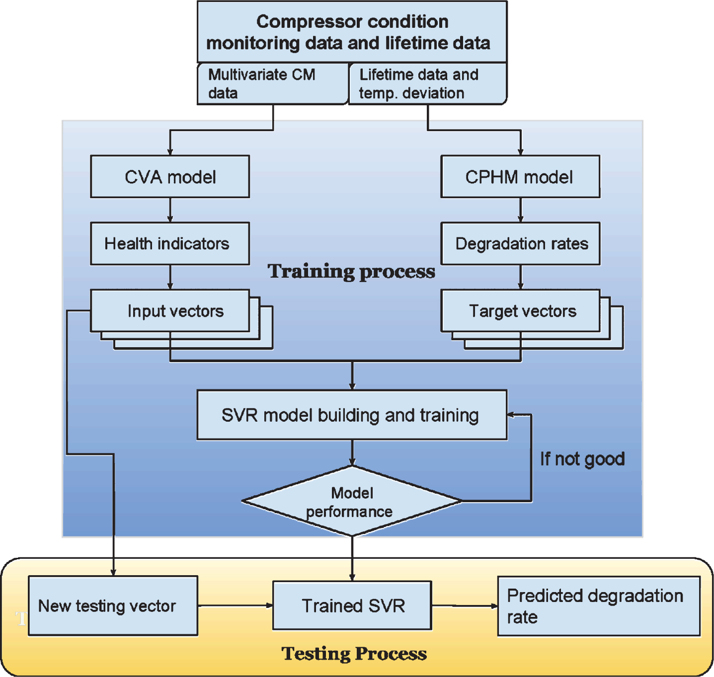
Schematic diagram of the proposed prognostic method.

3 Validation using reciprocating compressor condition monitoring data

3.1 Data acquisition

Reciprocating compressors are widely used in oil and gas industry for gas transport, lift and injection. They typically operate under high rotating speed, high pressure and high load conditions, and are therefore subject to performance degradations. These machines are highly automated with various sensors being mounted all over the system, and signals from different sensors can be stored and accessed through an e-maintenance system. The data used in this study were gathered from a two-stage, four-cylinder, double-acting reciprocating compressor used in a refinery in Europe.

The compressor experienced twelve valve failures at cylinder 4 from July 2013 to December 2014. Machine inspections revealed that the failure mode under study was valve leakage caused by broken valve plate. The failed valves were either the head end or the crank end discharge valve. A total of 12 fault cases were obtained from the site engineer and each sample was a multivariate time series consisting of 39 variables. The sampling rate was 1 Hz and the failure degradation duration for each sample was different.

3.2 CVA-based contributions for faulty variable identification

Once a fault occurs in industrial heavy-duty compressors, it is important to identify which components are most likely associated with the root-cause of the malfunction. Contribution plot analysis [4] is one of the most popular tool for identifying “fault related” variables in multidimensional statistical analysis. In this section, CVA-based state space and residual space contributions were used to identify candidate faulty variables for the compressor under study. The contributions of different process variables in fault case 3 were depicted in Fig. 2 using color map with variable number being the vertical axis and sampling time being the horizontal axis. As stated previously, the root cause of the fault was discharge valve failure in cylinder 4, meaning that the most fault related variables were variable 17 and 18 (highlighted in bold in Table 1). As shown in Fig. 2, the residual space 2-D map indicates high contributions of both variable 17 and 18 during the early stage of fault case 3. Then the contribution of variable 18 dropped to a lower level after around the 1500th sampling point, whereas variable 17 continued to show high contributions until the end of the sampling period. By looking closely at the trends of variable 17 and 18 (see Fig. 3), it was found that with the compressor controller applied to the system, variable 18 stabilized to its normal operating range after about the 1500th sample. However, due to the malfunction of HE discharge valve in cylinder 4, large deviations from normal operating conditions were observed in variable 17 until the end of the sampling period. Therefore, variable 17 rather than variable 18 was considered as a candidate faulty variable in this case.

Fig.2

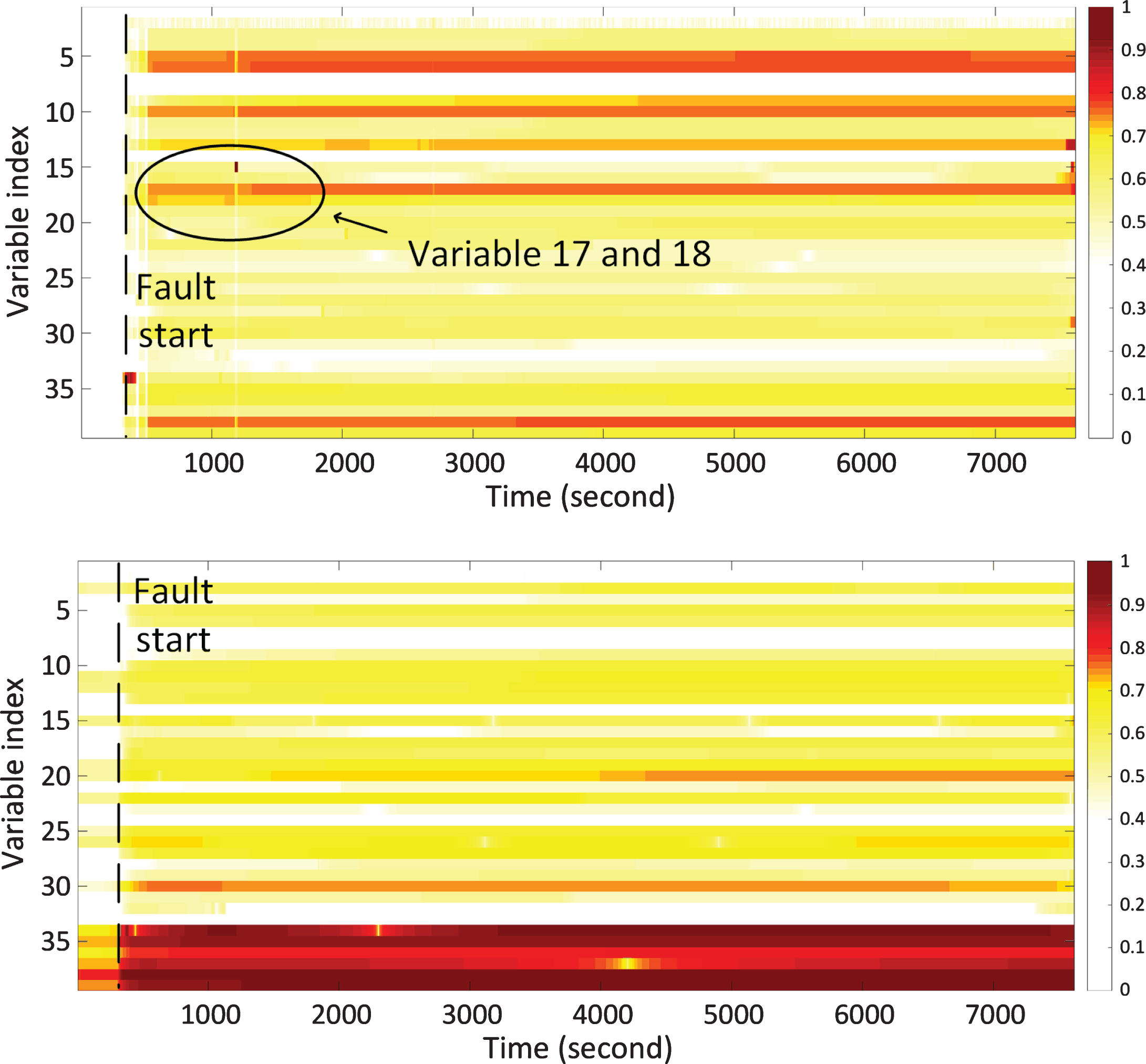
CVA-based contribution plots for faulty variable identification in fault case 3: (1) faulty variables identified in residual space (upper); (2) faulty variables identified in state space (lower). Contributions are normalized to a range of 0 to 1.

Fig.3

Trends of the HE and CE discharge valve temperature in cylinder 4 for fault case 3.

Table 1

Identified candidate faulty variables for all fault cases.

It is worth noting that in addition to variable 17 and 18, several other faulty variables were revealed by the residual and state space contributions. The reason these variables have large contributions is that the fault has propagated from cylinder 4 into other components, resulting in loss of performance of the entire compressor.

The identified candidate faulty variables for all fault cases are summarized in Table 1. Collectively, CVA-based contributions are very effective at identifying the root cause of the compressor fault as the CE/HE discharge valve temperature in cylinder 4 has been successfully reported as a faulty variable in most cases. Collectively the identified candidate faulty variables would provide valuable information to a site engineer as to the fundamental cause of the fault. In addition, it was found that the root cause was more often linked to faulty variables identified in the residual space rather than in the state space. This demonstrates the necessity of combining residual and state space contributions for fault identification as utilizing merely the state space information can lead to wrong decision making.

3.3 Determination of fault start time fault end time

Since the failure mode under study is head end/crank end valve damage took place in cylinder 4, the method employed to determine the fault start and end time, as suggested by the site engineers, is to look at the difference between crank end (CE) discharge temperature and head end (HE) discharge temperature in cylinder 4. To be specific, during healthy operating conditions and after the failure point, as shown in Fig. 4, the temperature difference between CE and HE is relatively constant. However, the temperature difference grows continuously once the valve fault occurs.

As shown in Fig. 4, the fault start time for fault case 2 was identified when the value of temperature difference starts to increase, whereas the fault end time was identified when the temperature difference stabilized at its new steady state value. The degradation duration for all failure cases can be found in Table 2.

Fig.4

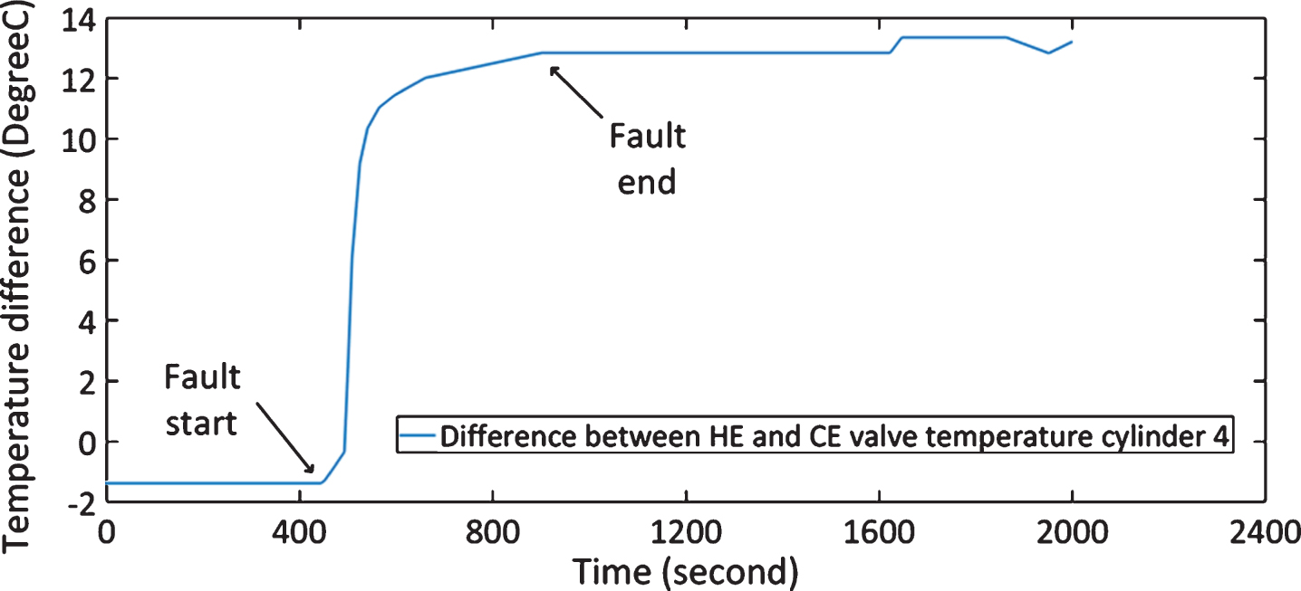
Difference between CE and HE discharge temperature in cylinder 4 – failure sample No. 2.

Table 2

Degradation duration for all failure cases

Sample No.	Degradation Length (s)
6	171
11	191
3	231
1	371
13	381
10	391
5	401
8	441
2	451
4	501
12	601
9	641

3.4 CVA model building

A CVA model was firstly built in order to transform the multivariate condition monitoring data into a one-dimensional health indicator. This process can be considered as a data fusion and dimensionality reduction procedure as it incorporates the information from all the measured 39 variables to generate a health indicator which can reflect the health condition of the system. For each fault case, a normal operating dataset was used to train the CVA algorithm to obtain the normal operating limits of $T_{t}^{2}$ , and a deteriorating dataset was used to construct a health indicator.

In order to build a CVA model as described in Equations (1 to 7), three tuning parameters need to be determined, namely, the number of time lags p and f, and the number of dimensions retained r According to the literature [17], the number of time lags p and f were determined by calculating the autocorrelation function of the root summed squares of all variables against a confidence bound of±5%. The autocorrelation function indicates how long the measured time series is correlated with itself, and thus can be used to determine the maximum number of significant lags. As shown in Fig. 5, the sample autocorrelation analysis of the training data demonstrates that the maximum number of significant lags was 25. Therefore, the number of time lags p and f were set to 25 in this study.

Fig.5

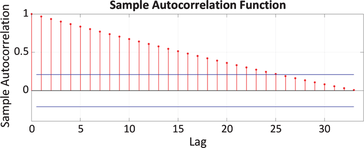
Autocorrelation of the root summed squares of all variables in training dataset.

In order to determine the optimal number of r, CVA was implemented to perform fault detection for all 12 fault cases using different values of r. The false alarm rate versus the number of retained states for all fault cases were depicted in Fig. 6. False alarm rate in this study was calculated by dividing the number of false detections by the length of the testing dataset. Then the calculated false alarm rates were averaged with the purpose of selecting the optimal value of r that minimizes the false alarm rate for all fault cases. r = 3 was finally adopted according to the results shown in Fig. 7.

Fig.6

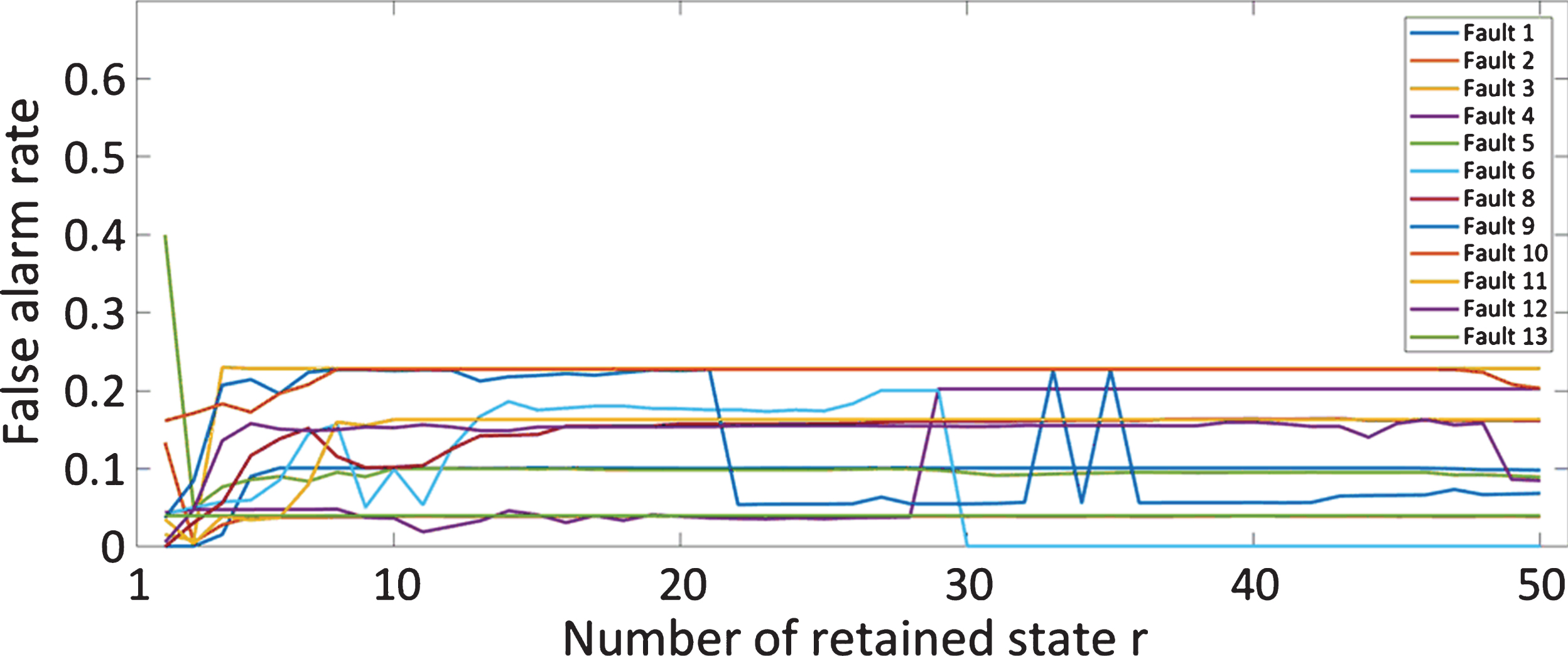
False alarm rate of all fault cases with different values of r.

Fig.7

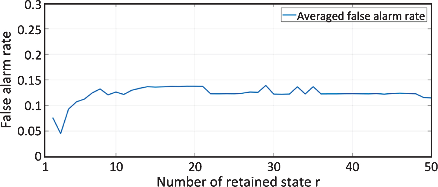
Averaged false alarm rate with different values of r.

As discussed previously, the fault start and end times in this study were determined by looking at the difference between CE and HE discharge temperature in cylinder 4. The health indicators generated by the trained CVA model were further truncated according to the fault duration of specific fault cases. Figure 8 depicts the truncated health indicators for all 12 failure cases. They will be used hereafter as target vectors for SVR training.

Fig.8

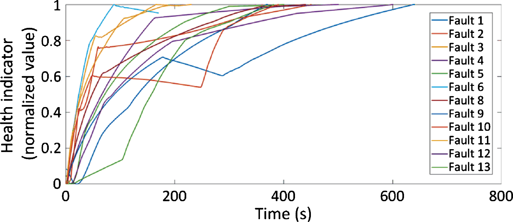
Truncated health indicators of all fault cases.

3.5 CPHM model building

In order to build a CPHM model, lifetime data of 12 fault cases were used to estimate the baseline hazard function. In addition, the difference between CE and HE discharge temperature in cylinder 4 was assumed as a covariate and the regression parameter β_k was calculated as per Equations (12 and 13) for each failure case. For example, Fig. 9 shows the calculated degradation rate of fault case 9.

Fig.9

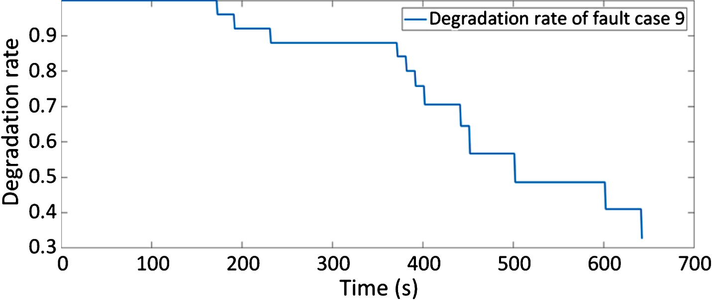
Hazard rate of failure sample no. 9.

3.6 SVR model building and testing

In this section, health indicators and failure rate vectors obtained previously were used to train a SVR model. Then the trained SVR was employed as a prognostic method to predict the failure degradation of individual failure case. To build a SVR model, we utilized a Radial Basis Function (RBF) kernel function to map input vectors into the high-dimensional feature space. The RBF kernel parameter γ and the soft margin parameter C were determined using grid search [28] together with 5-fold cross validation. For grid search, parameter γ and C take the following values:

The health indicator and degradation rate vector of fault case no. 10 were firstly utilized to train a SVR model. The optimal parameters determined by grid search were 1024 and 64 for γ and C, respectively. They were determined by searching for the minimum Root-Mean-Squared Error (RMSE) between the actual degradation rate and the estimated degradation rate for each combination of γ and C candidates (as shown in Fig. 10). Moreover, the health indicator of fault case no. 13 was used as an input vector to test the performance of the trained SVR model. The predicted degradation rate of fault no. 13 is depicted in Fig. 11. It can be observed that the predicted failure time is 381 s. 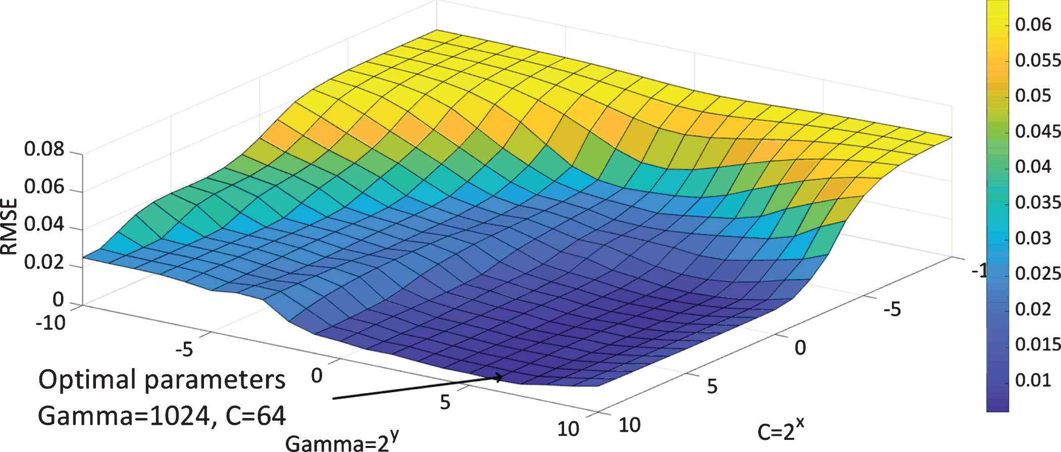$\begin{matrix} γ & = & 2^{{- 10, - 9, - 8, \dots, 10}} \\ C & = & 2^{{- 10, - 9, - 8, \dots, 10}} \end{matrix}$

Fig.10

RMSE for various values of γ and C model parameters.

Fig.11

SVR prediction for fault case no. 13.

In order to fully capture the dynamics of the compressor, a SVR model was further trained by 8 fault cases (F1, F13, F10, F5, F8, F4 and F12). The input vectors used to perform the training were obtained using the CVA method. In addition, the target vectors were acquired by an estimation of the degradation rate by means of CPHM. The optimal value of γ and C was 128 and 256 respectively according to the results of grid search. Figure 12 depicts the RMSE between the actual and the estimated target vectors for each combination of γ and C candidates. The trained SVR model was utilized to predict the hazard rate of fault case no. 2, and the predicted result is shown in Fig. 13. The predicted failure time is 449 s while the actual failure happens at 452 s.

Fig.12

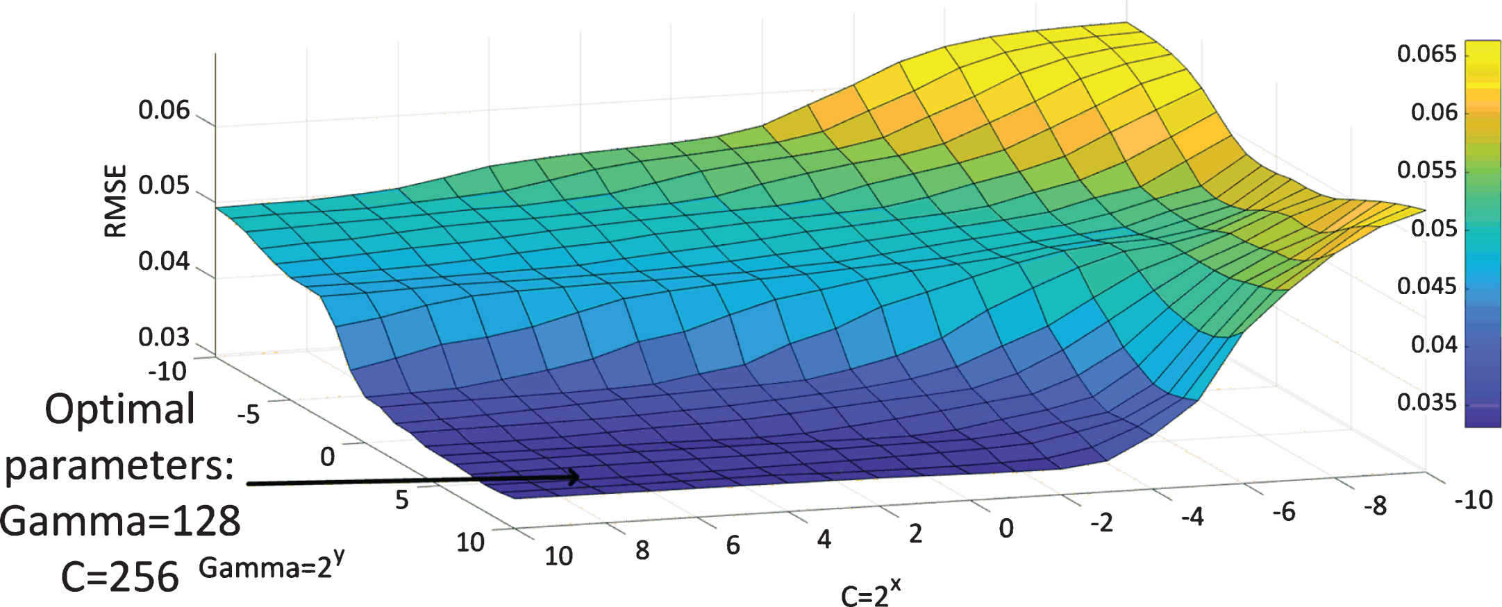
RMSE for various values of γ and C model parameters (using f1, f13, f10, f5, f8, f4, and f12 for training).

Fig.13

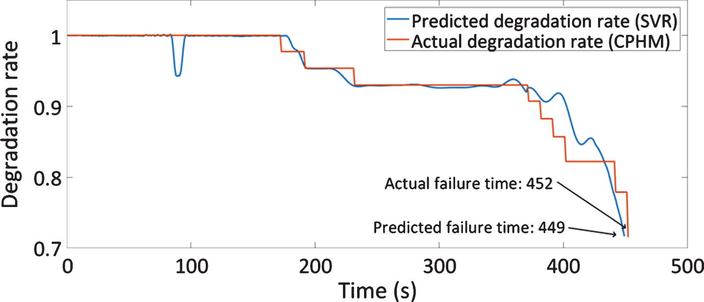
Predicted failure rate of sample no. 2.

The performance of the prognostic model can be assessed using the following metrics, namely Accuracy, root mean squared error (RMSE), mean absolute error (MAE) and Pearson’s correlation coefficient (R). Formulae of the above metrics are listed as follows: $Accuracy = (1 - \frac{T_{actual} - T_{predicted}}{T_{actual}}) \times 100 %$ (18) $RMSE = {[\sum_{i = 1}^{N} {(S {(t)}_{actual, i} - S {(t)}_{predicted, i})}^{2} / N]}^{1 / 2}$ (19) $MAE = \frac{1}{N} \sum_{i = 1}^{N} | S {(t)}_{actual, i} - S {(t)}_{predicted, i} |$ (20) $R = \frac{\sum_{i = 1}^{N} (S {(t)}_{act, i} - \bar{S {(t)}_{act}}) (S {(t)}_{pre, i} - \bar{S {(t)}_{pre}})}{\sqrt{\sum_{i = 1}^{N} {(S {(t)}_{act, i} - \bar{S {(t)}_{act}})}^{2}} \sqrt{\sum_{i = 1}^{N} {(S {(t)}_{pre, i} - \bar{S {(t)}_{pre}})}^{2}}}$ (21)

A higher value of Accuracy indicates a better the prediction. Meanwhile, the higher the value of RMSE/MAE is, the lower the prediction accuracy is. A high Pearson’s correlation coefficient means a high accordance between the actual and predicted degradation rate. The performance of the predictive model, based on the proposed four metrics, is summarized in Table 3. The predicted degradation rate of fault case no. 2 seems overestimated between 370 s and 430 s and underestimated between 431 s to 449 s, yielding a relatively high MAE value. But the accuracy is 99.33%, which is admissible for constructing the prognostic model.

Table 3

Model performance based on four statistical indexes

Sample No.	Accuracy	RMSE	MAE	R
13	99.74%	0.02	0.0082	0.9485
2	99.33%	0.0076	0.0482	0.933

4 Conclusion

In this study, condition monitoring data acquired from an operational industrial reciprocating compressor have been used to test the capabilities of CVA for fault identification. In addition, CVA combined with CPHM and SVR were applied for the first time to perform prognostics based on condition monitoring and lifetime data. 2-D contribution plots based on the variations in the residual and state spaces were utilized to identify candidate faulty variables for compressor faults. It was found that the fundamental causes are more likely to be related to the residual space. Furthermore, CPHM was utilized to calculate the fault degradation rate based on lifetime data obtained from the compressor, and the calculated degradation vectors were regarded as the target vectors for training a SVR model. Grid search and 5-fold cross validation were used to determine the optimal SVR model parameters during the training process. Finally, the trained SVR was employed to predict degradation rate and failure time of the compressor. Four metrics were utilized to evaluate the accuracy of the proposed scheme. The results illustrate that the prognostic performances were satisfied.

Although, the results of this study clearly show the superior performance of the proposed methods for fault identification and failure prediction, some aspects require further investigation are listed as follows. Firstly, apart from CE/HE discharge valve temperature in cylinder 4, several other faulty variables were reported by both the residual and state space contributions. A consideration for future work is to alleviate the smearing effect and reduce the number of reported faulty variables, thereby allowing for more accurate fault identification. Secondly, due to the approximative nature of hazard function, the degradation vectors used in this investigation are stair functions with jumps at failure times. Thus, a degradation curve might not truly reflect the deterioration process when the number of historical failures is small, which would lead to inaccurate failure time prediction. Hence, techniques should be developed to calculate machine degradation rates accurately regardless of the scarcity of lifetime data.

References

Hyvärinen

, Karhunen

, Oja

Independent Component AnalysisWiley, New York2004.

Jardine

A.K.S.

, Banjevic

, Wiseman

, Buck

and Joseph

, Optimizing a mine haul truck wheel motors’ condition monitoring program use of proportional hazards modeling, Journal of Quality in Maintenance Engineering7 (2001), 286–302.

Jardine

A.K.S.

, Anderson

P.M.

and Mann

D.S.

, Application of the Weibull proportional hazards model to aircraft and marine engine failure data, Quality and Reliability Engineering International3 (1987), 77–82.

Jiang

B.B.

, Huang

D.X.

, Zhu

X.X.

, Yang

and Braatz

R.D.

, Canonical variate analysis-based contributions for fault identification, Journal of Process Control26 (2015), 17–25.

Zupan

, Demsar

, Kattan

M.W.

, Beck

J.R.

and Bratko

, Machine learning for survival analysis: A case study on recurrence of prostate cancer, Artificial Intelligence in Medicine20 (2000), 59–75.

Guerra

C.J.

and Kolodziej

J.R.

, A data-driven approach for condition monitoring of reciprocating compressor valves, Journal of Engineering for Gas Turbines and Power136 (2014), 041601.

Cárcel

C.R.

, Cao

and Mba

, A benchmark of canonical variate analysis for fault detection and diagnosis, UKACC International Conference on Control (CONTROL), IEEELoughborough, UK, 2014, pp. 425–431.

Cox

D.R.

, Regression models and life-tables, Break throughs in StatisticsSringer, New York, 1992, pp. 527–541.

Russell

E.L.

, Chiang

L.H.

and Braatz

R.D.

, Fault detection in industrial processes using canonical variate analysis and dynamic principal component analysis, Chemometrics and Intelligent Laboratory Systems51 (2000), 81–93.

10.

Harrou

, Nounou

M.N.

, Nounou

H.N.

and Madakyaru

, Statistical fault detection using PCA-based GLR hypothesis testing, Journal of Loss Prevention in the Process Industries26 (2013), 129–139.

11.

Serdio

, Lughofer

, Pichler

, Buchegger

, Pichler

and Efendic

, Fault detection in multi-sensor networks based onmultivariate time-series models and orthogonal transformations, Information Fusion20 (2014), 272–291.

12.

, Qin

S.J.

and Yuan

, Data-driven root cause diagnosis of faults in process industries, Chemometrics and Intelligent Laboratory Systems159 (2016), 1–11.

13.

Stefatos

and Hamza

A.B.

, Dynamic independent component analysis approach for fault detection and diagnosis, Expert Systems with Applications37 (2010), 8606–8617.

14.

Hotelling

, Relations between two sets of variates, Biometrika28 (1936), 321–377.

15.

Jackson

J.E.

, Quality control methods for several related variables, Technometrics1 (1959), 359–377.

16.

Huang

L.Z.

, Cao

Y.P.

, Tian

X.M.

and Deng

X.G.

, A nonlinear quality-relevant process monitoring method with kernel input-output canonical variate analysis, IFAC-PapersOnLine48 (2015), 611–616.

17.

Odiowei

P.-E.P.

and Cao

, Nonlinear dynamic process monitoring using canonical variate analysis and kernel density estimations, IEEE Transactions on Industrial Informatics6 (2010), 36–45.

18.

Samuel

R.T.

and Cao

, Kernel canonical variate analysis for nonlinear dynamic process monitoring, IFAC-PapersOnLine48 (2015), 605–610.

19.

Stubbs

, Zhang

and Morris

, Fault detection in dynamic processes using a simplified monitoring-specific CVA state space modelling approach, Computers & Chemical Engineering41 (2012), 77–87.

20.

Yin

, Zhu

X.P.

and Kaynak

, Improved PLS focused on key-performance-indicator-related fault diagnosis, IEEE Transactions on Industrial Electronics62 (2015), 1651–1658.

21.

Kruger

and Dimitriadis

, Diagnosis of process faults in chemical systems using a local partial least squares approach, AIChE Journal54 (2008), 2581–2596.

22.

Tran

V.T.

, AlThobiani

and Ball

, An approach to fault diagnosisof reciprocating compressor valves using Teager– Kaiser energyoperator and deep belief networks, Expert Systems withApplications41 (2014), 4113–4122.

23.

Caesarendra

, Widodo

, Thom

P.H.

, Yang

B.-S.

and Setiawan

J.D.

, Combined probability approach and indirect data-driven method for bearing degradation prognostics, IEEE Transactions on Reliability60 (2011), 14–20.

24.

W.H.

and Qin

S.J.

, Consistent dynamic PCA based on errors-in-variables subspace identification, Journal of Process Control11 (2001), 661–678.

25.

X.C.

, Duan

, Mba

and Bennett

, Multidimensional prognostics for rotating machinery: A review, Advances in Mechanical Engineering9 (2017), 1687814016685004.

26.

Zhu

X.X.

and Braatz

R.D.

, Two-dimensional contribution map for fault identification [Focus on Education], IEEE Control Systems34 (2014), 72–77.

27.

Qian

and Yan

, Remaining useful life prediction of rolling bearings using an enhanced particle filter, IEEE Transactions on Instrumentation and Measurement64 (2015), 2696–2707.

28.

Liu

Z.L.

, Zuo

M.J.

and Xu

H.B.

, Parameter selection for Gaussian radial basis function in support vector machine classification, International Conference on Quality, Reliability, Risk, Maintenance, and Safety Engineering,IEEE, Chengdu, China2012 pp. 576–581.