Daily PM 10 concentration forecasting based on multiscale fusion support vector regression

Abstract

Air is regarded as one of a fundamental element for the survival of human and other living creatures. Daily PM₁₀ concentration forecasting is a useful measure that is applied to the prevention and control of work in advance. This paper proposes a multiscale fusion support vector regression (MFSVR) method for forecasting daily PM₁₀ concentration. The method uses stationary wavelet transform (SWT) to decompose original time series of daily PM₁₀ concentration into different scales, of which the information represents wavelet coefficients of PM₁₀ concentration. At each scale, wavelet coefficients are used for training a support vector regression (SVR) model. The estimated coefficients of the SVR outputs for all of the scales applied to the reconstruction of the prediction result by the inverse SWT. To enhance forecasting of the MFSVR, a feature fusion approach that bases on partial least squares is adopted to extract the original features and reduce dimensions for input variables of the SVR model. The experimental confirmation of the proposed method is tested by applying the data of four monitoring stations between 1/1/2015 and 26/12/2015 in Lanzhou, China. The results indicate that the MFSVR approach can precisely forecast daily PM₁₀ concentration on the basis of mean absolute error, mean absolute percentage error, root mean square error and correlation coefficient criteria. This method shows a potential prospect that can be implemented in air quality prediction systems in other areas.

Keywords

multiscale stationary wavelet transform partial least squares support vector regression

1 Introduction

Poor air quality has triggered a widespread public concern, especially in densely populated urban areas, since air pollution is closely associated with the health of residents. The dominant pollutant is the particulate matter with aerodynamic diameter less than 10μm (PM₁₀) in dust-haze pollution. The primary sources of PM₁₀ are industrial emission, traffic, infrastructure construction, and other similar sources [1, 2]. These particles are particularly detrimental as they reduce not only atmospheric visibility but also cause grave human health problems through inhalation [3, 4]. In reality, several regulations have been put in place to set limits on the emissions of PM₁₀ with the aim of improving and maintaining ambient air quality standards. It is great of importance for a reliable and precise approach for forecasting PM₁₀ concentration to obey these limits because it can provide advanced PM₁₀ pollution information at least one day in advance so that people can take timely and effective emission reduction actions.

An enormous amount of the air quality numerical methods, which aim to simulate the dynamics of environmental processes on air, have been applied to forecast daily PM₁₀ concentration [5 –7]. However, these models are unsuitable in most cities because they require adequate data from diverse pollution sources, the real emission components, the detailed account of physical processes in the planetary boundary layer, as well as the main chemical reactions from exhaust gases. Owing to these external challenges, statistical methods have been universally employed as an alternative to forecasting daily PM₁₀ concentration. For instance, many linear or nonlinear regression approaches for PM₁₀ prediction have also been published [8 –10]. Nonetheless, the forecasting precision of these traditional models remains low when data are less and fluctuation.

After taking the nonlinear features of the real PM₁₀ concentration into consideration, certain approaches with nonlinear mapping function have been established. One of such, artificial neural network (ANN) has been developed and successfully used for predicting PM₁₀ concentration [11, 12]. The studies [13, 14] showed that the ANN models display better performance than the traditional statistical methods. As of late, various network structures have been designed for the ANN models [15]. In addition to, machine learning approaches have been quite excellent, and hence extensively implemented in PM₁₀ concentration forecasting. Muñoz et al. [16] conducted a contrastive work between support vector machine (SVM) and ANN to forecast PM₁₀ concentration. The SVM model exhibits better fitting capability. Wang et al. [17] predicted the daily PM₁₀ using the SVM model. Hove et al. [18] used the successive over relaxation SVM (SOR-SVM) to forecast hourly PM₁₀ concentration in urban areas. Arampongsanuwat and Meesad [19] adopted SVM optimized by particle swarm optimization algorithm for predicting PM₁₀ time series. García et al. [20] forecasted the peaks of PM₁₀ concentration by employing a k-nearest-neighbour, back propagation multilayer neural network, Bayesian classifier, and the support vector regression (SVR) machine, respectively. The comparison results thus showed that the SVR model has the best prediction performance in these approaches.

Lanzhou (102°35^′58^′^′-104°34^′29^′^′E, 35°34^′20^′^′-37°07^′07^′^′N), located in the semi-arid area of northwest China, is the capital of Gansu Province. Lanzhou urban district is a typical valley basin topography, resulting in a weak atmospheric dispersion capability [21, 22]. Various types of heavy industries (e.g., petroleum, chemistry, machinery, and metallurgy) were scattered throughout in this region [23]. These factors made it a prime zone for massive air pollution, and a top PM₁₀ polluted city in China [24]. In fact, the real PM₁₀ time series is a nonlinear dynamic system [25] and makes forecasting the PM₁₀ concentration a difficult task. A considerable amount of historical data, including PM₁₀ concentration and meteorological parameters, played important roles and helped make up for this defect. However, superior prediction abilities of the models rely on data representation, because different representations can entangle and conceal the different explanatory factors of variation behind the data [26]. Also, the multicollinearity between the independent variables can make it difficult to determine exactly the most important contributor to a physical process [27]. Consequently, feature extraction, fusion, learning, and analysis of historical data are crucial to ensure prediction precision.

This paper aims to examine the feasibility of using multiscale fusion support vector regress (MFSVR) to forecast daily PM₁₀ concentration in Lanzhou. The nonlinear mapping capability of the least squares SVR (LSSVR), the multi-resolution characteristics of wavelet transform (WT), and the multicollinearity feature fusion of partial least squares (PLS) combined to obtain higher precision. First, the daily PM₁₀ concentration was decomposed into different scales with stationary wavelet transform (SWT). Second, a PM₁₀ prediction model of wavelet coefficients was constructed with LSSVR at each scale. As the final forecast, the consequences wavelet coefficients at each sequence were reconstructed based on the inverse stationary wavelet transform (ISWT). Lastly, to support the aforesaid forecasting procedure, the original features of the daily PM₁₀ time series and the meteorological factors were analyzed to ascertain the input variables of LSSVR using PLS. Thus, the precision of the enhanced method were more suitable for practical applications.

2 Materials and methods

2.1 PM₁₀ concentration and meteorological data

Four air quality automatic monitoring stations (marked by A, B, C, D in Fig. 1) have been built in Lanzhou by the Ministry of Environmental Protection of the People’s Republic of China. The stations are part of a national network that implements regular measurements of criteria air pollutants and radiates the entire urban area of Lanzhou. The daily mean concentration data of PM₁₀ (360 samples each, totaling 4×360 samples) from four stations during 1/1/2015 to 26/12/2015 were collected from the Information Sharing Platform of Environmental Monitoring of China. Also, the meteorological data, comprising mean temperature (°C), mean atmospheric pressure (kPa), vapor pressure (hPa), relative humidity (%), precipitation (mm), wind speed (m/s), and sunshine duration (h), were obtained from the China Meteorological Data Sharing Service System.

Fig.1

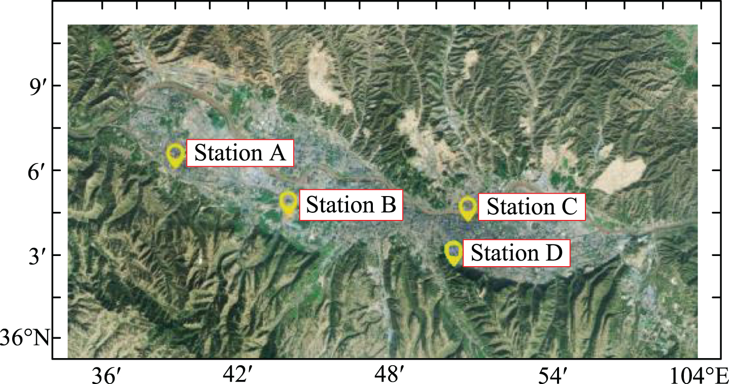
Locations of air quality automatic monitoring stations in Lanzhou urban area.

2.2 LSSVR modeling

LSSVR, a classic regression algorithm in machine learning field, is an improved version of support vector regression [28]. With the switching of inequality constraints to equality constraints in SVR, the least squares linear system takes the place of the original quadratic programming problem.

Suppose S is a training set for the daily PM₁₀ concentration forecasting, as described below $S = {(x_{i}, y_{i}), x_{i} \in R^{n}, y_{i} \in R}_{i = 1}^{l},$ (1) where x_i is i input data, y_i is a forecast value matching x_i, l is the size of training sample, and n, as model order. The LSSVR forecasting model can be expressed space as $y = ω^{T} φ (x) + b,$ (2) where φ (.) denotes the nonlinear kernel function, ω is the weight vector, and b is a bias coefficient. Under this theory, the objective function is set up ${\begin{matrix} min J (ω, ξ) = \frac{1}{2} ω^{T} ω + \frac{γ}{2} \sum_{i = 1}^{l} ξ_{i}^{2} \\ s . t . y_{i} = ω^{T} φ (x_{i}) + b + ξ_{i} \end{matrix}$ (3) where ξ represents random error between the estimated values and the true values, and γ is a regularization parameter. After Lagrange function is presented to solve this equation

$\begin{matrix} L (ω, b, ξ, α) \\ = J (ω, ξ) - \sum_{i = 1}^{l} α_{i} [ω^{T} φ (x_{i}) + b + ξ_{i} - y_{i}] \end{matrix}$ (4) where α_i is Lagrange multiplier. As the KKT optimality conditions, the solution of Equation (4) can be solved by sequential calculation

$\begin{matrix} \frac{\partial L}{\partial ω} = 0 \Rightarrow ω = \sum_{i = 1}^{l} α_{i} φ (x_{i}), \\ \frac{\partial L}{\partial b} \Rightarrow \sum_{i = 1}^{l} α_{i} = 0, \\ \frac{\partial L}{\partial ξ_{i}} = 0 \Rightarrow γ ξ_{i} - α_{i} = 0, \\ \frac{\partial L}{\partial α_{i}} = 0 \Rightarrow ω^{T} φ (x_{i}) + b + ξ_{i} - y_{i} = 0, \end{matrix}$ (5) and Equation (5) are expressed as a matrix $[\begin{matrix} 0 & q^{T} \\ q & Ω + γ^{- 1} I \end{matrix}] [\begin{matrix} b \\ α \end{matrix}] = [\begin{matrix} 0 \\ y \end{matrix}],$ (6) where q and I represent the identity matrix, Ω_ij = φ(X_i)^Tφ(X_j) = k(X_i, X_j) (j = i) represents the kernel matrix. Therefore, regarding Mercer’s condition [29], the kernel function can be written as $k (x_{i}, x) = φ (x_{i})^{T} φ (x) .$ (7)

The solutions of a and b can be gotten from Equations (6 and 7) by using the least squares method. After introducing radial basis function (RBF) kernel function [30] that is given by

$\begin{matrix} y & = & \sum_{i = 1}^{l} α_{i} k (x, x_{i}) + b \\ = & \sum_{i = 1}^{l} α_{i} exp [- \frac{{∥ x - x_{i} ∥}^{2}}{2 σ^{2}}] + b, \end{matrix}$ (8) where σ² represents the Kernel width.

Here, just two LSSVR model parameters (γ and σ²) are required to be determined. At the moment, a ten-fold cross-validation (10-CV) [31] has been used to test the precision of the model and to gain a stable model structure. Consequently, this paper selects the 10-CV to obtain the optimal γ and σ² of the LSSVR model for the PM₁₀ concentration forecasts.

2.3 Multiscale analysis

As a result of the complex changes of the nonstationary and nonlinear series, it is hard to forecast with a single scale model [32]. Multiscale analysis is an excellent tool used to extract a local information of different resolutions, thereby, providing the possibility of revealing more fully the properties of the time series [33]. In this subsection, SWT is used for decomposing the daily PM₁₀ concentration into different scales and employ the SVR model to forecast the PM₁₀ at each sequence. The multiscale SVR outputs are applied to reconstruction the final forecasting result via ISWT.

In contrast to the classical wavelet transform, e.g., discrete wavelet transform (DWT), SWT has translation invariance [34]. Using the SWT approach, the daily PM₁₀ concentration series X with a length N, the first step is to divide X into two coefficients: the approximation coefficients CA₁, is obtained by low-pass filter ${\tilde{H}}_{j}$ convolution, and the detail coefficients CD₁, gained by high-pass filter ${\tilde{G}}_{j}$ convolution. Keep in mind that the actual lengths of CA₁ and CD₁ are N rather than N/2. The second step of the process is to divide CA₁ into two parts (CA₂ and CD₂) in a similar style. The rest part of the procedure can be divided in the same manner. However, unlike DWT, SWT does not require a down-sampling operation for the transform coefficients of the approximation, as well as the detail when wavelet coefficients are decomposed. Therefore, the length is nevertheless still equivalent to that of the original time series without information loss, that is to say, SWT can realize the accurate reconfiguration of the signal [35]. The decomposition and reconstruction processes of SWT are presented in Fig. 2.

Fig.2

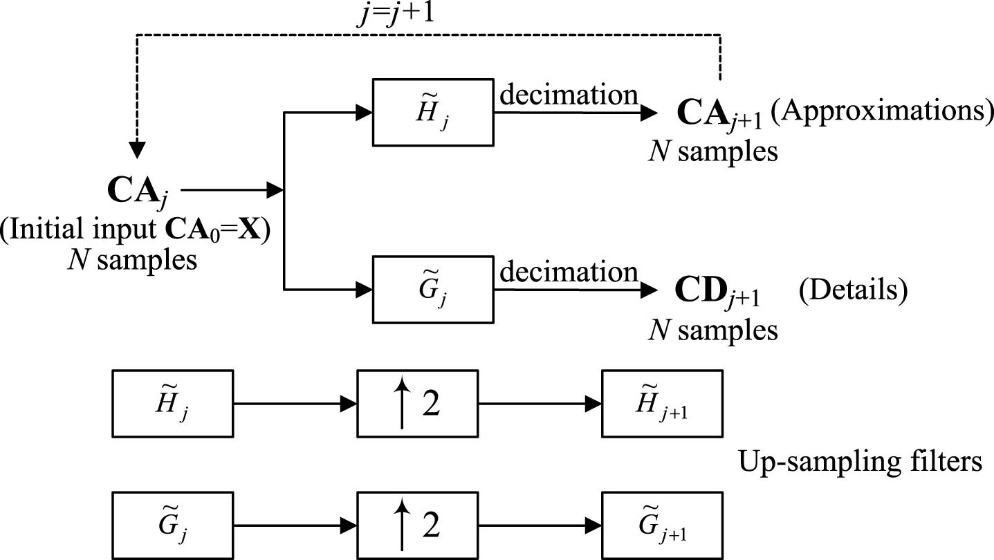
Sketch diagram of SWT decomposition and reconstruction.

As illustrated above, the original signal X is decomposed into j-level detail coefficients CD₁, CD₂, …, CD_j, and 1-level approximation coefficients CA_j with the decomposition of SWT. As a result, one gets the decomposed signals on each level in the original resolution. For the m-level (m≤j) forecasting value Y_m, its LSSVR forecasting expression is as follows $Y_{m} = \sum_{i = j + 1}^{l} α_{i, m} k (x_{m}, x_{i, m}) + b_{m} .$ (9)

As Y_m is the m-level wavelet coefficients of Y, ISWT is finally used to reconfigure Y using all levels of Y_m, that is $Y = ISWT (Y_{1}, Y_{2}, \dots, Y_{m}, \dots Y_{j}, Y_{j + 1},) .$ (10)

The multiscale SVR model for daily PM₁₀ concentration forecasting has been established. Nevertheless, what should be focused on is to simplify the computation in a practical application by fusion the original features and selecting the optimal factor. Accordingly, the feature variables of the model should be extracted in the first place. In the subsequent subsection, the PLS approach as a term refers to the connection between the dependent variables and predictor variables, used to define the input structure of the multiscale SVR model.

2.4 Feature fusion with PLS

In the 1980s, Word et al. proposed PLS [36]. PLS constructs a linear model to explain the connection between dependent variables Y and predictor variables X. This linear technique attempts to seek out the multidimensional direction in the X space which explains the maximum multidimensional covariance direction in the Y space. As a supervised feature fusion approach, PLS can rapidly and efficiently discover a low-dimensional subspace. It also has a better dimensionality reduction performance than the traditional unsupervised methods (e.g., principal component analysis).

As stated by the principle of feature fusion, the matrix X (l × n) and Y (l × 1) can be regarded as an n-dimensional predictor variable and single dependent one, respectively. Thus, the PLS model tries to search for a linear decomposition of X and Y such that $X = {TP}^{T} + E, Y = {UQ}^{T} + F,$ (11) where T_l×r is X-scores, P_n×r is X-loadings, U_l×r is Y-scores, Q_1×r is Y-loadings, E_l×n and F_l×1 are residuals. Decomposition is concluded to maximize covariance between T and U. Multiple algorithms follow a cyclic process to extract the X-scores and Y-scores. In this work, Y is a one-dimension matrix, and all possible X components will be extracted.

The extracted X-scores is a linear combination of X, like the first extracted t of X is of the form t = Xw and the initial extracted u of Y is of the form u = Yc. The extracted t and u components possess the strongest explanatory power on the variable and can carry a lot of information as feasible. Remember that w and c are the corresponding eigenvectors to the largest eigenvalue of X^TYY^TX and Y^TXX^TY, respectively. In case the first component has been extracted, the original values of X and Y would be deflated as $X_{1} = X - {tt}^{T}, Y_{1} = Y - {uu}^{T} .$ (12)

Similarly, the second component can be extracted by a new cycle. This method persists till every possible latent components t and u have been extracted. Lastly, the number of primary components needs to be determined accurately in the PLS approach. In this paper, the 10-CV was adopted to get the optimal principal components.

2.5 Overview of the MFSVR method

Based on the aforementioned explanations, Fig. 3 illustrates the flowchart for the MFSVR method used for forecasting daily PM₁₀ concentration, which is also summarized below.

Fig.3

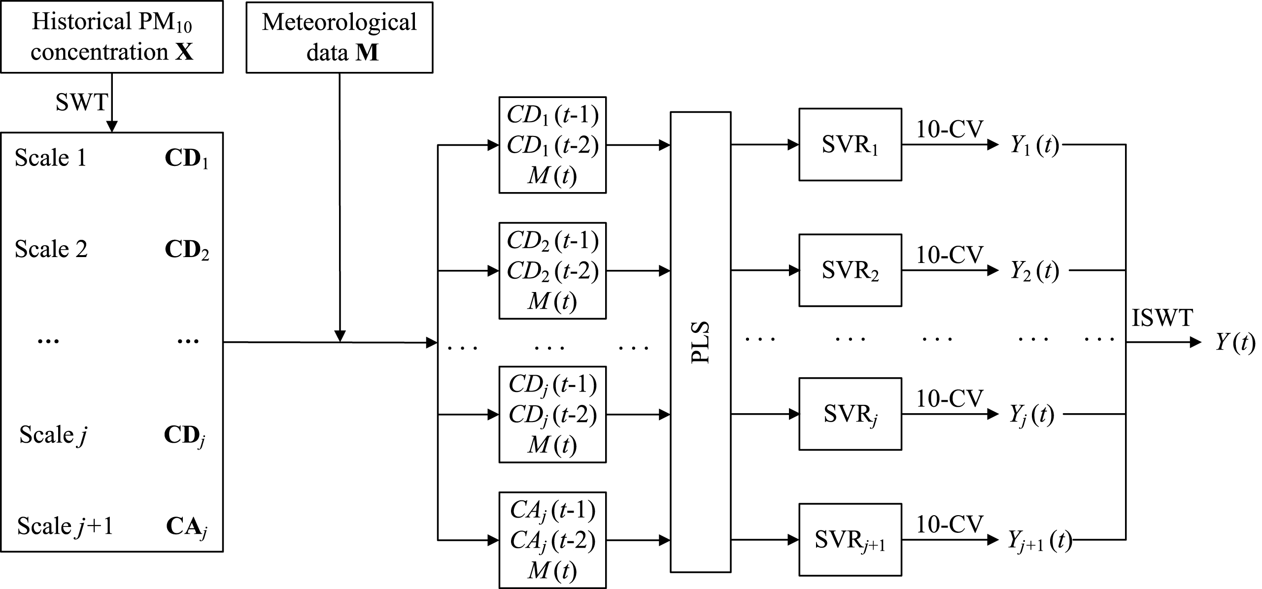
Structure of MFSVR for forecasting PM₁₀ concentration.

Step 1. Gather the modeling data of historical PM₁₀ concentration X and meteorological M.

Step 2. Execute SWT to decompose the time series X into j + 1 levels (j-level detail coefficients [CD₁, CD₂, …, CD_j] and 1-leve approximation coefficients CA_j).

Step 3. Fuse the wavelet coefficients on each level for SVR input using PLS with the (t-1)-th wavelet coefficients, the (t-2)-th wavelet coefficients and the t-th meteorological data.

Step 4. In the m-th level (m ∈ [1, j + 1]), train the SVR model utilizing the 10-CV optimized parameter γ and σ². The trained SVR model is applied to calculate the model output Y_m.

Step 5. Perform ISWT to generate the daily PM₁₀ concentration Y being calculated by Equation (10).

Step 6. Output the forecasting result. End.

2.6 Performance criteria

Multiple performance measurements can be used to assess the ability of the model in the forecasting process [37, 38]. In this study, the prediction performance and precision for PM₁₀ forecasting model are evaluated using the following criteria.

The mean absolute error (MAE) $MAE = \frac{1}{N} \sum_{t = 1}^{N} | X_{t} - Y_{t} |,$ (13)

The mean absolute percentage error (MAPE) $MAPE = \frac{100}{N} \sum_{t = 1}^{N} | \frac{X_{t} - Y_{t}}{Y_{t}} |,$ (14)

The root mean square error (RMSE) $RMSE = \sqrt{\frac{1}{N} \sum_{t = 1}^{N} {(X_{t} - Y_{t})}^{2}},$ (15)

The correlation coefficient (R²) $R^{2} = \frac{\sum_{t = 1}^{N} (X_{(t)} - \bar{X}) (Y_{(t)} - \bar{Y})}{\sqrt{\sum_{t = 1}^{N} (X_{(t)} - \bar{X})^{2} \sum_{t = 1}^{N} (Y_{(t)} - \bar{Y})^{2}}},$ (16) where N is the length of the time series, X₍t) and Y₍t) represent the values of the recorded and the forecasted, $\bar{X}$ and $\bar{Y}$ are the average values of the recorded and the forecasted respectively.

3 Results and discussion

The comparisons were made on different data sets from the four monitoring stations to examine the effectiveness of the MFSVR system and to know whether the proposed MFSVR method is superior in the elementary SVR approaches. Amongst the 360-day patterns, the first 300 daily data (1/1/2015-27/10/2015) were applied as the training set, and the rest data (28/10/2015-26/12/2015) were utilized for the test. These models were designed and ran with software Matlab 7.1.

3.1 Data description

The Fig. 4 presents the daily average PM₁₀ time series for one chosen monitoring station in Lanzhou city. There is quite an important variety of PM₁₀ concentration on a daily basis. In the mean value of 122.16μg/m³, the standard deviation of the recorded values was equivalent to 57.85μg/m³. The high values of the standard deviation affirmed the complexity of the forecasting problem. Moreover, in terms of China’s national ambient air quality secondary standards (PM₁₀ is 150μg/m³), the average daily limit of the PM₁₀ concentration is frequently exceeded, the number of days (80) exceeding the value, and the results maximum, 450μg/m³, which is particularly shocking. The results clearly illustrate that the PM₁₀ concentration maintains a high level in Lanzhou urban area all through the year. In addition, the correlation analysis approach, a term refers to the significance of a relationship between two or more variables, is used to verify the relationship between PM₁₀ concentration and weather conditions. Correlation analysis outcomes (Table 1) demonstrate that the PM₁₀ of four stations and all of the meteorological factors have a high mutual correlation (absolute value >0.1). According to the analyses above, the focus of atmospheric control work is the prevention of PM₁₀ pollution.

Fig.4

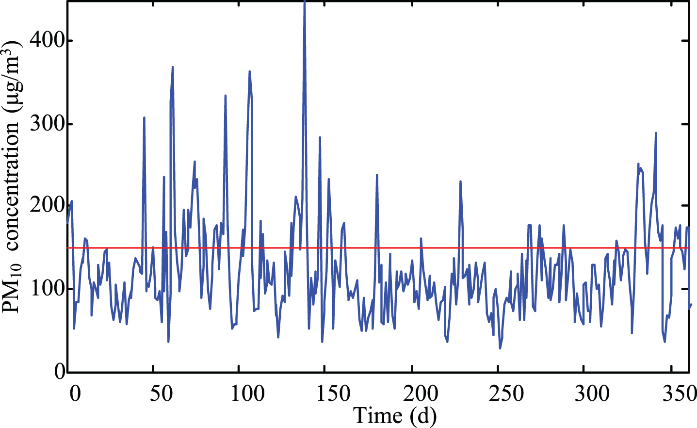
The daily averaged values of PM₁₀ concentration for the period 1/1/2015-26/12/2015 at station B in Lanzhou, China.

Table 1

Correlation analysis of daily meteorological factors and PM₁₀ concentration for Lanzhou

	T	AP	VP	RH	P	WS	I	PM₁₀
T	1.000	–0.569	–0.809	–0.021	0.178	0.051	0.184	–0.227/–0.138/–0.170/–0.113
AP		1.000	–0.468	0.097	–0.054	–0.150	–0.098	–1.133/–0.156/–0.143/–0.166
VP			1.000	0.484	0.343	–0.153	–0.085	–0.362/–0.300/–0.339/–0.272
RH				1.000	0.323	–0.340	–0.370	–0.292/–0.314/–0.344/–0.295
P					1.000	0.032	–0.193	–0.237/–0.203/–0.230/–0.202
WS						1.000	0.012	0.159/0.192/0.187/0.172
I							1.000	0.104/0.155/0.151/0.168
PM₁₀								1.000

Note: T represents mean temperature, AP represents mean atmospheric pressure, VP represents mean vapor pressure, RH represents relative humidity, P represents precipitation, WS represents mean wind speed, I represents illumination and PM₁₀ represents PM₁₀ concentration of four monitoring stations respectively. The correlation coefficients of meteorological factors and PM₁₀ are separated by the slash (/).

3.2 Specification of multiscale fusion

For SVR inputs, the original PM₁₀ time series and the weather conditions are analyzed using multiscale feature fusion with the hybrid model.

Choosing a logical wavelet function in the wavelet analysis is the first thing to consider. Normally, it is essential to select the mother wavelet function with compact support of time-frequency domain and orthogonality conditions [39]. Furthermore, the optimal decomposition scale of the PM₁₀ time series in SWT performs a crucial role in reducing the distortion and preserving the information in the data sets [40]. The number of decomposition scales controls PM₁₀ approximation in the data. In this case, the Daubechies wavelets db1 [41] is chosen as the mother wavelet in the decomposition.

Figure 5 shows the results of the 3-level wavelet decompositions of PM₁₀ at each station. All signals, from the first (CD₁) to the third (CD₃) levels and the coarse approximation CA₃ are illustrated in the original resolution. While observing the signals on different levels, one can perceive the marked difference in variability in which CA₃ is the low-frequency coefficient that maintains the shape of the original time series, and also reflects the long-term trend of PM₁₀ concentration. CD₁, CD₂, and CD₃, instead, are the high-frequency coefficient that hides the details of the original time series, and reflects the random fluctuation characteristics of the diverse focal length of PM₁₀ concentration. With this, this work can substitute the prediction task of the original series of high variability in forecasting its lower variability wavelet coefficients on different levels and utilizing Equation (10) to finalize PM₁₀ forecast at any time point. Owing to most of the wavelet coefficients are of lower variability, the increase in the whole prediction precision will be expected.

Fig.5

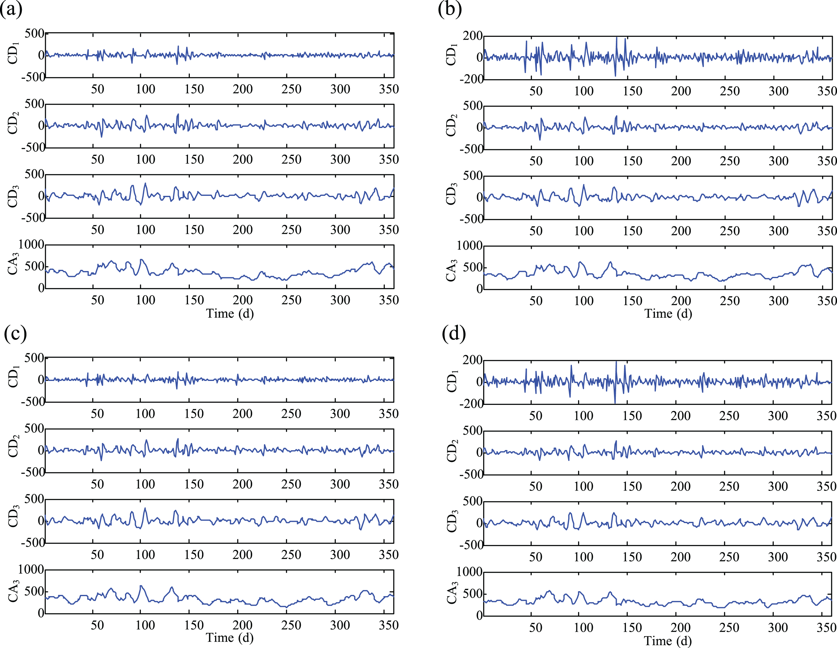
The wavelet decomposition of the recorded time series X corresponding to the PM₁₀ concentration from 1/1/2015 to 26/12/2015 at (a) Station A, (b) Station B, (c) Station C, and (d) Station D. CD₁ to CD₃ represent the detailed coefficients and CA₃ is the coarse approximation of X on three level.

The PLS method is used to overcome the multicollinearity problem in this study. There was a fuse of main information including nine predictor variables that are the wavelet coefficients in the previous two days and the total meteorological factors of the day. As stated in Section 2.4, the optimum amount of principal components are found by 10-CV. Looking at the studies above, Table 2 gives the PLS process results at diffident scales. It can be seen that PLS is performed to fuse the first few principal components and their cumulative variance explained in X are more than 98% of the factors. Subsequently, a few principal components are utilized to replace the forecaster variables X as the input data of the SVR model at each sale. However, it is to be noted that the cumulative variance explained in Y convey significant variances on different levels. It can prove that the weather conditions and historical PM₁₀ data have a complex effects on the current PM₁₀ pollution in multiple scales. Thus, it is a successful procedure to expose intrinsic regularity of the PM₁₀ concentration.

Table 2

PLS analysis of the factors for the MFSVR model

Factors	PC	CVE_X (%)	CVE_Y (%)
CD₁
Station A	4	98.55	12.43
Station B	4	98.46	12.59
Station C	4	98.98	13.75
Station D	4	98.63	13.26
CD₂
Station A	3	98.16	55.42
Station B	4	99.69	57.06
Station C	4	99.75	55.00
Station D	4	99.65	54.56
CD₃
Station A	3	98.73	73.57
Station B	3	98.75	74.78
Station C	3	98.73	74.16
Station D	3	98.42	73.51
CA₃
Station A	2	98.41	95.06
Station B	3	99.26	94.22
Station C	2	98.04	93.82
Station D	3	99.07	93.07

Note: PC represents the number principal components, CVE_X represents cumulative variance explained in X, and CVE_Y represents cumulative variance explained in Y.

3.3 Forecast evaluation and model comparison

As mentioned above, the optimum model inputs on each level of the MFSVR model consisting of four monitoring stations are concluded in Table 2. Moreover, the optimal structure parameters γ and σ² of MFSVR are gained by 10-CV. Based on Table 2, the wavelet coefficients of each scale can be forecasted, and then the final result is reconstructed using ISWT. To evaluate the dominance of the proposed method, SVR and fusion support vector regression (FSVR) are also applied to forecast the daily PM₁₀ concentration. This FSVR is a term that is a hybrid model using combination of SVR as predictor and PLS as a data fusion tool.

Figure 6 presents the prediction results for these three models of four monitoring stations, respectively. To measure the dispersal between the recorded value and the forecast results, the box plots of absolute errors were also shown in Fig. 6, explaining the lower error between the two data sets.

Fig.6

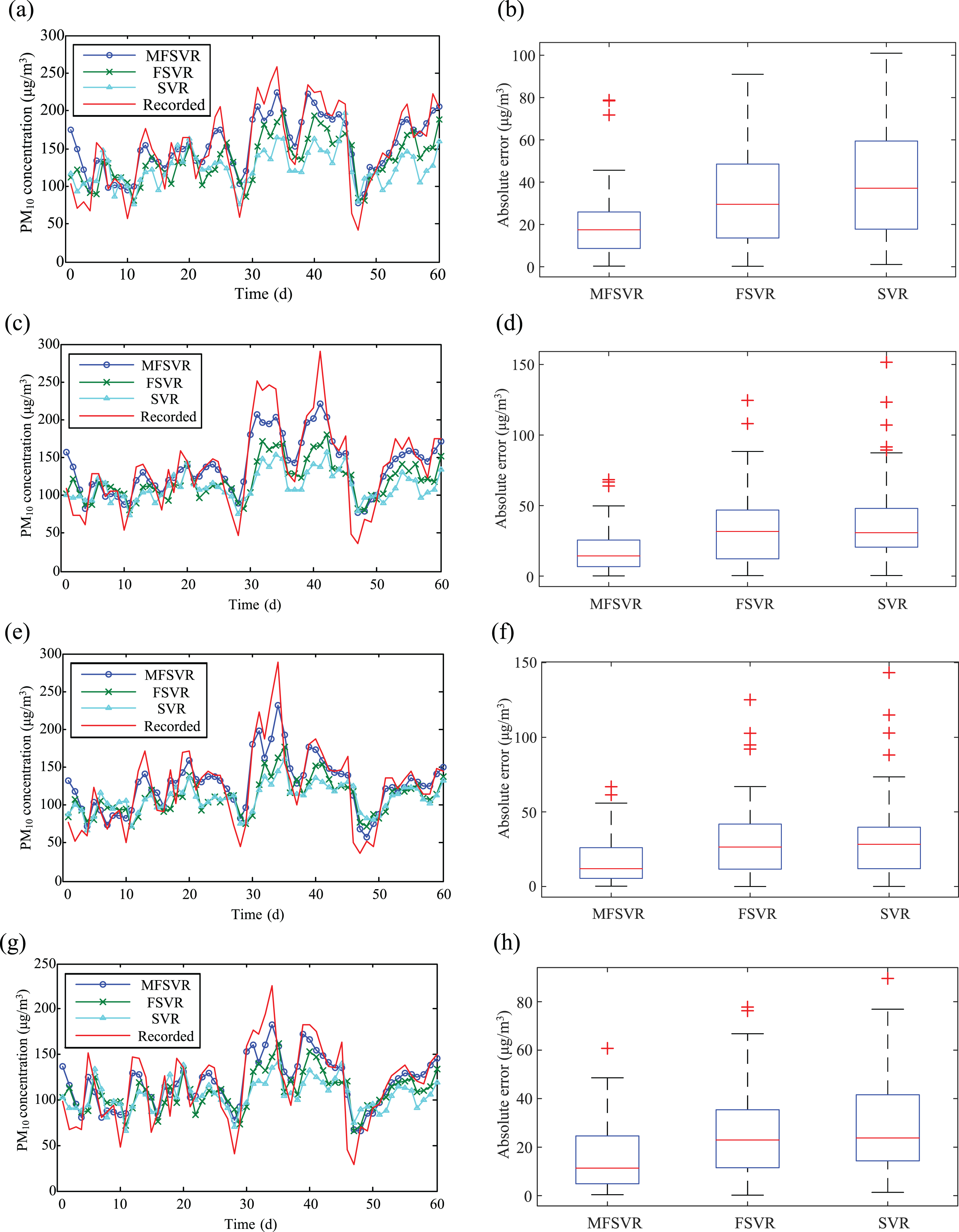
Forecasting results (left) and box plots of absolute errors (right) using different models at (a and b) Station A, (c and d) Station B, (e and f) Station C, and (g and h) Station D.

As seen in Fig. 6, the forecasting results of the proposed model are nearer to the recorded values compared to the values generated by SVR and FSVR in four monitoring stations. Apart from a few extreme points, it is able to follow the changes in the testing data accurately, and the forecasted values are consistent with the recorded ones. The box plots show that the distributions of the absolute error for the MFSVR model are the most concentrated, followed by FSVR and SVR. Furthermore, the position of the entity for the proposed model is lower compared to the two other models. Most errors of the proposed approach is thus within a lower range. Hence, when using SVR only, it is clear that the prediction performance of the testing data is inadequate indicating that it is hard to get a good result in a single model.

Based on illustrations discussed above, the proposed MFSVR approach shows obvious superiority in the PM₁₀ concentration prediction. Moreover, the Friedman test [42], a classical nonparametric test method, is applied to further analyse if there is a statistically significant difference between MFSVR, FSVR and SVR for each one of the four monitoring stations. In this work, under the null hypothesis (H₀): the independent, prediction model, is assumed to have no effect on the dependent, the value of absolute error; the three models have the same prediction error.

The formula of the Friedman test is $Q = \frac{12}{CK (K + 1)} \sum_{I = 1}^{K} R_{I}^{2} - 3 C (K + 1),$ (17) where C means the number of days to predict PM₁₀ concentration, K represents the number of forecasting models for each monitoring station, and R_I is the sum of ranks in each model. The numbers 12 and 3 are constants, not rely on the number of models or experimental conditions. The test statistic Q is distributed according to the standard normal distribution with K - 1 degrees of freedom when the null hypothesis is true, i.e. when the independent variable is having no effect on the dependent variable.

Take station B, for example, each model’s absolute errors are ranked and the ranked errors in each column are summed (R_I). Values of absolute error from Fig. 6(d) are substituted into Equation (17) to calculate the Q equals 17.5, and the critical value of normal distribution with two degrees of freedom for P is equivalent to 0.000 (P≤0.05). Thus, one reject H₀: and conclude that the absolute errors were significantly different in the three models. In addition to, Friedman test are performed with the three other monitoring stations, and the P values are equal to zero. The results show that there is significant difference between the three models at each monitoring station, as reflected in the size of the absolute error. The test results in Table 3 (e.g., R_I of station B for MFSVR, FSVR, and SVR are 94.8, 124.8, and 139.8, respectively) also prove that the most suitable performance is the MFSVR model for forecasting PM₁₀ concentration, the second is FSVR, SVR is the worst.

Table 3

Friedman test results of absolute error valuables using different models at each monitoring station

Model	C	Median	R _I
MFSVR	60	17.5/14.3/11.9/11.3	90.0/94.8/91.2/88.8
FSVR	60	29.6/31.6/26.5/23.0	127.8/124.8/127.2/133.2
SVR	60	37.1/30.8/28.3/23.8	142.2/139.8/142.2/138.0

The wavelet analysis, which has excellent time-frequency characteristics and multi-resolution capability, is proficient in extracting the internal regularity of the PM₁₀ series by transforming it into different scales. Likewise, the dimension from the unqualified variables and noises feature fusion can be reduced by feature fusion of the input data. Thus, the proposed MFSVR method can elevate the appropriate degree of complex features in multiscale and finally achieve an improved forecasting performance.

Besides, a quantitative assessment is implemented. Table 4 presents the prediction performances applying the MFSVR, the FSVR and the SVR model, respectively. It shows that the forecasting effect of the developed method is far enhanced than that of the corresponding FSVR and SVR in all four criteria.

Table 4

Comparison of the forecasting performances of different models

Stations	Model	Performance criteria
		MAE (μg/m³)	MAPE (%)	RMSE (μg/m³)	R²
A	MFSVR	19.99	18.64	26.35	0.89
	FSVR	33.68	25.45	40.99	0.72
	SVR	39.77	27.10	47.64	0.71
B	MFSVR	19.49	19.73	25.64	0.92
	FSVR	33.73	27.93	42.94	0.76
	SVR	38.78	29.54	49.12	0.73
C	MFSVR	17.62	20.20	23.82	0.91
	FSVR	31.13	28.93	40.75	0.67
	SVR	32.81	30.24	42.99	0.65
D	MFSVR	16.12	19.45	21.09	0.89
	FSVR	26.49	27.51	32.73	0.66
	SVR	28.56	27.99	34.82	0.65

According to Table 4, take station B for example, when compared with SVR, MAE, MAPE and RMSE of FSVR are lower than 5.01μg/m³, 1.61%, and 6.16μg/m³, respectively, while R² is higher than 0.03. This is due to the PLS approach can use features information to eliminate the multicollinearity in the SVR model. Moreover, the hybrid FSVR model improves training speed and grid search. It can be seen that the whole computation time that is marked is saved. Also, it was seen that MAE, MAPE, and RMSE of MFSVR decreased by 42.23%, 29.36%, 40.29% respectively while R² of MFSVR rose by 21.05% when contrasted with those of FSVR. The mono-SVR method has a good forecasting precision in the stationary phase of the time series. Nevertheless, it becomes swiftly lower during fluctuation period. This result shows that the partial sample contains a small amount of information. In other words, the multiscale characterization can explain the sophisticated internal features. Furthermore, one noticed that another three monitoring stations attain the same outcomes as the station B. This similarity also shows that the MFSVR approach has a great generalization ability in the field about air quality prediction.

Regarding the comparisons mentioned above, all the results sufficiently show that the developed method, which is combining the SVR and the multiscale fusion, demonstrates the best forecasting effect compared to the other methods.

4 Conclusions

The forecasting approach to the daily PM₁₀ concentration is presented in the paper by applying multiscale fusion support vector regression. The decomposition of mixed features time series into several different subsequences with multiple simple features and by employing the use of prediction strategy for each of them at several scales is one extraordinary innovation of this approach. The application of this approach has divided the forecasting issue into a few more uncomplicated tasks to enhance the prediction precision. Another innovation of this method is using feature fusion as a new input at each scale based on PLS. This input extracted from the wavelet coefficients of PM₁₀ concentration, and meteorological factors can replace the first collection of data. The hybrid model performs better than the single model and to some extent; it resolves oversized input dimension problems. The planned model has been tested using the data of four monitoring stations in Lanzhou, China. Also, the present method is compared with SVR and FSVR. The results indicated by executing the multiscale fusion, the MFSVR approach outperforms the two other models looking at the four criteria, hence creating the way for the optimal forecasting of air pollution system.

Footnotes

Acknowledgments

This work was supported by the Ministry of Environmental Protection of the People’s Republic of China (2111101). In addition, the authors are indebted to the editors/reviewers for their insightful comments and suggestions to help improve the quality of this paper.

References

Contini

, Genga

, Cesari

, Siciliano

, Donateo

, Boveand

M.C.

, Guascito

M.R.

, Characterisation and source apportionment of PM₁₀ in an urban background site in Lecce, Atmospheric Research95 (1) (2010), 40–54.

Salvador

, Artíñano

, Viana

M.M.

, Querol

, Alastuey

, González-Fernández

and Alonso

, Spatial andtemporal variations in PM₁₀ and PM_2.5 across Madrid metropolitan area in 1999–2008, Procedia Environmental Sciences4 (2011), 198–208.

Medina

, Plasencia

, Ballester

, Mücke

H.G.

and Schwartz

, Apheis: Public health impact of PM₁₀ in 19European citie, Journal of Epidemiology & Community Health58 (10) (2004), 831–836.

Qiu

, Yu

I.T.

, Wang

, Tian

, Tse

L.A.

, Wong

T.W.

, Differential effects of fine and coarse particles on daily emergency cardiovascular hospitalizations in Hong Kong, AtmosphericEnvironment64 (2013), 296–302.

Friberg

M.D.

, Zhai

, Holmes

H.A.

, Chanq

H.H.

, Strickland

M.J.

, Sarnat

S.E.

, Tolbert

P.E.

, Russell

A.G.

and Mulholland

J.A.

, Method for fusing observational data and chemical transport modelsimulations to estimate spatiotemporally resolved ambient airpollution, Environmental Science & Technology50 (7) (2016), 3695–3705.

Zhang

, Denero

S.P.

, Joe

D.K.

, Lee

H.H.

, Chen

S.H.

, Michalakesand

, Kleeman

M.J.

, Development of a source oriented version of the WRF/Chem model and its application to the California regional PM₁₀/PM_2.5 air quality study, Atmospheric Chemistry and Physics14 (1) (2014), 485–503.

Jeong

J.I.

, Park

R.J.

, Woo

J.H.

, Han

Y.J.

and Yi

S.M.

, Source contributions to carbonaceous aerosol concentrations in Korea, Atmospheric Environment45 (5) (2011), 1116–1125.

Ul-Saufie

A.Z.

, Yahaya

A.S.

, Ramli

N.A.

, Hamid

H.A.

, Performanceof multiple linear regression model for long-term PM₁₀concentration prediction based on gaseous and meteorological parameters, Journal of Applied Sciences12 (14) (2012), 1488–1494.

Vlachogianni

, Kassomenos

, Karppinen

, Karakitsios

and Kukkonenet

, Evaluation of a multiple regression model for theforecasting of the concentrations of NO_x, andPM₁₀, in Athens and Helsinki, Science of the Total Environment409 (8) (2011), 1559–1571.

10.

H.D.

, Lu

W.Z.

, Xue

, Prediction of PM₁₀concentrations at urban traffic intersections using semi-empiricalbox modelling with instantaneous velocity and acceleration, Atmospheric Environment43 (40) (2009), 6336–6342.

11.

Antanasijević

D.Z.

, Pocajt

V.V.

, Povrenović

D.S.

, Ristić

M.Đ

and Perić-Grujić

A.A.

, PM₁₀ emission forecasting using artificial neuralnetworks and genetic algorithm input variable optimization, Science of the Total Environment443 (15) (2013), 511–519.

12.

Bai

, Li

, Wang

, Xie

, Li

, Air pollutantsconcentrations forecasting using back propagation neural networkbased on wavelet decomposition with meteorological conditions, Atmospheric Pollution Research7 (3) (2016), 557–566.

13.

Caselli

, Trizio

, Gennaro

G.D.

and Ielpo

, A simplefeedforward neural network for the PM₁₀ forecasting:Comparison with a radial basis function network and a multivariatelinear regression model, Water Air & Soil Pollution201 (1-4) (2009), 365–377 .

14.

Şahin

Ü.A.

, Bayat

and Uçan

O.N.

, Application ofcellular neural network (CNN) to the prediction of missing airpollutant data, Atmospheric Research101 (1–2) (2011), 314–326.

15.

Singh

K.P.

, Gupta

, Kumar

, Shukla

S.P.

, Linear and nonlinearmodeling approaches for urban air quality prediction, Science of the Total Environment426 (2012), 244–255.

16.

Muñoz

, Martin

M.L.

, Turias

I.J.

, Jimenez-Come

M.J.

and Trujillo

F.J.

, Prediction of PM₁₀ and SO₂exceedances to control air pollution in the Bay of Algeciras, Spain, Stochastic Environmental Research and Risk Assessment28 (6) (2014), 1409–1420.

17.

Wang

, Liu

, Qin

, Zhang

, A novel hybrid forecastingmodel for PM₁₀ and SO₂ daily concentrations, Science of the Total Environment505 (2015), 1202–1212.

18.

Hou

, Li

, Zhang

, Xu

, Zhang

, Li

, Wei

, Ma

, Using support vector regression to predict PM₁₀and PM_2.5, 35th International Symposium onRemote Sensing of Environment (ISRSE35)17 (2014), 012268–In:.

19.

Arampongsanuwat

, Meesad

, PM₁₀ prediction model by support vector regression based on particle swarm optimization, Advanced Materials Research403-408 (2011), 3693–3698.

20.

García

E.M.

, Rodríguez

M.L.M.

, Jiménez-Come

M.J.

, Espinosa

F.T.

and Domínguez

I.T.

, Prediction of peak concentrationsof PM₁₀ in the area of Campo de Gibraltar (Spain) using classification models, Soft Computing MODELS in Industrial andEnvironmental Applications, 6th International Conference SOCO 201187 (2011), 203–212.

21.

X.Q.

, Ma

A.Q.

, Wang

H.L.

, Analyzing on air pollution spatialdistribution of Lanzhou using GIS, Arid Land Geography29 (4) (2006), 576–581.

22.

Chu

P.C.

, Chen

, Lu

, Li

, Lu

, Particulate air pollutionin Lanzhou China, Environment International34 (5) (2008), 698–713.

23.

Zhang

, Li

, Bravo

M.A.

, Jin

, Nori-Sarma

, Xu

, Guan

, Wang

, Chen

, Wang

, Tao

, Qiu

, Zhang

and Bell

M.L.

, Air quality in Lanzhou, a major industrial city in China:Characteristics of air pollution and review of existing evidence from air pollution and health studies, Water Air and SoilPollution225 (2014), 2187.

24.

Tao

, Mi

, Zhou

, Wang

, Xie

, Air pollution andhospital admissions for respiratory diseases in Lanzhou, China, Environmental Pollution185 (2014), 196–201.

25.

Dotse

S.Q.

, Dagar

, Petra

M.I.

, Silva

L.C.D.

, Influence ofSoutheast Asian Haze episodes on high PM₁₀,concentrations across Brunei Darussalam, Environmental Pollution219 (2016), 337–352.

26.

, Sanchez

R.V.

, Zurita

, Cerrada

, Cabrera

and Vásquez

R.E.

, Multimodal deep support vector classification with homologous features and its application to gearbox fault diagnosis, Neurocomputing168 (2015), 119–127.

27.

Yeganeh

, Motlagh

M.S.P.

, Rashidi

, Kamalan

, Prediction ofCO concentrations based on a hybrid partial least square and supportvector machine model, Atmospheric Environment55 (2012), 357–365.

28.

X.J.

, Cheng

Z.Q.

, Yu

Q.B.

, Bai

, Li

, Water-qualityprediction using multimodal support vector regression: Case study ofJialing River, China, Journal of Environmental Engineering143 (10) (2017), 04017070.

29.

Mercer

, Functions of positive and negative type, and theirconnection with the theory of integral equations, Philosophical Transactions of the Royal Society of London209 (1909), 415–446.

30.

Miao

, Zhang

, Liu

Z.W.

, Zhang

, Conditionmulti-classification and evaluation of system degradation processusing an improved support vector machine, Microelectronics Reliability75 (2017), 223–232.

31.

Arefi

, Clustering regression based on interval-valued fuzzyoutputs and interval-valued fuzzy parameters, Journal of Intelligent & Fuzzy Systems30 (3) (2016), 1339–1351.

32.

Bai

, Wang

, Li

, Xie

, Wang

, A multi-scale relevancevector regression approach for daily urbanwater demand forecasting, Journal of Hydrology517 (2014), 236–245.

33.

, Liang

, Time-frequency signal analysis for gear boxfault diagnosis using a generalized synchrosqueezing transform, Mechanical Systems and Signal Processing26 (2012), 205–217.

34.

Jumah

A.A.

, Denoising of an image using discrete stationary wavelet transform and various thresholding techniques, Journal ofSignal and Information Processing4 (1) (2013), 33–41.

35.

, Liang

, Separation of the vibration-induced signal of oil debris for vibration monitoring, Smart Materials and Structures20 (4) (2011), 045016.

36.

Wold

, Ruhe

, Wold

, Dunn

W.J.

, The collinearity problem inlinear regression. The partial least squares (PLS) approach togeneralized inverses, SIAM Journal on Scientific andStatistical Computing5 (3) (1984), 735–743.

37.

Chen

, Shi

, Shu

, Gao

, Ensemble and enhancedPM₁₀ concentration forecast model based on stepwiseregression and wavelet analysis, Atmospheric Environment74 (2013), 346–359.

38.

Bai

, Sun

, Zeng

, Li

, A multi-pattern deep fusion modelfor short-term bus passenger flow forecasting, Applied Soft Computing58 (2017), 669–680.

39.

Feng

, Li

, Zhu

, Hou

, Jin

, Wang

, Artificialneural networks fore casting of PM_2.5, pollution usingair mass trajectory based geographic model and wavelet transformation, Atmospheric Environment107 (2015), 118–128.

40.

Siwek

, Osowski

, Improving the accuracy of prediction ofPM₁₀, pollution by the wavelet transformation and an ensemble of neural predictors, Engineering Applications of Artificial Intelligence25 (6) (2012), 1246–1258.

41.

Rafiei

, Niknam

, Khooban

M.H.

, A novel intelligent strategyfor probabilistic electricity price forecasting: Wavelet neuralnetwork based modified dolphin optimization algorithm, Journal of Intelligent & Fuzzy Systems31 (1) (2016), 301–312.

42.

Friedman

, The use of ranks to avoid the assumption of normality implicit in the analysis of variance, Journal of the American Statistical Association32 (200) (1937), 675–701.

Daily PM 10 concentration forecasting based on multiscale fusion support vector regression

Abstract

Keywords

1 Introduction

2 Materials and methods

2.1 PM10 concentration and meteorological data

3.1 Data description

Footnotes

Acknowledgments

References

2.1 PM₁₀ concentration and meteorological data