
Abstract
Development of power through wind with the enhancement of renewable energy resources, frolics/romps a principal role in a developing country like India due to its censorious locations. Wind speed prediction in long term scenario has become a key research area in distinct applications (i.e., management of energy, optimal designing of wind farm, restructuring of electricity marketing, load-shedding and load forecasting). However, forecasting of accurate wind speed data for installation of wind turbine is very difficult due to its deterministic and probabilistic characteristics. The presented technique in this study may bridge the research gap related with the long term wind speed forecasting as resolve the previously indicated problems. Thence, two basically distinct techniques, k-nearest neighbors (kNN) algorithm and artificial neural network (ANN), have been implemented to forecasting of monthly wind speed of Indian cities. The uniqueness of the presented paper is to predict the wind speed in common form of incoming month by implementing the kNN algorithm. A dataset of current wind speed recorded specimen from 168 cities of India is utilized to train and test the proposed approach. Obtained results through the proposed approach have been validated by using ANN technique, which shows very small MSE.
Introduction
The forecasting of wind power plays an essential role in management of power by government of a country as well as for an utility. An unswerving and highly meticulous forecasting develops good planning as well as control of power like access power storage, load scheduling and transmission [1]. When forecasting of the wind power is not possible directly, then forecasting of wind speed (WS) becomes more significant, because WS is related with wind power directly. Types of Wind speed forecasting are short–term (ST), medium-term (MT) and long-term (LT) which may be utilized by power industry and/or power market for trading and management purposes. The study of ST wind speed prediction is necessary for avoiding the collapse to wind turbine due storm, whereas LT wind speed forecasting is useful for produced power planning [2].
Wind power and/or WS prediction models can be categorized into two types (i.e., statistical and physical models). In physical models, WS forecasting is performed by using meteorological datasets. Numerical approach for weather forecasting is an example of physical prediction model [3]. In the available literature, statistical models for WS and wind power forecasting are linear-time-series (LTS) based model and persistence model. ANNs model and ANFIS type models are also a part of statistical models. Persistence approach is simple whereas LTS based models are widely used model.
Whenever, forecasting is more than six hours, then LTS and physical models are not suitable due to probabilistic characteristic of wind. To overcome such problem, numerous non linear methods (i.e., ANNs and ANFIS) [4–8] are utilized for forecasting the WS as given in the literature as some are reviewed in next section [9–21].
In this paper, a comparison of kNN with state of the art ANNs model have been presented whose inputs are measured metrological datasets of 168 cities of India. The performance comparison is shown of 25 different cities and represented graphically.
Rest of paper is assembled as follows: The state-of-the-art for WS prediction using ANN models is represented in Section-2, used datasets are explained in Section-3. Methodology developed in this study has been represented in Section 4 and obtained results from the methodology have been described in detail in Section 5. Finally, summery of the work has been described in Section 6 as a conclusion.
Related work
Review of literature
Based on available online database, several researches have been done in the area of wind speed (WS) forecasting. Some of them have been explained as given below:
S. Buhan et al. have implemented a model based on statistical approach. Authors have applied both ANN and SVM model to predict WS of 25 power plant of Turkey. The mean absolute error (MAE) of the presented approach is in range of 1.5% to 5.2%. MAEs are 12.63% and 16.85% for Multistage and single stage respectively which is comparatively very high [9].
A. Kusaik and Z. Zhang represent a case study of short term WS forecasting using different AI models (i.e., ANN, SVM, Random forest, Boosting Tree) to identify the wind behaviour and a comparison is presented. The prediction accuracy 90% at 60 s time period. Out of different AI models, SVM identify WS very closer to measure value for 1 hour prediction whereas for 4 hour prediction, ANN has given good results that mean ANN is not suitable for short time WS prediction for this problem [10].
T.G. Barbounis et al. Presented a long term WS prediction model RNNN (Recurrent network neural network), and MLP. The performance indexes are measured in term of MAE and RMS [11].
S. Li et al. have designed ANN with 4 inputs for WS prediction and then wind power. Proposed method’s performance is 1% -2% but taken large time for multiple inputs [12].
Ronay Ak et al. have implemented two different hybrid models (ANN with GA and ELM with kNN) for forecast time-series WS in Canada. The prediction accuracy of NN with CP is 90% and ELM with CP is 90.6% [13].
C.S. Ioakimidis et al. have Implemented probabilistic wind power potential through WS prediction using ANN hourly though South of Portugal dataset. The prediction accuracy is approximate 75% [14] which is very poor for installation of wind turbine.
T.G Barbounis and J.B. Theocharis have designed a fuzzy based recurrent ANN. Proposed approach is utilized to identify multi step wind predictions from remote locations. Proposed model enhance the reasonable accuracy as compare with ANN and Fuzzy [15].
J. Wang et al. have developed a hybrid approach using RBF for real time WS identification of Hexi Corridor, China. The performance of the proposed approach is very low in the range of 12%–16% which is comparatively higher than existing MLP, ESM, RBFN, SAM-ESM, SAM-RBFN and ESM-RBFN. The main disadvantage of the proposed approach is to predict only hourly WS [16].
P. Ramasamy et al. have developed ANN approach for WS identification using measured dataset from western Himachal Pradesh, India. Obtained wind power through proposed approach is vary from 773.6 to 5329.8 watt, which is comparably higher [17].
H. Shao [18] conducted study on wind speed forecasting by proposing Wavelet Transformation (WT) and AdaBoosting neural networks. The data provided by state grid includes air pressure, WS, and air temperature. The AdaBoosting NN is utilized to enhance the prediction accuracy. The forecasting performance is measured by RMSE, MAE, and RMAE. The average forecasting accuracy evaluated by TRD is higher than TRA.
H. Borhan at al. [19] proposed method for WS estimation based on pattern recognition (PR) using ANNs. The proposed model uses NARX (Non Linear Autoregressive Network) 10 year wind data. The proposed method is compared with two different real dataset and has been compared with other methods. MAE is utilized as performance analyzer of the model, which shows the results that MAE is minimum with proposed scheme as comparedto others.
Findings
After critical review of literature, we found some findings related with wind speed forecasting: Datasets for training, testing and validation are chosen for ANN model based on deterministic WS. Architecture configuration (input layer neuron-hidden layer neuron-output layer neurons) is chosen for ANN model based on WS conditions. A lot of research scope is available for WS prediction (i.e, ST, MT and LT) for wind farm installation. The prediction accuracy of WS is varied with variation of input variable so exact value should be recorded for accurate prediction by ANN model. Prediction accuracy needs to be enhanced as conventional artificial intelligence techniques are not suitable for this problem. The accuracy is changed with variation of input variables, so selection of input variables are another big finding for this problem. Input variable selection to enhance the forecasting accuracy of WS.
To bridge these research gaps, kNN and ANN have been implemented in this paper for proper understanding.
Data set used
Credential datasets are collected from two different resources in this study. Dataset#1 has been collected form recorded data by CWET of 168 cities (Table 1) of distinct reasons of India [20] whereas dataset#2 has been collected from online freely available data provided by NASA [21]. Four different data files have been prepared from this dataset. Data samples in training, testing, validation and prediction files are 93, 25, 25 and 25 cities’s data sets, selected randomly. Each file is distinct to each other. Thirteen input variables are used for WS prediction in this study. Thirteen input variables (i.e., Lat.-Latitude, Long-Longitude, RH-Relative humidity, EL-Elevation, AP-Atmospheric pressure, SR-Daily solar radiation, AT-Air temperature, ET-Earth temperature, CD-Cooling degree-days, HD-Heating degree-days, CDT-Cooling design temperature, HDT-Heating design temperature and ET-Earth temperature amplitude) are utilized in this study. Dataset matrix is shown in Equations 1 to 4.
Recorded Datasets of 168 Indian cities utilized for training, testing, validation and one month ahead prediction
Recorded Datasets of 168 Indian cities utilized for training, testing, validation and one month ahead prediction
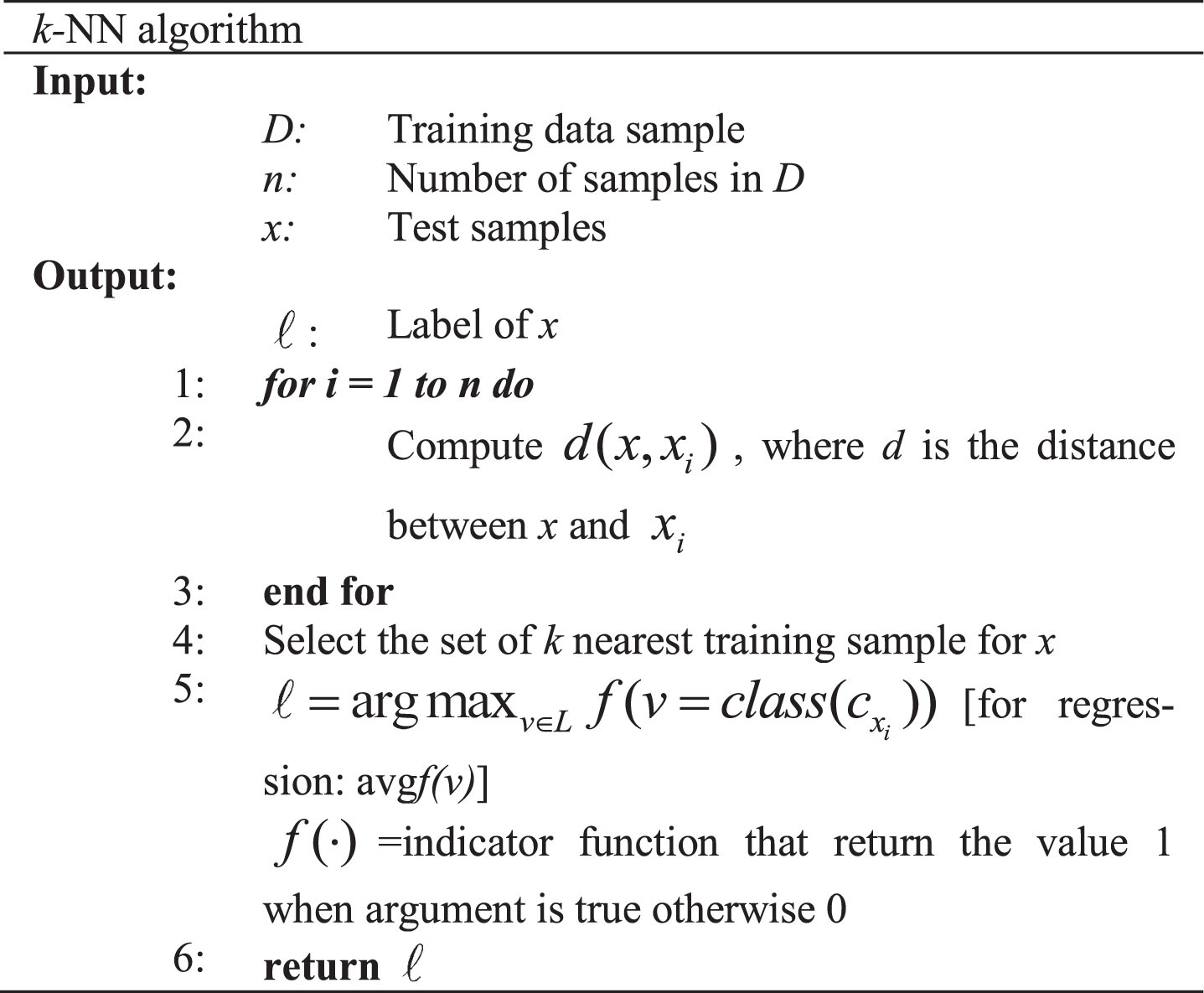
k-nearest nieghbors algorithm (k-NN) [22]
In data mining, k-NN is a non-parametric approach utilized for both regressions as well as classification purpose. In k-NN, the input includes k training samples whereas the output depends on the application of k-NN (whether use for regression or classification). For classification purpose: the output is classified by a majority vote of neighbors (i.e. assigned class corresponding to each sample) For regression purpose: the output is defined by the average of the value of its k-NNs
k-NN algorithm is a lazy type learning or instance-based learning in which function is only approximated locally and is a simplest algorithm amongst the all data mining algorithms. k-NN is also assign the weight to neighbors contribution in which nearer neighbors contribute more than other.
Lets us assume, a data set (x, y) , (x1, y1) , …, (x n , y n ), where y is the target value of the data sample x, so that x|y = r □ p r for r = 1,2 and p r = probability distribution.
In the training phase, k-NN algorithm stores the feature vectors and corresponding target level. To evaluate the distance metric for continuous variables is Euclidean distance and for discrete variables, overlap metric (or Hamming distance) is evaluated as given by Equations 5 to 8.
where,
The k-NN accuracy can be enhanced if distance metric is learned by LMNN (large margin neighbor) or by NCA (neighbourhood component analysis). A major drawback of k-NN is skewed. To overcome this problem in k-NN, the class/target value of each k nearest points (sample) is multiplied by a weight proportional to the inverse of the distance from that point to the test point.
In parameter selection: the choice of k depends upon the data. To reduce the effect of noise, larger value of k is used. When k = 1, the predicted value is closest to training sample, and can be optimized by some other techniques.
The main logic of k-NN algorithm is to evaluate a set of k objects in training data set that are closer with test data set. The basic idea of k-NN algorithm is shown as below:
There are two type of perceptron NN (i.e., Single layer perceptron (SLP) and Multilayer Perceptron-MLP). SLP is utilized for linear classification whereas for nonlinear problem MLP is used. Multilayer Perceptron were introduced by Werbos in 1974 and revised by Rumelhart, McClelland, and Hinton in 1986 which are also called feed forward networks (FFN). Usually, perceptron evaluate a discontinuous function which is represented as:
Where, m is the smoothed function which is represented as:
With
These Eq. are called logistic equation. Logistic functions have the property that they are monotonically increasing, continuous and differentiable. Multilayer Perceptron is an acyclic graph in which nodes are neurons with logistic activation. The process of MLP Training is same as training of a SLP. The weight value of two neurons in MLP is also varying to minimize the error value as given:
or
Where, tg= target value, out= model output (from j to p NN layer).
Updation of Weight between two neurons may be performed through a series of rules (w updating rules) which are represented as:
It is the only output
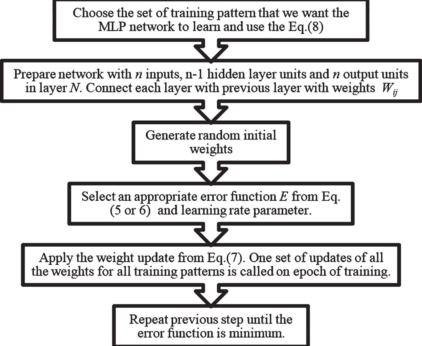
Training Multilayer Perceptron.
For implementing k-NN and MLP models data is collected from two resources: 1) NASA and 2) measured value from CWET of 168 cities of India. These datasets of 168 cities have been divided into four groups randomly. Group1 contain the dataset of 93 cities and utilized for designing and training the model. In group2, 25 cities’s dataset have been included and utilized for testing purpose of the designed and trained model. Again 25 cities dataset (group3) have been used for validation purpose of the trained and tested model. Finally, group4 contains remaining 25 cities data sets which are utilized for future forecasting purposes. These four groups dataset are totally different to each other. Training, testing, validation and prediction data includes 1116, 300, 300, and 300 samples respectively of 13 variables.
Results and discussion
Both k-NN and MLP approaches have been designed and run for training, testing and validation datasets by using MATLAB R2014a (8.3.0.532, win32/64) on a Lenovo Y700 PC. The configuration of the PC has 2.6-GHz Intel Core i7-6700HQ processor with 16GB of RAM; a 1TB, 5,400-rpm HDD with a 128GB SSD. The graphical representations of obtained result during all operating phases have been represented in Figs. 2–4 respectively. On analyzing the plots (Figs. 2–4) it has been identified that k-NN provide WS values which are very closer to recorded WS from real sites of Indian cities. For the comparison point of view, MLP method has been implemented for the same dataset, which shows that obtain results from kNN is much better than MLP. Moreover, the wind power of a location is depends upon the condition of WS of that location as represented by Equation (16). So, before installation of any wind turbine/farm, correct identification of WS is become more realistic without installation ofmetrological substation. In that scenario, kNN model will play an important roll to predict the WS in actual manner without a metrological substation. The WS forecasting accuracy through MLP method is 94.0% whereas through kNN method is 99.1%.

Training phase results.
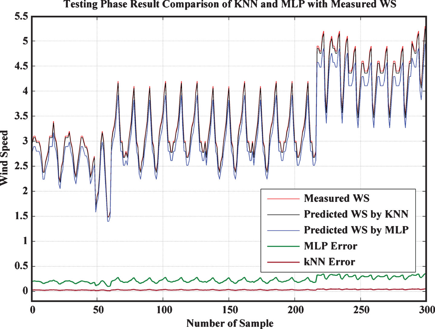
Testing Phase results.
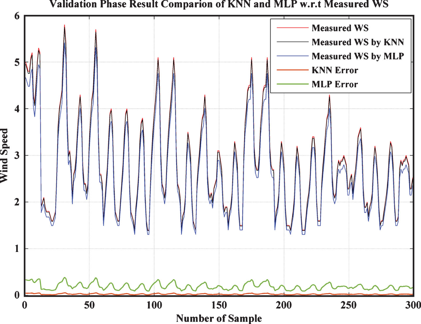
Validation Phase Results.
Figure 2 represents the training phase output as well as error variation with respect to number of samples for kNN and MLP methos. Here, red line represents the kNN performance whereas, green line for MLP performance.
The represented data samples in the training, testing and validation phase are very large. Therefore, there is not an easy task to make distinguish between measured and predicted value by the model. To overcome this problem, we have plotted again these training, testing and validation phase results by using “rose” method of plotting as shown in Fig. 5. By using this method, we can easily distinguish the predicted value and measured value of wind speed.

Angle histogram plot for a) Training phase, b) testing phase and c) validation phase.
Presented study in this paper represents the comparative study of two approaches named kNN and MLP and results obtained from these approaches are further validated by forecasting the WS for a new unknown dataset of 25 cities of Indian states. Predicted results have been compared with recorded value through the metrological station provided by CWET centre of India and graphically represented in Fig. 6.

Comparison of Predicted Wind speeds by k-NN and MLP methods of 25 cities mentioned in Table 4.
In this paper k-NN and MLP models are developed for prediction of long term wind speed (one month ahad wind speed). Data of 168 cities of India is collected from NASA as well as measured data from CWET which is used in this study. The input variables which are used in this paper are 13 (i.e., Lat., Long., RH, EL, AP, SR, AT, ET, CD, HD, CDT, HDT and ET). On comparing these two models it is found that k-NN gives better results than MLP model.
The future scope is to implement the proposed kNN approach at real site for the forecasting of WS in deterministic and probabilistic environmental conditions. Moreover, to select the most relevant input variables for WS forecasting is another future scope of this study which has been performed in coming research.