Multiple target detection and tracking on urban roads with a drone

Abstract

Recently, drone technology has developed rapidly for various purposes. A drone is very useful for aerial surveillance due to its remote sensing capability. Multiple target detection and tracking are essential to recognize any harmful threats in advance, however the image captured at a distance is easily degraded due to blurring and noise as well as low resolution. This paper addresses the detection and tracking of moving vehicles with drone imaging. A drone captures video sequences of multiple moving vehicles from a distance. Cars and buses are the objects of interests driving on urban roads. The detection step consists of frame difference followed by thresholding and morphological operation considering the size of region of interest (ROI). The centroids of the ROI’s are considered measurements for tracking. Tracking is performed with interacting multiple model (IMM) filtering, which estimate the state of vectors and covariance matrices using multiple modes of Kalman filtering. The measurements in the validation region are associated with established tracks by the nearest neighbor rule. In the experiment, total seven moving cars and buses are captured at a long distance by a drone. It will be shown that the proposed method well detects the moving vehicles and achieves a good accuracy in estimating their locations.

Keywords

Drone imaging object detection multiple target tracking IMM filtering frame difference

1 Introduction

Recently, there is increased usage of unmanned aerial vehicles (UAVs) or drones for aerial surveillance. The usage of drones is cost effective and the camera installed in the drone is easily manipulated to capture the scenes of interest. Thus, the advanced technology in drones can build efficient surveillance systems [1].

Multiple object detection and tracking is important for security and surveillance [2]. Various researches have been performed for visual detection and tracking of moving objects in the literature. Methods based on background subtraction and frame difference are studied in [3 –9]. Gaussian mixture modeling (GMM) was used to analyze background and target regions [3 –5]. Scale invariant feature transform (SIFT) was adopted to extract foreground objects from the background scene [6, 7]. In [8], background was subtracted under Gaussian mixture assumption followed by morphological filters. Long range moving objects are detected by a drone in [9]. In [10, 11], moving cars are detected with a background image and they are tracked by Kalman filtering.

Many studies have been conducted on multiple target tracking [10 –15]. High-maneuvering, closely located multiple targets, heavy clutter (false alarm), and low detection probability are often considered difficulties to overcome [12]. Kalman filtering provides a solution for estimating the state of the target in real time. It is known optimal under independent Gaussian noise assumption [13]. Interacting multi model (IMM) is actively applied to targets of high maneuvering due to its adaptation capability switching to multiple modes [14]. When multiple measurements are detected at a frame, data association is required to assign the measurements to the established tracks [12, 15].

In this paper, we address the detection and tracking of multiple moving vehicles on urban roads captured by a drone. A drone captures videos sequence of moving cars and buses from a long distance. Object detection is performed through frame difference followed by thresholding, morphological filtering, and regions of interest (ROI) size limitation. The frame difference is calculated using two frames at a constant interval. Then, thresholding is applied to generate a binary image. Two morphological operations: erosion and dilation are applied to the binary image to produce candidate ROI’s, which are disjoint alternative areas representing moving vehicles. Finally, false ROI’s are removed by comparing the size of the ROI with the real object sizes. The centroids of all ROI’s are fed to the tracking stage as measured two dimensional positions.

Tracking is performed by IMM filtering to estimate the state of the target and the covariance matrix. A nearly constant velocity (NCV) models with two difference covariance matrices of the process noise are assumed for the dynamic states of the target [14], that is, each IMM mode is set up with a different process noise. A gating process excludes the measurement outside the validation region. The nearest measurement-to-track association scheme assigns one measurement to one track [10, 11]. In the experiments, total seven moving cars or buses are captured at a long distance at a height of 100 meter by a drone. Experimental results show that their locations are well detected and tracked with good accuracy by a proposed method.

The remains of the paper are organized as follows. Object detection is discussed in Section II. Multiple target tracking is presented in Section III. Section IV demonstrates experimental results. Conclusion follows in Section V.

2 Object detection with frame difference

The block diagram of object detection is described in Fig. 1. First, the difference between the current and the past frames at a constant interval is obtained and then, a thresholding step follows to generate a binary image as

Fig.1

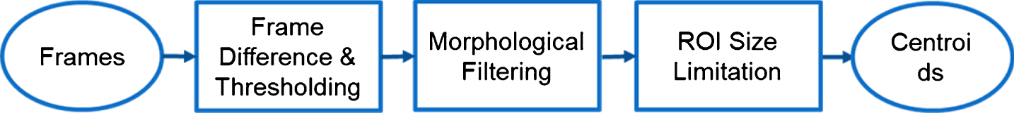
Block diagram of moving object detection.

$\begin{matrix} \begin{matrix} I_{T} (m, n; k) \\ = {\begin{matrix} 1, & if | I (m, n; k) - I (m, n; k - k_{d}) | > θ_{T} \\ 0, & otherwise \end{matrix}}, \\ m = 1, \dots, M, n = 1, \dots, N \end{matrix} \end{matrix}$ (1) where I (m, n ; k) and I_B (m, n ; k - k_d) are the k-th frame and the (k - k_d)-th frame, respectively, k_d is a constant interval for frame difference, θ_T is a thresholding value, and M and N are pixel sizes in x and y directions, respectively. Two morphological operations: erosion and dilation, are applied sequentially to the binary image to segment moving vehicles. Erosion and dilation filtering are, respectively, definedas [16] $I_{E} = {l | E_{l} \cap I_{T}^{c} = φ},$ (2) $I_{D} = {l | D_{l} \cap I_{E} \neq φ},$ (3) where E and D are the structuring elements for erosion and dilation, respectively. It is noted that E_l ={ e + l|e ∈ E } and D_l ={ d + l|d ∈ E }, where l stands for an integer value less than the image size. In the experiments, three operations (erosion, dilation, and erosion) are applied to generate candidate ROI’s. The last step is to remove false ROI’s as $O_{i} (m, n) = {\begin{matrix} 1, & θ_{S} \leq Size {O_{i}} \leq θ_{f} \\ 0, & otherwise \end{matrix}},$ (4) where O_i is the i-th ROI, θ_s and θ_f are the minimum and the maximum size of ROI. The value of θ_s and θ_f are based on the true size of car and buses, respectively, in the scene. The center of each ROI is considered a measurement for target tracking in the next section.

3 Target tracking with IMM filtering

3.1 System modeling

The dynamic state of the target is modeled as a nearly constant velocity (NCV) model; the targets’ maneuvering is modeled by the uncertainty of the process noise, which is assumed to follow the Gaussian distribution. The following is the discrete state equation of a target: $x (k + 1) = F (Δ) x (k) + q (Δ) v (k),$ (5) $F (Δ) = [\begin{matrix} 1 & Δ & 0 & 0 \\ 0 & 1 & 0 & 0 \\ 0 & 0 & 1 & Δ \\ 0 & 0 & 0 & 1 \end{matrix}], q (Δ) = [\begin{matrix} Δ^{2} / 2 & 0 \\ Δ & 0 \\ 0 & Δ^{2} / 2 \\ 0 & Δ \end{matrix}],$ (6) where $x (k) = {[\begin{matrix} x & \dot{x} & y & \dot{y} \end{matrix}]}^{T}$ is the state vector at frame k, T denotes matrix transpose, Δ is the sampling time, and v (k) is a process noise vector which is Gaussian white noise. Two modes are set up for IMM filtering with different covariance matrices of v as $Q_{1} = diag ([\begin{matrix} σ_{1 x}^{2} & σ_{1 y}^{2} \end{matrix}])$ and $Q_{2} = diag ([\begin{matrix} σ_{2 x}^{2} & σ_{2 y}^{2} \end{matrix}])$ . A measurement vector is composed of two components in x and y directions. The following is the measurement equation: $z (k) = H x (k) + w (k),$ (7) $H = [\begin{matrix} 1 & 0 & 0 & 0 \\ 0 & 0 & 1 & 0 \end{matrix}],$ (8) where w (k) is a measurement noise vector which is Gaussian white noise with the covariance matrix, $R = diag ([\begin{matrix} r_{x}^{2} & r_{y}^{2} \end{matrix}])$ .

3.2 Multi-mode interaction

The state vectors and the covariance matrices of the IMM mode filters at the previous frame k - 1 are mixed to generate the initial state vectors and the covariance matrices for each of the IMM mode filter at the current frame k. The initial state vector and the covariance matrix of target t for mode j with the mixing probabilities are obtained, respectively, as $\begin{matrix} {\hat{X}}_{0 j}^{t} (k - 1 | k - 1) \\ = \sum_{i = 1}^{r} {\hat{x}}_{i}^{t} (k - 1 | k - 1) μ_{i | j}^{t} (k - 1 | k - 1), \end{matrix}$ (9) $\begin{matrix} P_{0 j}^{t} (k - 1 | k - 1) \\ = \sum_{i = 1}^{r} {\begin{matrix} μ_{i | j}^{t} (k - 1 | k - 1) {P_{i}^{t} (k - 1 | k - 1) + \\ [{\hat{x}}_{i}^{t} (k - 1 | k - 1) - {\hat{x}}_{0 j}^{t} (k - 1 | k - 1)] \times \\ [{\hat{x}}_{i}^{t} (k - 1 | k - 1) - {\hat{x}}_{0 j}^{t} (k - 1 | k - 1)]^{T}} \end{matrix}} . \end{matrix}$ (10) $μ_{i | j}^{t} (k - 1 | k - 1) = \frac{p_{ij} μ_{i}^{t} (k - 1)}{\sum_{i = 1}^{r} p_{ij} μ_{i}^{t} (k - 1)},$ (11) $i = 1, \dots, r, j = 1, \dots, r, t = 1, \dots, N_{t},$

where r is the number of IMM filter modes, ${\hat{x}}_{i}^{t} (k - 1 | k - 1)$ and $P_{i}^{t} (k - 1 | k - 1)$ are, respectively, the state vector estimation and the covariance matrix for target t and mode i at frame k - 1, $μ_{i}^{t} (k - 1)$ is the mode probability of target t and mode i at frame k - 1, p_ij is the mode transition probability, and N_t is the number of targets.

3.3 Mode matched Kalman filtering

Kalman filtering is performed for each IMM mode. The first step is to predict the state of a target when the dynamic state is modeled by mode j [14]: ${\hat{x}}_{j}^{t} (k | k - 1) = F {\hat{x}}_{j}^{t} (k - 1 | k - 1),$ (12) $P_{j}^{t} (k | k - 1) = {FP}_{j}^{t} (k - 1 | k - 1) F^{T} + Q_{j},$ (13) where ${\hat{x}}_{j}^{t} (k | k - 1)$ and $P_{j}^{t} (k | k - 1)$ are, respectively, the state prediction and the covariance prediction for target t and mode j at frame k. Next, the residual covariance $S_{j}^{t} (k)$ and the filter gain $W_{j}^{t} (k)$ are obtained as $S_{j}^{t} (k) = {HP}_{j}^{t} (k | k - 1) H^{T} + R,$ (14) $W_{j}^{t} (k) = P_{j}^{t} (k | k - 1) H^{T} S_{j}^{t} (k)^{- 1} .$ (15)

3.4 Measurement gating and data association

Measurement gating is a pre-process of data association that reduces the number of candidate measurements. Data association is the process of associating multiple measurements to established tracks [12]. Figure 2 illustrates an example of the gating process. Each ellipsis shows the validation region of each target. Track 1 and 2 are initialized at frame 1 and 2, respectively. They intersect each other between frame 5 and 6. When no measurement exists inside the validation region of track 1 at frame 4, the state estimate is the same with the state prediction for track 1. At frame 5, two measurements are detected, but only one is associated with track 1, which is inside the validation region. Two measurements exist in the validation region of track 2, where the nearest neighbor association rule is applied to assign one measurement to the prediction of track 2.

Fig.2

Illustration of gating process and data association.

Let Z (k) be a set of m_k measurement vectors at frame k: $Z (k) = {z_{m} (k)}, m = 1, \dots, m_{k} .$ (16)

The measurement gating is performed by chi-square hypothesis testing assuming the Gaussian measurement residuals. Thus, a set of valid measurements for target t and mode j at frame k is obtained as as

$\begin{matrix} Z_{j}^{t} (k) & = & {z_{m} (k) | ν_{mj}^{t} (k)^{T} [S_{j}^{t} (k)]^{- 1} ν_{mj}^{t} (k) \leq γ, \\ m = 1, \dots, m_{j}^{t} (k)}, \end{matrix}$ (17) $ν_{mj}^{t} (k) = z_{m} (k) - H {\hat{x}}_{j}^{t} (k | k - 1),$ (18) where γ is the gating size, and $m_{j}^{t} (k)$ is the number of candidate measurements for target t and mode j at frame k. We adopt the nearest neighbor rule to associate a measurement with track t by minimizing the norm of the residual as ${\hat{m}}_{j}^{t} (k) = \underset{m = 1, \dots, m_{j}^{t} (k)}{arg min} | | ν_{mj}^{t} (k)^{T} [S_{j}^{t} (k)]^{- 1} ν_{mj}^{t} (k) | | .$ (19)

3.5 State estimate and covariance update

The state estimate and the covariance matrix of targets are updated as ${\hat{x}}_{j}^{t} (k | k) = {\hat{x}}_{j}^{t} (k | k - 1) + W_{j}^{t} (k) ν_{{\hat{m}}_{j}^{t} (k) j}^{t} (k),$ (20) $P_{j}^{t} (k | k) = P_{j}^{t} (k | k - 1) - W_{j}^{t} (k) S_{j}^{t} (k) W_{j}^{t} (k)^{T} .$ (21)

If $m_{j}^{t} (k)$ is equal to zero, i.e., no measurement exists in the validation region of target t and frame k, the state estimate and the covariance become the predictions of the state and the covariance as ${\hat{x}}_{j}^{t} (k | k) = {\hat{x}}_{j}^{t} (k | k - 1),$ (22) $P_{j}^{t} (k | k) = P_{j}^{t} (k | k - 1) .$ (23)

The mode probability is updated as $μ_{j}^{t} (k) = \frac{Λ_{j}^{t} (k) \sum_{i = 1}^{r} p_{ij} μ_{i}^{t} (k - 1)}{\sum_{j = 1}^{r} Λ_{j}^{t} (k) \sum_{i = 1}^{r} p_{ij} μ_{i}^{t} (k - 1)},$ (24) $Λ_{j}^{t} (k) = N (0; ν_{{\hat{m}}_{j}^{t} (k) j}^{t} (k), S_{j}^{t} (k)),$ (25) where N denotes Gaussian probability density function. If no measurement exists in the validation region, the mode probability becomes $μ_{j}^{t} (k) = \sum_{i = 1}^{r} p_{ij} μ_{i}^{t} (k - 1) .$ (26)

Finally, the state vector and the covariance matrix of targets are updated as ${\hat{x}}_{t} (k | k) = \sum_{j = 1}^{r} {\hat{x}}_{j}^{t} (k | k) μ_{j}^{t} (k),$ (27)

$\begin{matrix} P_{t} (k | k) & = & \sum_{j = 1}^{r} μ_{j}^{t} (k) {P_{j}^{t} (k | k) + [{\hat{x}}_{j}^{t} (k | k) - {\hat{x}}_{t} (k | k)] \\ \times [{\hat{x}}_{j}^{t} (k | k) - {\hat{x}}_{t} (k | k)]^{T}} . \end{matrix}$ (28)

The procedures from Equations (9 to 28) repeat until the track is terminated. A track is terminated when no validated measurement is detected for several frames.

4 Result

4.1 Scenario description

A drone (Phantom 4 Advanced) captures seven moving vehicles at 48 frames per second (fps). A total of 590 frames are captured for about 12 seconds. The size of one frame is 4096×2160 pixels; the frame is reduced to 20% size, 820×432 pixels for efficient image processing. The drone hovers (stays still in the air) while capturing video sequences at a height of 100 meters above the urban road. One pixel corresponds to 0.168 meter. The interval k_d in Equation (1) is set at 10, thus the detection process is applied from 11th frame.

Figure 3(a) shows Cars 1–5 at the 11th frame, and Fig. 3(b) shows Cars 2–7 at the 311th frame, and Fig. 3(c) shows Car 2–4 and Car 7 at the 590th frame. In the figures, the red circles indicate the moving vehicles. The first car (Car 1) is located at the top middle of the scene from the 11th frame and moves to the right until it disappear after the 121th frame. The second car (Car 2) moves around a curve to the left from the 144th frame to the 590th frame. The third car (Car 3) moves up diagonally to the right from the 11th frame to the 461th frame. The forth car (Car 4) moves down from the 11th frame to the 209th frame. The fifth car (Car 5) moves down diagonally to the right from the 11th frame to the 356th frame. The sixth car (Car 6) moves to the right from the 103th frame to the 552th frame. The seventh car (Car 7) moves the same direction with the sixth car from the 208th to the 590th frame. When Cars 3 and 4 move very slowly, they are not considered targets of interest; the speed of Car 3 is below 2.28 m/s (8.2 km/h) after the 461th frame and the speed of Car 4 is below 0.8 m/s (2.9 km/h) after the 209th frame.

Fig.3

(a) Cars 1–5 at the 11th frame, (b) Cars 2–7 at the 311th frame, (c) Cars 2–4 and 7 at the 590th frame, moving cars are indicated inside the red circles.

4.2 Detection of moving objects

Total 580 frames are processed to detect moving objects; θ_T in Equation (1) is set at 30; E in Equation (2) is set at [1] _2×2 and [1] _16×16 for two erosion processes, and D in Equation (3) is set at [1] _18×18 for dilation process; θ_s and θ_f in Equation (4) are set at 200 and 2000 pixels, respectively.

The first row in Fig. 4 shows the detection process of Fig. 3(a). The second and the third rows are of Fig. 3(b) and (c), respectively. Figures 4(a) are the frame difference with thresholding to generate a binary image. Figure 4(b) shows the morphological filtering result; the centroids of the segmented areas are marked by ‘x’. Assume that the size of the moving cars is known, Equation (4) is applied to Fig. 4(b) to result in Fig. 4(c). Figure 4(d) shows the segmented regions by ROI windows representing moving vehicles.

Fig.4

(a) Frame difference and thresholding, (b) morphological filtering and centroids, (c) size limitation, (d) segmented regions by ROI windows.

Table 1 shows the detection rate of seven cars; average detection rate is 97.51%.

Table 1

Detection rate

Initial Frame	Final Frame	# of Frames	# of Detection	Detection rate (%)
Car 1	11	121	111	106	95.5
Car 2	144	590	447	421	94.18
Car 3	11	461	451	430	95.34
Car 4	11	209	199	191	95.98
Car 5	11	356	346	346	100
Car 6	103	552	450	450	100
Car 7	208	590	404	404	100
Avg.	–	–	344	335.43	97.51

4.3 Multiple target tracking

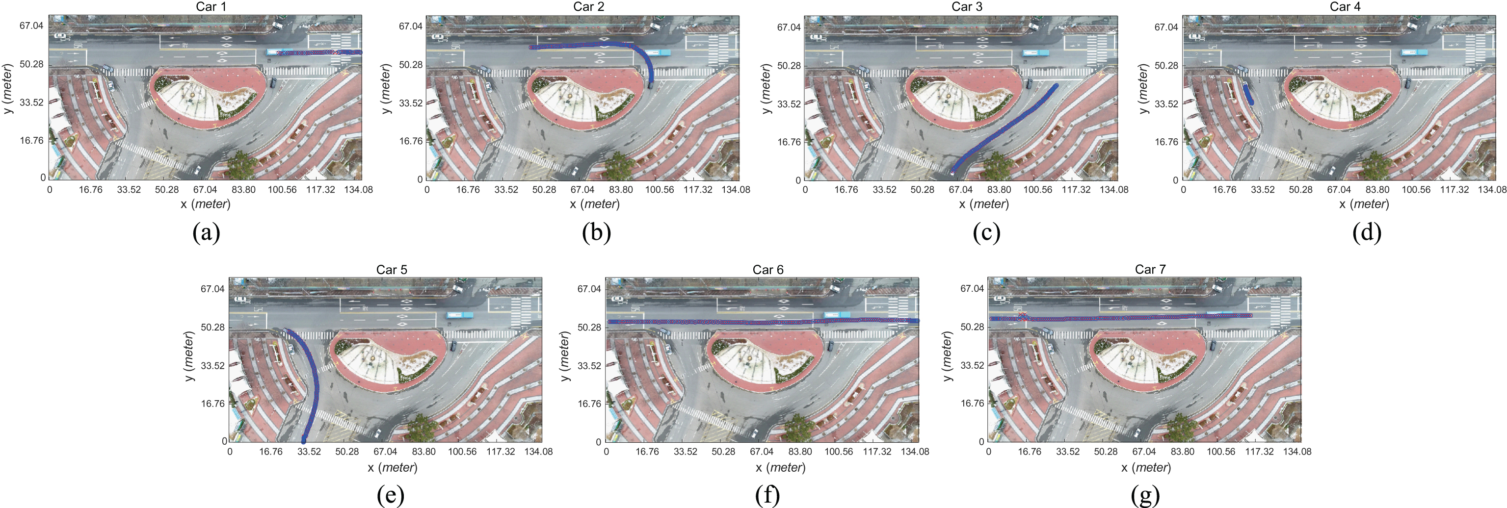
Figure 5 shows all the measurements of seven cars for 580 frames, including false alarms. The sampling time Δ in Equation (6) is 0.021 sec since the frame rate is 48 fps. The standard deviations of the process and the measurement noise are set at σ_x1 = σ_y1 = 30 m/s², σ_x2 = σ_y2 = 60 m/s², and r_x = r_y = 1.5 m, respectively; γ in Equation (17) is set at 16. The track is initializedby a two-point initialization method with speed gating, which limit the maximum speed of target by 30 m/sec [11]. Figure 6(a)-(g) are the results of Cars 1–7 tracking, respectively.

Fig.5

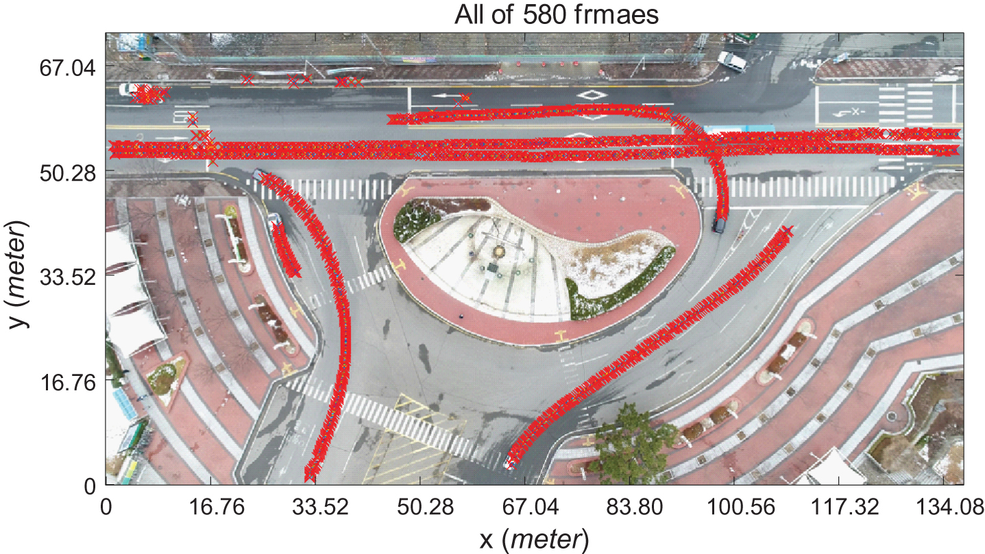
Measurements including false alarms for 580 frames.

Fig.6

Tracking result when Δ= 0.021 sec, (a) Car 1, (b) Car 2, (c) Car 3, (d) Car 4, (e) Car5, (f) Car 6, (g) Car 7.

The sampling time is set differently in the following experiments. Figure 7 shows the tracking result with Δ= 0.063 sec, that is, measurements are acquired every third frame from the original data. Cars 1–7 are initialized by the first and the forth frames. Figure 8 is the tracking results with every sixth frame (Δ= 0.125 sec) updated. Figure 8 is the tracking results with every eighth frame (Δ= 0.167 sec) updated.

Fig.7

Tracking result when Δ= 0.063 sec, (a) Car 1, (b) Car 2, (c) Car 3, (d) Car 4, (e) Car5, (f) Car 6, (g) Car 7.

Fig.8

Tracking result when Δ= 0.125 sec, (a) Car 1, (b) Car 2, (c) Car 3, (d) Car 4, (e) Car 5, (f) Car 6, (g) Car 7.

Figure 10 shows the ground truth of positions of Cars 1–7. Table 2 shows the root mean-squared error (RMSE) of the position. The large RMSEs of Cars 1, 6, and 7 are mostly caused by false alarms. RMSE is similar for 1, 3, and 6 sampling steps, but becomes larger when the sampling step is 8.

Fig.9

Tracking result when Δ= 0.167 sec, (a) Car 1, (b) Car 2, (c) Car 3, (d) Car 4, (e) Car5, (f) Car 6, (g) Car 7.

Fig.10

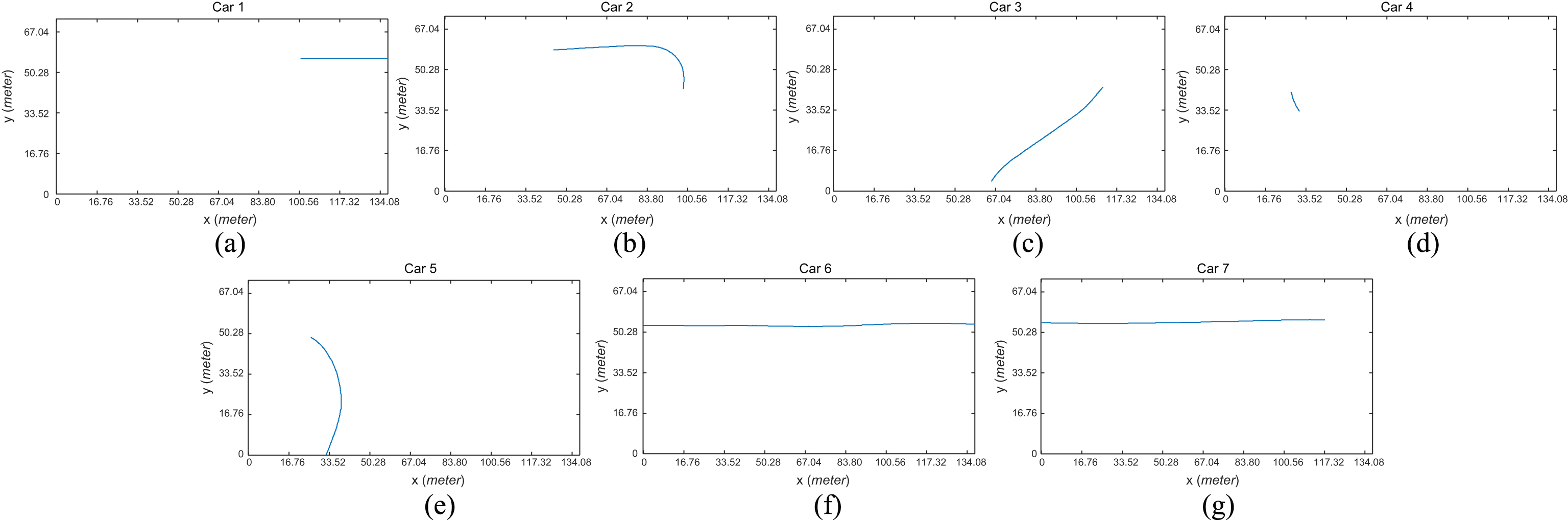
Ground truth, (a) Car 1, (b) Car 2, (c) Car 3, (d) Car 4, (e) Car 5, (f) Car 6, (g) Car 7.

Table 2

Root mean-squared error (RMSE) (meter)

Δ	Car 1	Car 2	Car 3	Car 4	Car 5	Car 6	Car 7	Avg.
0.021	2.02	0.66	0.7	0.16	0.8	1.65	1.67	1.1
0.063	2.17	2.03	0.7	0.19	1.47	2.53	1.66	1.54
0.125	2.23	0.64	0.7	0.2	2.14	3.4	1.69	1.57
0.167	9.68	0.67	2.34	1.85	3.37	4.03	1.65	3.37
Avg.	4.02	1	1.11	0.6	1.95	2.9	1.67	1.89

5 Conclusion

In this paper, multiple moving objects are captured from a long distance by a drone. The locations of objects are detected using frame difference. Seven targets are tracked with IMM filtering. Experimental results show that the proposed algorithm detects and tracks moving objects with good accuracy. More complicated scenarios where targets are closely located may require more advanced data association techniques, which remain for future study.

Footnotes

Acknowledgments

This research was supported by Basic Science Research Program through the National Research Foundation of Korea (NRF) funded by the Ministry of Education (Grant Number: 2017R1D1A3B03031668).

References

Hampapur

, Brown

, Connell

, Pankanti

, Senior

A.W.

and Tian

Y.-L.

, Smart Surveillance: Applications, Technologies and Implications, IEEE Pacific-Rim Conference On Multimedia, Singapore, 2003.

Kumar

et al., Aerial video surveillance and exploitation, IEEE Proceedings of the IEEE89(10) (2001).

Chung

, Kim

Y.-J.

and Kim

, A two-stage foreground propagation for moving object detection in a non-stationary, IEEE AVSS (2016), 187–193.

Yeh

C.-H.

, Lin

C.-Y.

, Lai

H.-E.

, Muchtar

and Sun

M.-T.

, Three-pronged compensation and hysteresis thresholding for moving object detection in real-time video surveillance, IEEE Trans on Industrial Electronics64(6) (2017), 4945–4955.

, He

and N

, Moving object detection with a freely moving camera via background motion subtraction, IEEE Trans on Circuits and Systems for Video Technology27 (2017), 236–248.

Mousse

, Motamed

and Ezin

, An Adaptive Algorithm for Fast Moving Object Detection from Dynamic Background based on Codebook, International Conference on Robotics and Mechatronics, 2016, pp. 584–588.

Zhang

, Huang

, Li

, Liu

, Zhang

and Xing

, Research of Moving Object Detection Algorithm in Transmission Lines under Complex Background, International Conference on Condition Monitoring and Diagnosis, vol. 30, 2016 pp. 176–179.

Olugboja

and Wang

, Detection of Moving Objects using Foreground Detector and improved morphological filter: 2016 3rd International Conference on Information Science and Control Engineering, Vienna International Hotels, Beijing, China, 2016.

Yeom

, Lee

M.-H.

and Cho

I.-J.

, Long-range Moving Object Detection based on Background Subtraction ISIS2017, 2017, pp. 1082–1085.

10.

Lee

M.-H.

and Yeom

, Vehicle Tracking based on Kalman filtering with drone imaging, ICGHIT2018, Session IV-1.5, 2018.

11.

Lee

M.-H.

and Yeom

, Detection and Tracking of Multiple Moving Vehicles with a Drone, to be submitted, 2018.

12.

Bar-Shalom

, Li

X.R.

, Multitarget-multisensor Tracking: Principles and TechniquesCT, YBS Publishing1995.

13.

Stone

L.D.

, Streit

R.L.

, Corwin

T.L.

, Bell

K.L.

, Bayesian Multiple Target Tracking 2nd, Artech house, Boston, 2014.

14.

Bar-Shalom

, Li

X.R.

, Kiruba

Estimation with Applications to Tracking and Navigation.

15.

Yeom

, Kiruba

and Bar-Shalom

, Track segment association, fine-step IMM, and initialization with doppler for improved track performance, IEEE Transactions on Aerospace and Electronic Systems40(1) (2004), 293–309.

16.

Gonzalez

R.C.

, Woods

R.E.

, Digital Image Processing 3rd, Pearson Prentice Hall, New Jersey, 2008.