Accounting for composite travel time distributions within a traffic stream in determining Level-of-Service

1. Introduction

Bimodal and Multimodal distributions of travel time have been observed in a number of settings. These include arterials [1, 2], due to the presence of signalized intersections, and freeways [3–5] when there are lane closures during construction periods or, more generally, when both congested and uncongested travel is present. These multimodal distributions reflect different subgroups of traffic which may experience different service quality along the same roadway. Previous studies have used Expectation Maximization and hierarchical Bayesian mixture models to separate these distributions in order to develop travel time reliability indices [1–4].

In this paper an Expectation Maximization algorithm [6] is utilized to separate multimodal travel time data collected on a major arterial (Jimmy Carter Boulevard) in the metropolitan Atlanta, Georgia area and assign a separate corridor-level LOS rating to each distribution. This multiple LOS rating method is not intended to replace the HCM 2010 facility LOS method [7], instead it is being developed as a supplementary tool to provide more detailed LOS information. For example, the impact of roadway improvements (e.g., signal timing, geometric changes, etc.) on the different road user subgroups may be directly evaluated by providing a more detailed view that captures the underlying performance of each subgroup rather than a single aggregate LOS measure. This type of analysis is enabled by the growing availability of continuous data collection systems such as Bluetooth ^®, cell phone tracking, etc. The advantages and drawbacks of this approach are discussed later in the text.

2. Previous research

As mentioned earlier, bimodal/multimodal travel time distributions have been encountered on multiple roadway types [1–5]. Typically, these distributions have been studied in association with research on travel time reliability and/or congestion detection. For example, two previous studies aimed to develop congestion detection algorithms for arterial roadways [1, 2]. Ji and Zhang successfully used bus probe data to collect travel times along an arterial roadway on the Ohio State University campus by recording from the campus bus Automatic Vehicle Location (AVL) system. In this study, location data near bus stops were omitted in order to collect travel time data on segments which included either one signal or no traffic signals and did not include delay from boarding and alighting. It was found that the segments with one signal consistently showed bimodality in travel times while a segment without a signal had only a single mode. The resulting data were curve fit using a Bayesian mixture model assuming either a single or bimodal distribution then congestion detection algorithms were applied. In the segments with a signalized intersection, the congestion detection algorithms developed detected congestion more accurately with the bimodal models than the single mode models [1].

In a second study by Yang et al. similar data were collected on multiple corridors in the downtown area of Nanjing, Jiangsu province in China. The selected links were similar to Ji and Zhang’s study in that each link only contained one signal. Similarly, bimodal distributions were found and an Expectation Maximization (EM) algorithm was used to separate the data. In this study a combination of six distribution types were tested on each data set and the best fit for each distribution found based on the resulting R-squared values. Subsequently, the resulting distributions were applied to two methods of detecting congestion in bimodal travel time distributions; the Expected Travel Time and RATIO indices [2]. Additionally, Henclewood et al. suggested that although first moment values, such as average travel time may be sufficient to evaluate general traffic performance at an aggregated level, considering travel times at the distribution levels allows for a better representation of traffic performance at an individual vehicle level [8].

Freeway studies have also found bimodal travel time distributions [3, 4]. Park et al. created a model to predict congested and uncongested freeway travel times similar to weather forecasting. In this study, simulated data were used from a model of I-66 outside of Washington, DC. Using this model, congested and uncongested conditions were simulated separately and data from the different simulation runs intentionally mixed. Here, varying ratios of congested travel time data and uncongested travel time data were mixed and separated using Expectation Maximization algorithms. Travel time data for all vehicles completing the route were available so the ratio of congested to uncongested data was known before bimodal curve fitting. After separating the data, the output ratios from the Expectation Maximization algorithm were found to be very similar to the known input conditions. Their conclusion was that if a high enough sampling rate could be attained on freeways, the ratio of congested to uncongested travel times during periods of the day could be accurately estimated. Therefore, these ratios, developed using historical data, could be used to give drivers the probability of encountering congestion during a given time, on a given route, and provide an estimate of congested and uncongested travel times [3]. These multimodal distributions have also been found, by Colberg et al., to occur on freeways in work zones when lane closures are present. In this study it was found that drivers in the left lanes of the study corridor (the location of the lane closures) experienced significantly shorter travel times than those in the right lanes of the same freeway. It was believed that vehicles in the right lanes experienced higher delays due to queue formation in the right lanes and that slower-moving trucks were not permitted to travel in the left lanes [5].

3. Travel time data collection

The travel time data used for this study were collected along Jimmy Carter Boulevard, a major arterial, at and near its intersection with I-85 in the northeastern portion of the Metro-Atlanta, GA area. Data collection was initiated using pole-mounted Bluetooth ^® detection units at the six locations illustrated in Fig. 1. These Bluetooth ^® units are being used to collect travel time data on 20 routes through the corridor focusing on paths ending or beginning at the I-85 freeway interchange. For this analysis, the paths of interest are from the north end to the south end of the Jimmy Carter Boulevard corridor, a distance of 2.4 miles (4 km) and the reverse path.

OPEN IN VIEWER

Fig. 1.

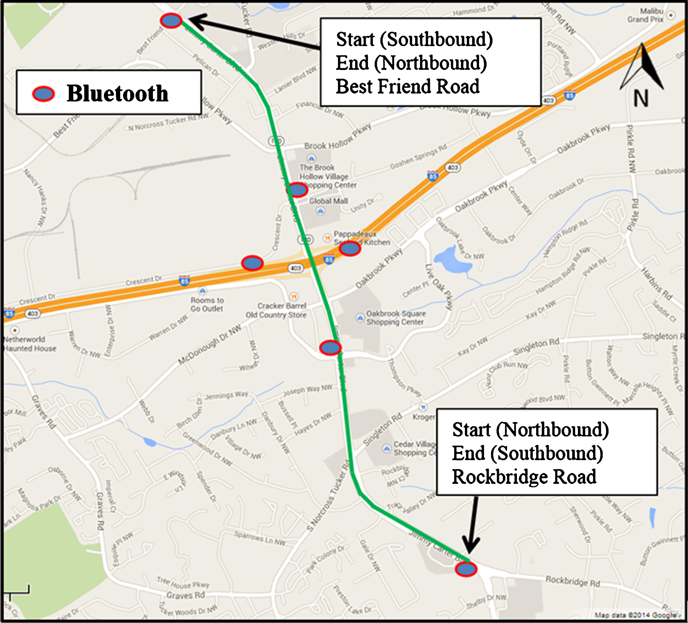
Jimmy Carter Boulevard Bluetooth ^® detector unit locations.

Due to the low detection rate of Bluetooth detectors [9, 10], it is difficult to perform analyses and identify patterns over short (e.g. one hour) intervals and successful analysis often requires combining data from multiple days. For this study, data were segregated into five data sets; one for each day of the week. The individual datasets comprised 14 days of data, collected over a 16-week period excludes data collected during the week of a major U.S. holiday (Labor Day).

Arterial roadway travel times often exhibit bimodal or multimodal travel time distributions. This is typically caused by the signal systems in place along these corridors [1, 2]. It is well known that coordinated signal systems may systematically enforce groupings of vehicles into different travel time bands. For example, one group of vehicles may be able to traverse the entire corridor stopping only once due to a red signal while another vehicle group may traverse the same corridor and encounter multiple red signals. In this instance, the vehicles that stop multiple times will have more delay and a longer travel time than vehicles that stop only once. Another source of these multiple distributions may be congestion and delays due to lane specific conditions. For example, spillback from left turn lanes into through lanes may cause added delay to through vehicles traveling in the lanes adjacent to the left turn lanes. For instance, in the corridor studied for this effort left turn lane spillbacks have been witnessed by the research group along the study corridor during congested periods. Additional potential causes for multimodal travel time distributions exist, such high driveway densities, lane additions and drops, etc.

Figure 2 illustrates the observed travel times over the study period for the southbound (Tuesday, 8AM to 9AM) and northbound (Tuesday, 7AM to 8AM) through movements respectively. In this figure, data-points represent a single paired (origin-destination) observed travel time with the varying colors representing different measurement days. These data sets have been pre-processed with two filters. The first filter is a “20 minute filter” that removes any travel time observation greater than 20 minutes. The second filter is a “60 miles per hour” filter that acts to remove any observed travel time that when converted to a speed is greater than 60 miles per hour. These filters removed data likely resulting from well-known issues associated with travel time data collected using Bluetooth technology ^® [5, 12] and are considered well outside the reasonable travel time range for this corridor. In all cases the number of removed data points was minimal.

OPEN IN VIEWER

Fig. 2.

Travel times for through movements along the study corridor (a) Southbound Travel Times (AM peak), (b) Northbound Travel Times (AM Peak).

Observing Fig. 2(a) and 2(b) it is difficult to visually discern any obvious “banding” of travel times. However, in the histograms for these data shown in Fig. 3, for the south-bound direction there are three (possibly four) discernable travel time bands: the first centered at slightly less than 6 minutes, the second at slightly less than 8 minutes, and the third (and fourth) at greater than 8 minutes. For the northbound direction, three travel time bands are apparent, the first is centered at just less than 4 minutes, the next at near 5 to 6 minutes, and a third from approximately 7 minutes onward with some outlying observations at longer times.

OPEN IN VIEWER

Fig. 3.

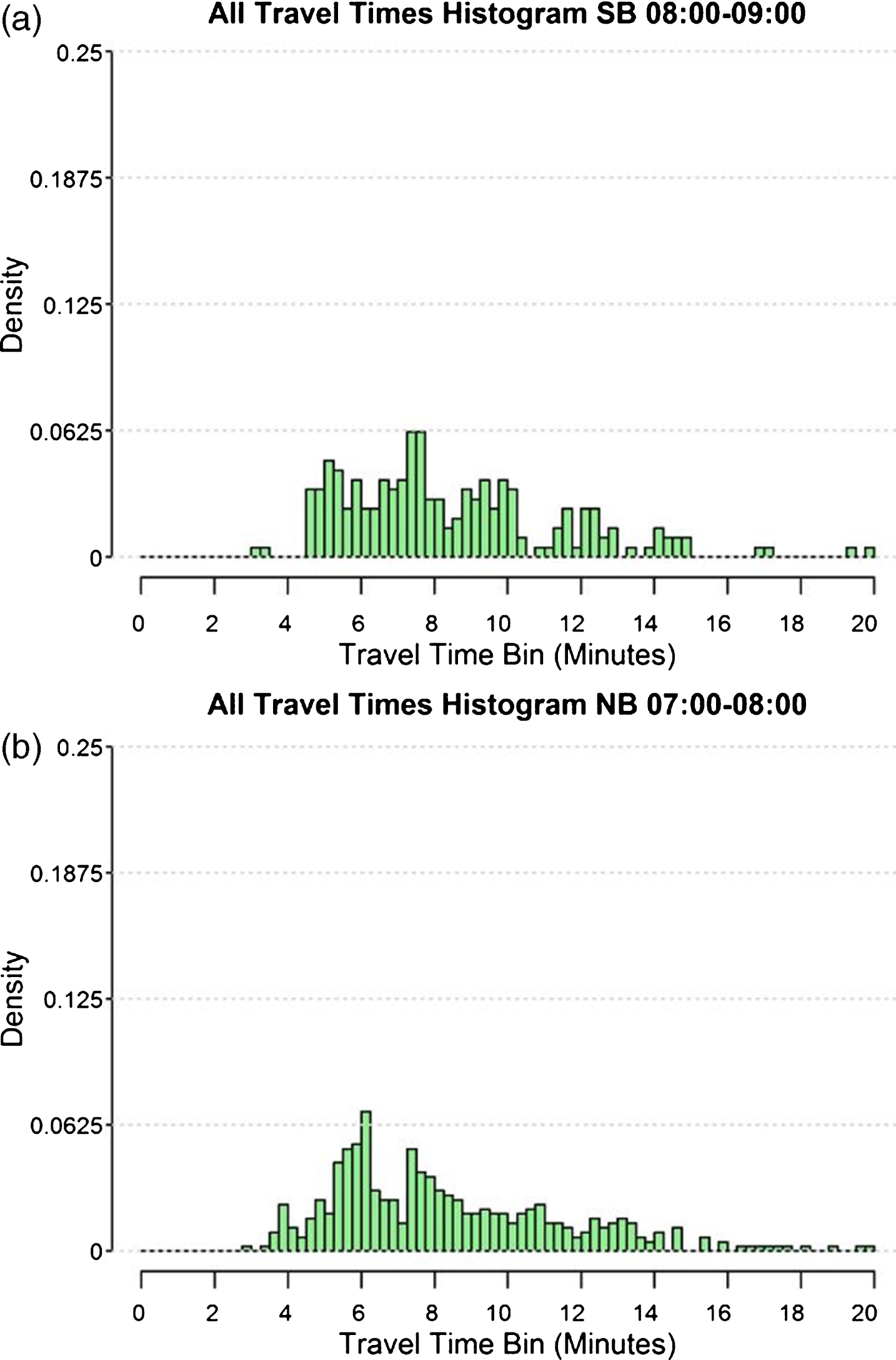
Travel time histogram of data (a) Southbound histogram, (b) Northbound histogram.

The multiple peaks (modes) displayed in the histograms are strong evidence for the existence of multiple travel time distributions. To identify the characteristics of these individual distributions, multiple gamma curves were fit to the observations. In order to accomplish this, an Expectation Maximization algorithm for multiple gamma curve fitting was used. This algorithm, named the gammamixEM function, is part of the “mixtools” package that was developed and implemented in R by Bengalia et al. [6]. This function uses the Expectation Maximization iterative process to fit multiple gamma curves and provides a posteriori probability for each data point (i.e. the estimated probability that the point belongs to a particular distribution).

These probabilities were used, in conjunction with a random number generated between 0 and 1, to assign individual data points to a particular distribution. It should be noted that since three distributions were fit, three posterior probabilities were generated for each data point, the sum of which equals one. Finally, Fig. 4 shows the fitted gamma curves for each travel time band and the histograms of the data assigned to each distribution for the southbound direction. In general, it was seen that multi-distributional fit provided a meaningful improvement in the coefficient of determination relative to a single mode distribution. For example, for the data shown in Fig. 3 the coefficient of determination increased from about 0.95 to 0.99 for the northbound data and from 0.98 to 0.99+ for the southbound data. Both of these improvements are significantly greater than that expected randomly by the increase in fitting parameters.

OPEN IN VIEWER

Fig. 4.

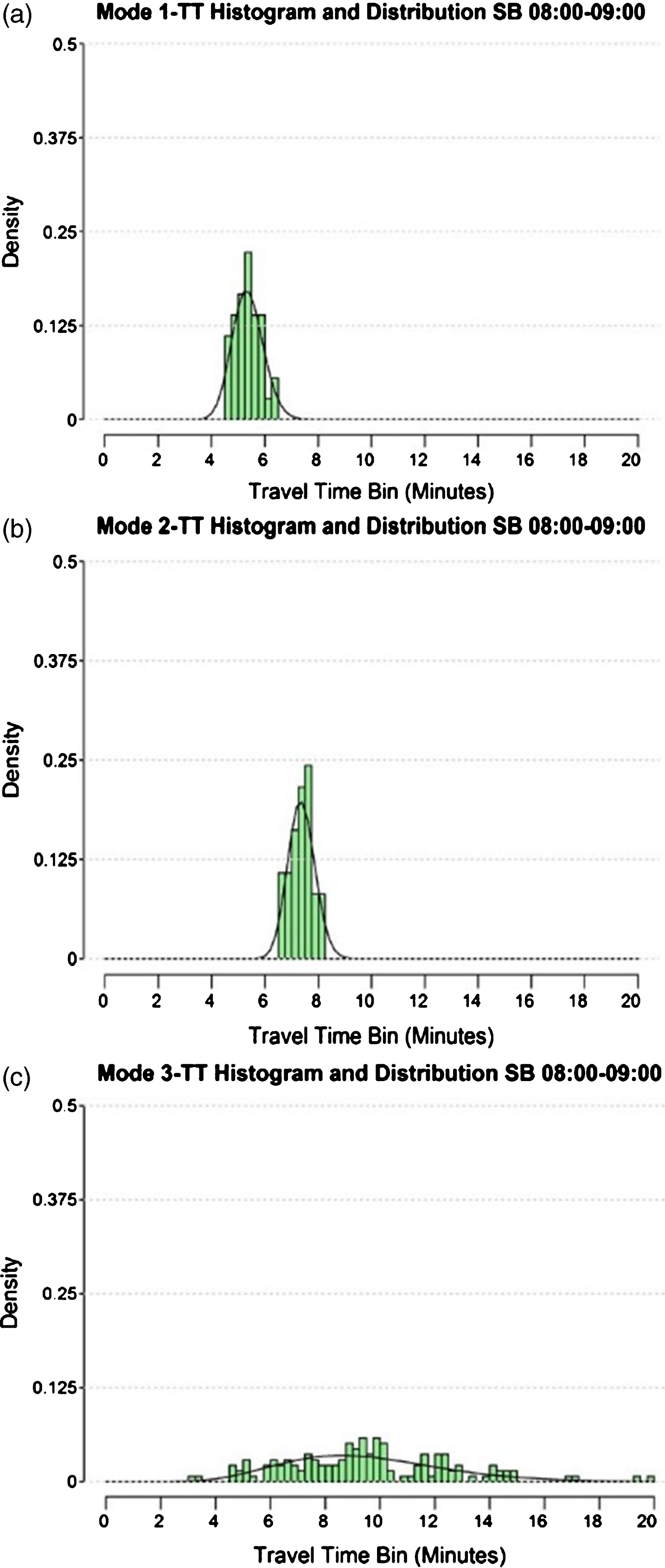
Travel time data separated for southbound (a) Distribution 1, (b) Distribution 2, and (c) Distribution 3.

After assigning multiple gamma functions to the data sets and separating the data by distribution, an LOS rating was assigned to each distribution. In order to assign an LOS rating for each distribution a base free flow speed for each direction was first determined. The HCM methodology for determining the facility LOS rating was followed when determining the base free flow speed [7, 13]. A base free flow speed was not field measured as the given Bluetooth ^® data includes control delays and does not allow for distinguishing free flow speeds on a corridor [14].

Travel speed through the corridor was derived from the travel time data distributions. For each distribution created through the curve fitting procedure, the average travel time was converted into a speed in miles per hour. The final step in determining facility LOS was to calculate the percent reduction of free flow speed for each individual mode and determine which speed reduction range included the observed reduction.

Table 1 shows the percentile ranges for each LOS rating according to the 2010 HCM [7]. The multiple facility LOS ratings for the lowest speed hour for AM and PM periods can be found in the results section in Tables 2 and 3. In the HCM method of analysis a v/c ratio greater than 1.0 automatically warrants an LOS of F as can be seen in Table 1. In this study, volume counts were not available thus, for this analysis, v/c ratio was not considered when deter-mining LOS ratings.

For brevity, shown here are the hour with the lowest average morning speed and evening speed, by direction, for each day of the week, essentially using lowest mean speed as a surrogate to identify the peak hour as volume data are not available. However, given the continuous nature of the Bluetooth ^® data, a similar analysis can be completed for each hour of the day or any chosen time range. Table 2 shows the LOS and mean speed for each modal distribution and overall, corresponding hour of the day, day of the week, and direction along the corridor for the AM period. Table 3 shows the results for the PM period. LOS ratings are generally lower for the PM than the AM. Interestingly, the lowest PM speeds were consistently observed from 5PM to 6PM for the Southbound direction, except for Friday which occurred from 4PM to 5PM.

During the AM period (Table 2), the lowest mean speeds were typically observed between 8AM and 9AM for the southbound direction and 7AM to 8AM for the northbound direction, except for Thursdays in the southbound direction when the lowest average speeds occurred between 7AM and 8AM. During the AM period, the vehicles in Mode 1 (the fastest group) typically experienced a LOS of C or D for southbound travel and a LOS of B or C for northbound travel. Mode 2 vehicles (the intermediate speed group) experienced LOS C, D, or E, and the slowest group (Mode 3) experienced a LOS of E or F. The overall LOS rating for both directions during the AM peak is a D except for Wednesday in the northbound direction which is E. In 4 cases this is worse than that observed for Mode 2 vehicles, in 3 cases the same, and in 3 cases better.

During the PM periods (Table 3), the lowest mean speeds were typically observed, between 5PM and 6PM for the southbound route except on Friday when the southbound minimum speed occurred between 4PM and 5PM. Northbound speeds reached a minimum between 3PM and 4PM. In this period, the fastest speed group typically experienced an LOS of D or E for southbound travel and C or E for northbound travel. The middle group experienced LOS D, E, or F, and the slowest group experienced mostly an LOS of F, except northbound on Thursday which experienced an LOS of E. The typical overall LOS rating for both directions during the PM peak is an E except on Friday for both directions when it is an F. In 4 cases this is better than the middle (Mode 2) distribution, in 4 cases the same, and in 2 cases worse.

Mode 3 vehicles, the slowest group, experienced minimum average speeds ranging from 10.4 mph to 16.1 mph (travel times of 13.8 minutes to 8.9 minutes) during for the AM peak period. During the PM periods drivers in Mode 3 experienced minimum average speeds ranging from 7.5 mph to 13.5 mph (travel times of 19.1 minutes to 10.6 minutes). From Figs. 5 and 6 it can be seen that there are a significant portion of vehicles in this slowest distribution. During peak periods it is plausible that many of these are actual travel times from vehicles that do not stop along the corridor but experience severe congestion pushing them into the slowest distribution. However, during non-congested periods of the day this distribution carries fewer data points but does not disappear. There are 98 driveways and 12 signalized intersections from which a driver may access many businesses ranging from office complexes to restaurants. Due to the high number of destinations along the corridor it is possible that members of the Mode 3 distribution may also have stopped for a few minutes along the corridor.

OPEN IN VIEWER

Fig. 5.

Overall and modally separated data: Southbound direction.

OPEN IN VIEWER

Fig. 6.

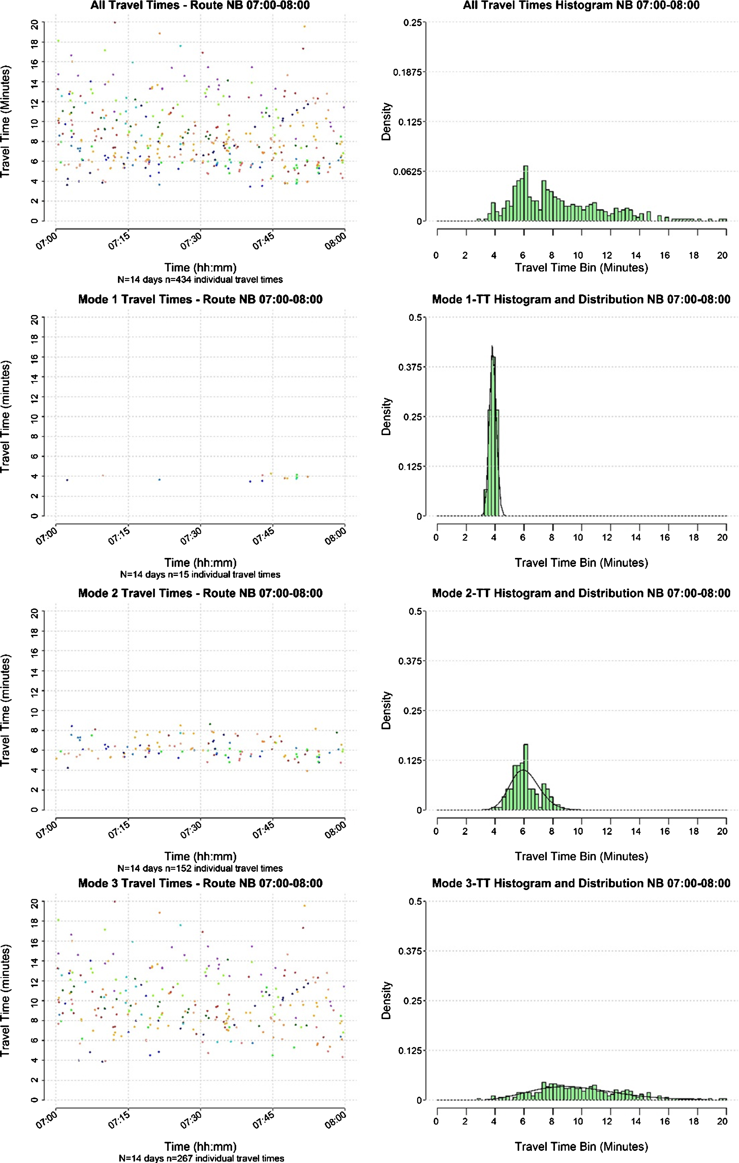
Overall and modally separated data: Northbound direction.

Despite this potential mix of vehicles in mode 3, these data remain informative. When short stops (e.g. to refuel) are the primary reason for the long travel times, which is likely during uncongested traffic, one would expect similar behavior in a before-after analysis, allowing for separation of this group in any improvement analysis. Thus, for example, where only signal timing has changed these vehicles should not be considered when using Bluetooth ^® data to compare before-after results as their behavior is likely not a function of the signal timing. During congested conditions this mode may contain a mix of vehicles that experience high delays and vehicles with short stops. Where improvements are not anticipated to impact the number of vehicles making stops changes in this modes distribution will partially reflect the impact of improvements on highly delayed vehicles. In addition, fewer samples in the mode in an after data collection case will indicate fewer highly delayed vehicles.

It is believed that the fastest (Mode 1) and middle (Mode 2) groups of drivers likely drove the corridor continuously without stopping except where instructed to do so by traffic control devices. Approximately 34% to 38% of the data points lie within these two distributions. Although a uniform sampling rate over all road user sub groups cannot be assumed (discussed below), it can be assumed that a proportion of vehicles traversing the corridor fall into these two distributions. For the Southbound direction shown in Fig. 5, these distributions are separated by approximately 1.5 minutes or 90 seconds. For the Northbound direction shown in Fig. 6, these distributions are separated by approximately 2 minutes or 120 seconds. During the time period shown in Figs. 5 and 6 the signal-timing cycle length along the corridor is 140 seconds. These differences are likely related to different paths through the time space diagram as a function of signal offsets, vehicle arrival times, and congestion (potentially lane specific). For example, significant lane specific delays were observed in the field during the peak periods as left turning vehicles at some signalized intersections, especially near the I-85 interchange, spill back out of the left turn lanes into adjacent left-most through lanes. However, the intent of this analysis is not to determine the reason for the different behaviors but instead highlight that different road user sub groups are experiencing different LOS. Improved analysis and evaluations (e.g. before-after comparisons) may be obtained by considering these groups separately rather than as a single aggregate collection of road users.

The concept of multiple LOS rating assignment can be used to give a more detailed description of traffic conditions. There are two scenarios that affect how the multiple LOS ratings can ultimately be used for public reporting. Under the first assumption, there is a uniform travel time sampling rate over all road user sub groups of the corridor of interest, and under the second assumption, a uniform sampling rate cannot be reasonably assumed (e.g. the first assumption cannot be proven). These two situations and their future exploration will be discussed in the next two sections.

Scenario One: Uniform Sampling Rate Over All Road User Sub Groups

This approach implicitly assumes that the sample data were collected uniformly across all road user sub groups (that is, each of the underlying gamma curves is sampled at the same rate). In the case where a uniform sampling rate across all sub groups can be assumed, proportions of vehicles in each distribution can be accurately estimated and presented along with the LOS for that distribution. Thus, the multiple LOS rating information will become more robust in describing traffic patterns and situations. Furthermore, if using the multiple LOS method as a performance measurement tool for before and after project implementations, one can see clearly not only the shifts and changes in distributions on a statistical level but a shift in the percentage of drivers be-longing to each distribution.

Scenario Two: Cannot Assume Uniform Sampling Rate Over All Road User Sub Groups

When it cannot be reasonably assumed that there is a uniform sampling rate over all road user sub groups the multiple LOS method is not as robust as the percentages of drivers in each distribution cannot be assumed to be the same as the sampling proportions. In this situation it can only be assumed that the different distributions exist within the data set and that there are certain un-known proportions of vehicles experiencing different levels of service depending on combinations of red or green signals encountered while traversing the corridor. In the case of the data set used for this research project, a uniform sampling rate across road user subgroups cannot be safely assumed as the likelihood of a Bluetooth ^® data point is related to vehicle speed and distance from the detector as well as other factors. When using multiple LOS ratings as performance measures for before and after analyses, one can use the separated data sets as individual distributions and run robust statistical tests to determine if changes in the distributions are statistically significant (e.g. using t-tests, chi-squared tests, etc.). Typically, statistical tests apply only to a certain distribution type assumed by the analyst. When these tests are applied to data that clearly has multiple distributions the test results cannot be taken as accurate as would be the case with the aggregated travel time distributions. Using these data separation techniques one can test the significance of shifts in the separated distributions. This can also be useful as a change may not affect the LOS ratings, however, the statistical tests may show statistically significant changes in the distribution proving that an improvement did occur due to changes made in the corridor.

9. Conclusions

Separation of the mixed distributions allows for robust statistical testing of the separated data. However, under the conditions that a uniform sampling rate can be assumed, proportions of vehicles in each distribution can be accurately estimated and shown along with the corresponding LOS ratings to give a more comprehensive picture of traffic conditions to non-transportation professionals. In the case of Jimmy Carter Boulevard in northeast Atlanta, Georgia, it was found that the highest speed distribution in morning’s slowest speed periods exhibited a range of LOS B, C, and one D rating while the afternoon highest speed distribution exhibited LOS C, D, or E ratings. The second distribution in the morning showed a variety of C, D and E LOS ratings depending on the day, while in the afternoon D, E and F LOS ratings were experienced. During the peak periods a significant portion of travel times fall into the third (slowest) distribution. It is plausible that the third distribution during the peak periods is composed of a portion of travel times where drivers did not make any stops in the corridor but were pushed into this distribution by severe congestion. The third distribution, however, is mixed with outlying data points where drivers may have stopped as there are ample opportunities (98 total driveways) for drivers to stop along the corridor. During off peak periods the third distribution contains a much smaller proportion of the travel times, suggesting that these are mostly composed of travel times where drivers stopped at a destination along the corridor for a short period of time.

Multiple curves were fit to the travel time data sets in this paper using an Expectation Maximization (EM) algorithm for gamma curves. The data were separated using the posterior probabilities calculated by the R statistical package “mixtools” using the function “gammamixEM” function. LOS ratings were assigned using a method based off of the HCM 2010 manual. In this method, the base free flow speed was calculated according to the HCM 2010 manual, and average travel times for each distribution were calculated and converted to a speed in order to use as the travel speed in determining the multiple LOS ratings. The HCM recommended percentile thresholds for facility LOS ratings were used to assign each distribution an LOS.

Previous studies have found usefulness in separating multiple distributions for research in travel time reliability indices. This paper found usefulness in separating the travel time data to assign multiple LOS ratings to the different distributions. From the analysis it was clear that different subgroups of vehicles can experience different LOS rating on the same roadway facility during the same time period. By separating the travel times into its underlying distributions it becomes possible to consider each of these subgroup separately. It was also found that separating these distributions allows for more robust statistical tests to be used to detect changes in before and after studies. This type of analysis will be used in the future to test the effects of a new interchange being constructed on the Jimmy Carter Boulevard corridor.