Nonlinear tool traces fast tracing algorithm based on single point laser detection

Abstract

There are lots of line traces on the surface of the broken ends which left in the cable cutting case crime scene along the high-speed railway in China. The line traces usually present nonlinear morphological features and has strong randomness. It is not very effective when using existing image-processing and three-dimensional scanning methods to do the trace comparison, therefore, a fast algorithm based on wavelet domain feature aiming at the nonlinear line traces is put forward to make fast trace analysis and infer the criminal tools. The proposed algorithm first applies wavelet decomposition to the 1-D signals which picked up by single point laser displacement sensor to partially reduce noises. After that, the dynamic time warping is employed to do trace feature similarity matching. Finally, using linear regression machine learning algorithm based on gradient descent method to do constant iteration. The experiment results of cutting line traces sample data comparison demonstrate the accuracy and reliability of the proposed algorithm.

Keywords

Signal detection wavelet transforms lasers machine learning

1. Introduction

High-speed railways are being developed rapidly in China. To ensure long-term stability of infrastructure, lots of cables, such as leaky cables, signal cables, rail vehicle cables, and grounding wires, are distributed along the railway. The inner conductors of many cables are made of copper, a coveted target of criminals due to its high economic value. In recent years, frequent theft of cables along the high-speed railways has resulted in huge losses of state property and has caused interruption of railway signals and communication equipment power supply. This has forced failure of the respective systems leading to several railway accidents, significant loss of lives, and diminished safety of property [1].

Statistical data show that criminals use wire cutters, cable cutters, destroy pliers, and other large shear tools to sever cables. Line traces, which are scratches on the surface of the body, can be caused by the pressure of the line-shaped deformation and line traces of the broken ends on the surface are frequently found at the scene. Thieves use tools that cause load on the trace-bearing body, which form local material changes on the contact part. Moreover, thieves use tools to cut the cables, which form local material changes on the contact part. The tool traces reflect the external morphological structure of the contact area, and provide clues to the investigation based on the analysis of the tools used in the criminal act, thus narrowing the scope of the investigation. It possesses characteristics that are difficult to destroy or disguise, frequently occurring, and possess high identification value for investigators to determine the nature of the case and the tools used in the criminal act. These characteristics are important to confirm suspects [2].

Compared with the traditional methods of observation and comparison, the nonlinear shear trace quantitative examination in image recognition and 3D scanning technology, Kassamakov which emerged in recent years, provides a new solution. Gambino et al. [3] from The City College of New York in the USA used a white light confocal microscope to measure linear trace surface ripple data. They subsequently used principal component analysis to collect data for dimension reduction. They also used support vector machines and conformal prediction algorithms for similarity comparison. The effectiveness of this method is proven by using multiple sets of scratched line trace samples. Baker et al. [4] from the Netherlands Forensic Institute in Holland constructed a multi-scale registration frame for needle-line traces. The effectiveness of this method is verified by the actual line trace comparison experiment. Kassamakov et al. [5] from Fraunhof’s information and data processing research in Germany investigated tool scratch traces, extracted traces from the groove, positioned the groove based on the template-based approach, and calculated the degree of connection between two grooves through related analysis. Yang et al. [6] from Guangdong Police College conducted tool trace texture signal analysis using discrete wavelet transform and constructed a local wavelet energy feature vector. The trace similarity test was performed by measuring the standard deviation of the features. Wang [7] from Shenzhen University used fractal dimensions to quantify the characteristics of the surface shape of line traces and established fractal dimension group identification rules, which are distinguished automatically. The effectiveness of this method is verified by the bolt cutter shearing edge trace experiments. However, these detection methods are complicated because of the randomness at the crime scene. The structure of the algorithm is not well suited to engineering. The pictures and size of 3D files are too large, increasing the difficulty and making the above method unsuitable as the first approach to handling the case, which greatly reduces its practical value.

The single-point laser displacement test has advantages that include an undamaged surface of the measured object, a light-free environment, high precision, small data file size, and good frequency response characteristics. Pan et al. [8] from Kunming University of Science and Technology reported a line trace detection laser signal adaptive matching algorithm in June 2015. This method can identify the “coarse and coherence” trend feature in trace detection signal data. It is a fitting method that involves quantitative characteristic vectors by cosine vector curve and can individually calculate sample spaces. Finally, the method uses a dynamic programming algorithm to compare the similarity in batches and match the maximum similarity of each sample [8]. However, the following problems are encountered when this method is applied to analyze the traces of actual sheared scene:

Signal noises reduction: The displacement picked up by the signal laser sensors is often mixed with many background noises restricted to the actual test environment and the difference between the broken ends of the cable itself. This type of noise arises from the mechanical error of the test equipment itself and external disturbances. To this end, the method requires maximum noise interference reduction and improvement of the quality and accuracy of the follow-up work based on the accuracy of the signal.

Signal Matching: There is a wide range in the shapes of the actual sheared traces. Despite the use of the same cutting tool, the broken ends will differ with respect to the number of directions and displacement deviations upon being severed. The lengths of the match signals and the signals to be matched are not the same. At the same time, the two trace detection signals are likely to coincide at only one part. In reality, the detection signal cut by the same tool cannot directly acquire its similar characteristics in the time domain; therefore, the data need to be converted to the transform domain for processing.

Tool inference: Due to rampant criminal activity, the scene of the incident may have hundreds of shear broken ends. The shear surface morphology of the cutting tool cannot be fully reflected in the broken ends of cables, except the part of the shear surface (an incomplete mark) that remains on the individual trace-bearing body. When comparing every data point, the computation involved in the algorithm will greatly increase, lowering the contrast efficiency. To do this, a fast comparison of the characteristics of a large number of trace laser detection data points by a dynamic time warping algorithm is required to implement the traceability inference of the cutting tool traces further.

From Based on previous research and in view of the requirements of efficient and rapid judgment of cutting tools in the actual scene, a fast traceability algorithm for nonlinear line trace features in the wavelet domain is designed. This algorithm uses a laser displacement sensor to detect signal characteristics and reduce noise using wavelet decomposition. Furthermore, the dynamic time warping algorithm is used based on the wavelet features to perform a similarity matching of trace features. Finally, correct determination of the corresponding tools is quickly achieved. The practicality and effectiveness of the proposed algorithm are verified by experiments involving the use of actual trace inference shear tools.

2. Detection of signal noise reduction

2.1. Overview of wavelet noise reduction

First, the single-point laser detection instrument described in literature is used to collect the non-contact data [2]. Then, the large amount of background noise interference contained in the laser detection signal is denoised to obtain a relatively stable coherent peak trend. Using wavelet noise reduction, the basic step is to perform a wavelet transform of the signal. The characteristics of the signal after wavelet transform are assigned to the wavelet transform coefficients of each scale. The relevant threshold is selected according to the analysis and wavelet transform coefficient, to ensure maximum suppression of background noise [9].

The basic steps involved in wavelet denoising are [10]:

Set up: $f (t) = s (t) + n (t), t = 1, 2, \dots, N$ (1)

Among them:

f (t) represents the signal data including noise

s (t) represents the original signal data

n (t) represents the noise signal data

The entire process of the noise reduction algorithm aims to remove the highest noise signal n (t) possible and reduce a part of the original signal data s (t).

Decomposing the wavelet signal and selecting the original wavelet and decomposition level. Wavelets of different scales are superimposed with different weighting coefficients. Wavelet decomposition coefficients containing noise are calculated.

Selecting the threshold r for coefficients of each layer by statistical calculation. The high-frequency noise signal is processed according to the threshold r. The processing procedures are as follows:

$c_{i} = {\begin{matrix} 0, | c_{i} | < r \\ g (c_{i}), | c_{i} | \geq r \end{matrix}$ , and g (c_i) for the processing function.

All coefficients of the signal wavelet decomposition are smaller than the threshold are set to 0, and wavelet coefficients larger than the threshold can also be handled properly.

The inverse wavelet transform is able to transform the processed signal data into the time domain noise reduction data after completing the coefficient removal.

2.2. Noise reduction of shear trace detection signal based on wavelet decomposition

The type of wavelet must be selected prior to noise reduction. The original signal has to be decomposed into several layers in the actual noise reduction process. When more layers are decomposed, the details of data processing will also increase, leading to more details being erased to eliminate more noise. Therefore, a balanced decomposition layer must be determined [11, 12].

In the process of decomposition, the original signal is generally decomposed into two parts. Assuming that the original signal is decomposed to n layer, the composition of the original signal can be described as follows: $f = a_{n} + \sum_{i}^{n} d_{i}$ (2)

The hierarchical information can be represented by Fig. 1. Each node in the graph corresponds to the original formula:

Fig.1

Lock diagram of the image measuring system.

a_i is the approximation of the nth layer and is represented by (1, 0) in Fig. 1.

d_i is the i layer of detail data and is represented by (i, 1) Fig. 1.

f is the original data and is represented by (0, 0) in Fig. 1.

Fig.2

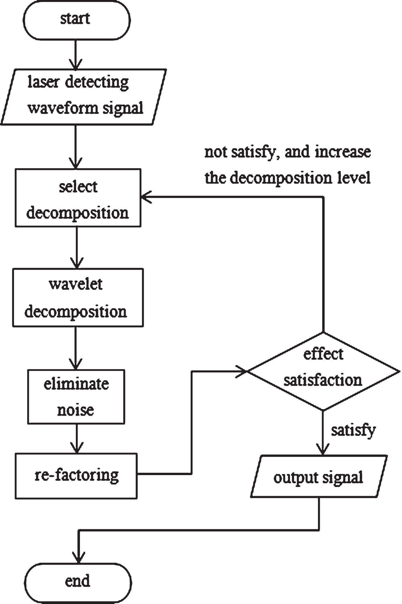
Flowchart of signal denoising.

Fig.3

Signal matching flowchart.

For the trace of the current detection, the approximate signal expansion of hierarchy 1 still has more glitches. The approximate signal expansion of hierarchy 2 has been greatly improved compared to the development of hierarchy 1. Most of the glitches have been improved, while the approximate signal of hierarchy 3 improves this phenomenon further and has been very close to the desired pattern from the graphical feedback. Therefore, only the development of hierarchy 3 is necessary in general.

According to the formula: $f = a_{n} + \sum_{i}^{n} d_{i}$ (3)

In addition to the approximate signal, detailed data are still needed. Although the approximate data are very close to the wave style according to the naked eye at hierarchy 3, signal details are still lacking because a significant amount of low amplitude noise is lost; therefore, it can only represent the general trend but cannot accurately show the traces. The signal should be filtered and denoised for every detail by setting a threshold:

$c_{i} = {\begin{matrix} 0, | c_{i} | < r \\ c_{i}, | c_{i} | \geq r \end{matrix}$ , c_i represents the ith decomposition of the wavelet coefficients.

IA threshold needs to be set and all data under the threshold must be removed to eliminate the noise in the detail. Given that general noise exists in high-frequency irregular pattern, the value is small, which is converted to the detail part. The signal should be filtered and denoised by setting a threshold for every detail. $f^{´} = a_{n} + \sum_{i}^{n} d_{i}^{´}$ (4)

Among them:

$d_{i}^{´}$ is the detail of the data after the threshold noise reduction.

$f_{i}^{´}$ is the trace data after the noise reduction.

Considering the characteristics of the shear line trace, the final selection is db4 or Haar as the mother wavelet through many experiments. Then, the decomposition and reconstruction of 2–5 layers are carried out according to the accuracy of the data detection. The waveform signal after the reconstruction of the removed noise is the denoised signal.

The flow chart of data noise reduction section is shown below:

The detection signal undergoes interference by the high-frequency noise because of the influence of mechanical vibration. Noise reduction is required to make the actual trace characteristic signal clear. The figure also shows that all high-frequency noise can be omitted after noise reduction, while the qualified data portion is uninterrupted.

3. Signal characteristic matching

3.1. Variable length and partial overlap problem

Prior to the matching the similarity of trace signals after noise reduction, the following two issues must be addressed [13]:

Variable trace length. Each collection of trace detection signal length is not the same. Most of the length of the matching signal data and the signal to be matched is different. At this time, the similarity of two discrete sequences can not be directly measured using Euclidean distance and correlation coefficients. Thus, point-to-point operations become meaningless.

Parts overlap. This means that two detection signal traces may only overlap at some part by coincidence. This condition can cause significant interference to the calculation of the final coincidence.

Therefore, the problem of variable length and overlap can be optimized through a computing algorithm capable of matching. The basic steps are as follows:

Setting the input data of A and B, which are data that satisfy the above requirements.

Setting a match to the minimum length L. The two coincidences must meet the minimum overlap length by selecting the longest length to the shortest part from A and to compare with B, that is equivalent to choosing a different location for a number of matches.

Iteratively executing each position’s contrast. Each comparison should be compared to the variance size of differences degree of the two corresponding positions. The current state is recorded if the variance size is the minimum.

If the function of 3) is completed, the role of A and B is exchanged, followed by completion of steps 2) and 3).

Calculating the variance of minimum difference degree and outputting the matching result.

3.2. Dynamic time warping overview

DTW originates from voice signal recognition. It is based on the idea of dynamic programming and focuses on the inconsistency of the matching process of the length of the signal sequence [14]. Expanding to all discrete signal sequences, DTW is a method to measure the similarity between two discrete signal sequences. DTW can describe the time correspondence using the time warping function that meets certain conditions when the sequence length is different or the X axis could not be fully aligned [15]. This is widely used in various types of matching tasks, such as voice recognition, dynamic gesture recognition, and information retrieval. The main concepts of DTW are as follows:

Assuming that the two discrete data sets to be matched are: $\begin{matrix} A = {A (1), A (2), \dots, A (m)}; \\ B = {B (1), B (2), \dots, B (n)} \end{matrix}$ (5)

The element with the subscript 1 is the starting point of the sequence and the element with the subscript m is the ending point. To align sequences A and B, an m × n matrix is constructed using DTW to store the point-to-point distance between the two sequences (such as the Euclidean distance). Smaller distances result in a higher similarity between two points.

This is the core of the DTW algorithm. By considering the matrix as a grid, the algorithm aims to find an optimal path through this matrix grid. The two grid points form the ends of a path that comprises two discrete sequences after the alignment of the point pair.

The DTW algorithm defines a warp path distance (WPD) after finding the optimal path. The similarity between the two-time series is measured by summing the distances between all similar points. The path is calculated by the following formula: $w_{k - 1 = (i, j), w_{k} = (i', j^{'})}$ (6)

Among them, $i \leq i^{´} \leq i + 1, j \leq j^{´} < j + 1$

The path needs to meet the following conditions:

1) Boundary conditions:

w₁ = (1, 1) and w_k = (m, n).

2) Continuity:

If w_k-1 = (i, j), the next point $w_{k} = (i^{´}, j^{´})$ of the path needs to be satisfied: $i^{´} - i \leq 1$ and $j^{´} - j \leq 1$ , which can only be aligned with their adjacent points. This ensures that each element in the sequence A and B appears in the warp path W.

3) Monotonicity:

If w_k-1 = (i, j), the next point $w_{k} = (i^{´}, j^{´})$ of the path needs to satisfy: $i^{´} - i \geq 0$ and $j^{´} - j \geq 0$ . It is assumed here that the order of A and B is unchangeable.

The trend of path W in the matrix grid must be monotonically increasing over time. Finally, defining a cumulative distance dist is needed; that is, the matching of two sequences A and B starts from the point (0, 0) and reaches each point. All the points before the calculation of the distance will accumulate. The distance describes the overall similarity of sequence A and sequence B after reaching the end (n, m). The cumulative distance dist (i, j) can be expressed by the following formula: $dist (i, j) = min {\begin{matrix} dist (i - 1, j - 1) + d (A (i), B (j)) \\ dist (i - 1, j) + d (A (i), B (j)) \\ dist (i, j - 1) + d (A (i), B (j)) \end{matrix}$ (7)

Among them, the cumulative distance dist (i, j) is the distance between the current points d (A (i) , B (j)); that is, the sum of the Euclidean distance between the two points A (i) and B (j) of the sequence A and B and the minimum distance between adjacent elements are accumulated.

3.3. Dynamic time warping based on wavelet features

Due to the similarity in the performance of shearing trace detection signal to random signal in time domains after noise reduction, it is difficult to directly the DTW for processing. After many experiments, it has been found that it can make similarity judgment difficult through the wavelet transform of the current signal, which is harder to deal with in the time domain than before.

The specific steps are as follows:

Performing a wavelet transform of the trace detection data after noise reduction. The original signal data is transformed to obtain the two-dimensional matrix components of the wavelet at different scales in different times.

The original signal data becomes a structure in the three-dimensional scale-time-component. A certain scale is extracted after wavelet transform or coefficients at certain scales as the characteristics of the corresponding trace signals. The corresponding coefficient series are selected on different scales to observe the size of the coefficient in the corresponding time. Figure 8 shows the same trace detection signal after the wavelet transform to choose different scales and the obtained coefficient.

Figure 4 is the result of the signal after wavelet transform. The red line is the chosen scale, while the green waveform below is the certain scale of the corresponding size map. Different scales play different roles in the composition of the original trace information.

Fig.4

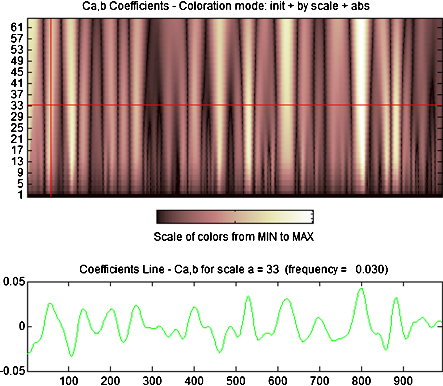
The coefficient under scale 33.

Given that different types of traces can select different scale coefficients as features, the coefficient is inversely proportional to the resolution. Smaller coefficient will have greater resolution, which is usually more representative of the overall trend. On the other hand, smaller coefficient with higher resolution has stronger noise interference, responding to local details rather than the overall trend. The characteristic should be the coefficient of moderate scale to remove the data of the lower-coefficient interval based on the following three points:

The data in the lower coefficient intervals have more details. These data should not be the characteristic because of the difference between the different traces, while the smaller scale components are usually the data of these individual differences as well as mechanical noise.

The data with higher scale are more suitable to describe the ups and downs of the surface traces and the smoothness after shearing, but the features of the tool are missing.

The algorithm aims at tracing the shear tool to maximize the commonality between traces and maintain tool trace differences. Therefore, the intermediate coefficient is more appropriate.

According to the detection device and actual experimental test, selecting the data near scale 35 is the most suitable choice.

The DTW algorithm is used to measure the similarity between the sample feature and the feature to be tested after the selection of the coefficient.

Set the sample to S ={ s₁, s₂, ⋯ , s_n } and the trace of the input to T ={ t₁, t₂, ⋯ , t_n }. Thus, a two-dimensional matrix A of size N * M can be constructed. The element a_(i,j) in the two-dimensional matrix represents the distance between the samples S ={ s₁, s₂, ⋯ , s_n } and the element j in I ={ i₁, i₂, ⋯ , i_m }.

Among Thus, the matrix a_(i,j) is calculated as follows: $a_{(i, j)} = e^{- {(s_{i} - t_{j})}^{2}}$ (8)

Equation (8) is a nonlinear equation. When the matching distance between the two is relatively close, its computational similarity can be kept at a high level where it tends to infinity when the distance exceeds a certain level. The similarity can be controlled in a lower range, and the distance similarity calculation does not appear inaccurate in this situation.

When the distance between s_i and t_j is the minimum, the highest degree of similarity is 1. As the distance increases, the degree of similarity becomes lower. The value can be infinitely close to 0. The DTW method is used to find the best matching path after obtaining the similarity degree between different points to obtain the maximum similarity value sims (n, m) at the end of the destination (n, m).

Figure 5 is the schematic diagram that finds the optimal matching after DTW calculation using two traces of the wavelet signature similarity matrix. In the diagram, vertical lines or horizontal lines represent the match for many times, while a slash indicates a new match.

Fig.5

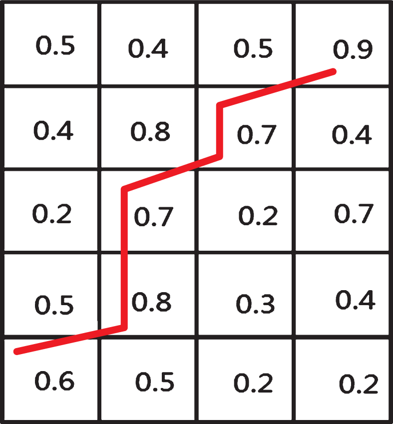
The schematic diagram of DTW matching.

The similarity of the dynamic programming equation is:

$dist (i, j) = min {\begin{matrix} dist (i - 1, j - 1) + d (A (i), B (j)) \\ dist (i - 1, j) + d (A (i), B (j)) \\ dist (i, j - 1) + d (A (i), B (j)) \end{matrix}$ (9)

The core idea of the dynamic local optimal method (greedy method) to give the new match a higher weight. In the DTW, whether the sample data at a certain position or input trace detection data at a certain position, has the same weight of the match of the first occurrence then it is given 1/2 or two, as long as it appears to match the other side of a number of locations. It can achieve the optimal matching when the condition of the two signal lengths is inconsistent.

As shown in Fig. 6, Data17 (blue) and Data18 (red) are repetitive detection signals of the same trace. The difference in the case of the smallest difference between the two data is shown in the third column. The two overlapped signal overlay is shown in the fourth column when the match is completed. Visual observation shows that the signal has a high degree of overlap. During the process of detection, some errors would inevitably be produced as the two cannot exactly be the same. The test results show that the similarity is 90%, which means that the two have been effectively aligned during matching.

Fig.6

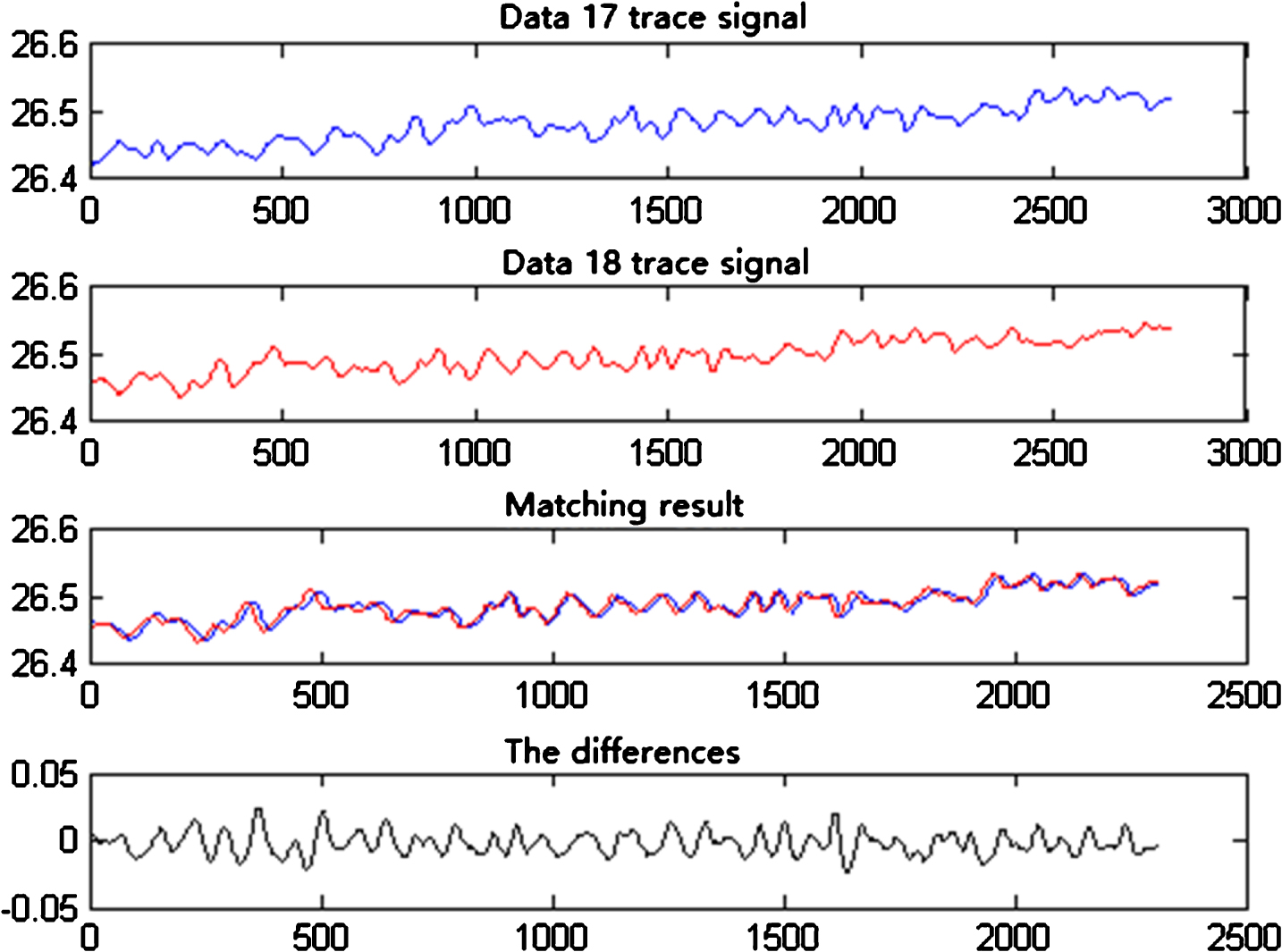
Signal difference matching.

The weight of the feature also affects the accuracy of recognition; therefore, performing specific parameter training can reduce the probability of failure. Parameter training involves the following basic steps:

Ensure that the steps complement the building of a sample library. The samples are sufficiently representative and distinguishable.

The gradient descent method is used for machine learning of parameters and constructing the corresponding cost function, reducing the costs of the cost function to a minimum by constant iterations [16, 17].

Completing the parameter training while acquiring learning parameters.

When the sample library changes or the scene of usage changes, a more targeted training is recommended to continue parameter training.

The sample trace detection signal gradient is used as an input, to calculate the degree of similarity, to identify corresponding groups of tools, to infer the possible attribution of the tool after calculation, and to obtain the degree of similarity of the data. The calculation of similarity needs to calculate the similarity degree between the sample and the input sample. The degree of similarity can be mapped to a range of 0 to 1. The minimum value of 0 represents completely different, while the maximum value of 1 represents exactly the same.

3.4. Sample library establishment

As the fundamental basis to identify the tools of trace signals, the quality of the sample library and the build mode directly affect the final result.

Its establishment usually follows the following steps:

Determine the types of tools, scope, and type that needed to identify. Each tool should be numbered by the uniform rules and the detailed parameter information should be recorded.

A single broken trace must be checked at least twice to eliminate the coincidence of detection. When the degree of coincidence between the two signal data points is more than 99%, the data can be regarded as qualified. The same broken trace is recommended to record different data at multiple locations, where each position should use the method given previously. The manual correction is allowed when necessary, as well as all means that are conducive to improve the quality and representation of the trace sample.

Using the data of this sample library as test data, each feature is tested at the same time after completing all the data collection. Test results show that the similarity of every sample data and their group data is significantly higher than other groups. If it is mixed together, the data are invalid, and then steps 1) and 2) are repeated.

3.5. Group identification

The comparison results of the data to be traced and all the samples in the library will be obtained after completing the similar calculation work. These results are the similar degree of a series of samples and input trace. Different types of tools and different locations of the shear will affect the results. Group identification is an effective tool that can aggregate such data and find the best possible data.

Group identification usually follows the following basic steps:

Sorting the similarity between the input trace data and the samples in the sample library. Usually, it can only sort the first 10% – 20% of the data.

Weighting the first 10% – 20% of the data. The weighted rule states that the higher the rank of the sequence, the greater the weight. Else, the data is assigned a low weight.

Grouping according to the weighting result, and calculating the size of the proportion of each group in the previous 10% – 20% data.

Sorting the data according to the proportion of each group and selecting the data sorted previously as the result of the derivation.

The entire process of tool traceability is shown below:

4. Experimental verification

The effectiveness of this algorithm is verified through the actual shear tool source experiment. The experimental set up is as follows:

Three tools were selected: wire cutters (A), destroy pliers (B), and steel wire clamp (C). A copper bar of 1 cm diameter was cut by shear breakage. All breakage surfaces were tested using the instrument described in the literature [2]. The sample parameter setting involved: a laser pot diameter of 2.5μm, a subdivided figure for 3200 steps/s, sample frequency pulse of 1000, sampling interval of 50 ms, sampling frequency of 20 Hz, the sampling points being determined according to the cross-sectional area of the broken end. The related algorithms that match the program were written in Python upon validatation by Matlab 2015b. The program was run on a ThinkPad laptop with Intel Core i5 2.9 GHz CPU with 8 G DDR3 memory.

The 29 sets of data labeled T16–T45 (T26 and T27 being substantially the same data) were used as test data. There were 500 data sets containing data on shearing by 10 different tools in the sample library. Excluding the data in the sample library, the results show the first five ranking values.

There were 3 sets of data in T16–T45. T16–T25 were from the traces formed by tool A, T26–T38 were from the traces formed by tools B1 and B2, and T39–T45 were from the traces formed by tool C. B1 and B2 are two tools that belong to the same tool B.

To make the simulation of the data collection in the crime scene more realistic, each group of test data was required to be tested again after shifting from the position based on the benchmark trace data and form the new data. The data in A mainly contained lateral displacement, that is the data moving on a straight line of the original traces. Some data coincided with the original data after the movement. At the same time, the data in A, B, and C, all had U-direction (up) and D-direction (down) movement and had a certain degree of dislocation with the original benchmark traces. The actual testing scenario is shown in Fig. 8.

Fig.7

Flowchart of tool tracing.

Fig.8

The actual test.

Table 1

The sample matching results by the algorithm proposed in this study

Tool number	Highest matching	Accurate traceability rate	Data description
T16	T17	100%	Group A benchmark data
T17	T16	100%	Group A benchmark data duplicate detection
T18	T20	100%	Group A benchmark data displacement 1/6
T19	T20	100%	Group A benchmark data displacement 1/3
T20	T21	100%	Group A benchmark data displacement 1/3
T21	T20	100%	Group A benchmark data displacement 1/2
T22	T23	100%	With the end of broken A another line
T23	T18	100%	T22 based on the direction D of translation of 1/6 of the other line
T24	T39	40%	T22 based on the direction U of translation of 1/6 of the other line
T25	T41	40%	Dislocation 1/3 and deletion of 2/3 based on T22
T26	T27	100%	Group B benchmark data
T27	T26	100%	Group B benchmark data duplicate detection
T28	T27	100%	Group B benchmark data duplicate detection
T29	T30	100%	Group B based on the direction D of translation of 1/10 of the other line
T30	T29	100%	T29 duplicate detection
T31	T32	100%	Group B based on the direction U of translation of 1/10 of the other line
T32	T31	100%	T31 duplicate detection
T33	T34	100%	Group B similar tools, different ends
T34	T33	100%	T33 duplicate detection
T35	T36	100%	T33 based on the direction D of translation of 1/10 of the other line
T36	T35	100%	T35 duplicate detection
T37	T38	80%	T35based on the direction D of translation of 1/10 of the other line
T38	T37	80%	T38 duplicate detection
T39	T40	80%	Group C benchmark data
T40	T39	80%	Group C benchmark data duplicate detection
T41	T25	60%	Group C based on the direction D of translation of 1/10 of the other line
T42	T43	80%	T41 duplicate detection
T43	T42	80%	T41 duplicate detection
T44	T45	80%	Group C based on the direction U of translation of 1/10 of the other line
T45	T44	80%	T44 duplicate detection

The definitions of tool traceability are as follows:

Backtrack precisely for the same trace (or tool). There is a certain deviation because of the location of detection, the length of the data, and many others. The sorting is more on the front and it has differentiated between the similarity degree of other types of tools.

Backtrack failed: Data not associated with the original trace.

The calculation takes 15 s, with an 88.9% matching success rate and 11.1% failure rate.

To draw a comparison with the technology proposed in this study, the literature [8] algorithm is used for a total of 145 tests using the same 29 sets of data labled T16–T45. The results are shown in Table 2.

Table 2

The sample matching results by the algorithm proposed in reference [8]

Tool number	Highest matching	Accurate traceability rate	Data description
T16	T18	80%	Group A benchmark data
T17	T16	60%	Group A benchmark data duplicate detection
T18	else	20%	Group A benchmark data displacement 1/6
T19	else	20%	Group A benchmark data displacement 1/3
T20	else	20%	Group A benchmark data displacement 1/3
T21	T16	60%	Group A benchmark data displacement 1/2
T22	T23	60%	With the end of broken A another line
T23	T22	80%	T22 based on the direction D of translation of 1/6 of the other line
T24	else	0%	T22 based on the direction U of translation of 1/6 of the other line
T25	else	0%	Dislocation 1/3 and deletion of 2/3 based on T22
T26	T27	80%	Group B benchmark data
T27	T26	80%	Group B benchmark data duplicate detection
T28	T27	80%	Group B benchmark data duplicate detection
T29	T26	60%	Group B based on the direction D of translation of 1/10 of the other line
T30	T26	60%	T29 duplicate detection
T31	else	0%	Group B based on the direction U of translation of 1/10 of the other line
T32	T31	100%	T31 duplicate detection
T33	T34	60%	Group B similar tools, different ends
T34	T33	60%	T33 duplicate detection
T35	T37	20%	T33 based on the direction D of translation of 1/10 of the other line
T36	else	0%	T35 duplicate detection
T37	else	0%	T35based on the direction D of translation of 1/10 of the other line
T38	T37	60%	T38 duplicate detection
T39	T40	80%	Group C benchmark data
T40	T39	80%	Group C benchmark data duplicate detection
T41	T25	20%	Group C based on the direction D of translation of 1/10 of the other line
T42	T43	60%	T41 duplicate detection
T43	T42	60%	T41 duplicate detection
T44	T45	60%	Group C based on the direction U of translation of 1/10 of the other line
T45	T44	60%	T44 duplicate detection

Table 2. The sample matching results by the algorithm proposed in reference [8].

The calculation takes 18 s, with a matching success rate at 51%, the failure rate at 49%.

Compared to the method proposed in literature [8], the traceability technique of proposed in this study has obvious advantages in the operation precision and stability order. Although there are no obvious differences in the speed of operation, the proposed method is more applicable to test the traces data in actual scene detection.

5. Summary and prospect

In this study, a fast traceability algorithm for non-linear shear traces in the wavelet domain was proposed. The proposed algorithm combines the dynamic time regularization algorithm based on wavelet features to perform similarity matching of trace features and realize the rapid inference of corresponding tools. The complexity of the algorithm presented in this study is relatively low. The algorithm can be programmed directly using the Python language, and the generated executable file can be run on mid-range computers. Through actual tests by an expert from the trace testing works in the Ministry of Public Security, the algorithm is proved to be effectively applicable to the shear tools backtrack based on line trace and provide a reliable reference for subsequent identification. To simulate actual working environments more realistically, improve the operation speed of larger magnitude data, and perform comparative and traceability studies of serial criminal offenders in the cross-region faster are avenues for future research.

Footnotes

Acknowledgments

This article was supported by the key project of technology research program funded by Yunnan Province (approved grants 2016RA042), the Innovation Fund for Technology based firms in Yunnan Province (approved grants 2014SC030 and 2017EH028), the key science and technology project of Kunming City (approved grants 2015-1-S-00284), the Ministry of public security technology research program (approved grants 2014JSYJA020 and 2016JSYJA03), and the international cooperation training program for innovative talents funded by China Scholarship Council (approved grants 201608740005).

References

Bunch and

Wevers , Application of likelihood ratios for firearm and toolmark analysis, Science and Justice 53(2) (2013), 223–229.

Liu ,

Pan ,

Sha , et al., One police laser detection system for linear traces, China Patent, CN 105300996 A, 2016, 02, 03. (in Chinese)

Gambino ,

Mclaughlin ,

Kuo , et al., Forensic surface metrology: Tool mark evidence, Scanning 33(5) (2011), 272–278.

Baiker ,

Keereweer ,

Pieterman , et.al., Quantitative comparison of striated toolmarks, Forensic Science International 242 (2014), 186–199.

Kassamakov ,

Barbeau ,

Lehto , et al., CSI Helsinki: Comparing three-dimensional imaging of diagonal cutter toolmarks using confocal microscopy and SWLI, Three-Dimensional Imaging, Visualization, and Display 2010 and Display Technologies and Applications for Defense, Security, and Avionics IV, Orlando, FL, United States, 2010, 7690:76900Y.

Yang ,

D.Y.

Li and

W.D.

Wang , The study of tool mark identification based on local wavelet energy, Journal of People's Public Security University of China(Science and Technology) 56 (2008), 73–75.

B.C.

Wang ,

Z.H.

Ren ,

L.Y.

Ren , et al., Fractal geometry description of the surface appearance of the shearing trace, Machinery Design & Manufacture 160 (2003), 106–107.

Pan ,

Wu ,

Liu , et al., Research on the adaptive matching algorithm for laser linear mark detection signals, Chinese Journal of Scientific Instrument 36(6) (2015), 1372–1380.

H.L.

Cui ,

Liu ,

Yu , et al., Application of wavelet denoising in distributed optical fiber interferometric vibration detection and location system, Optics and Precision Engineering 23 (2015), 71–76.

10.

S.L.

Ye ,

Y.D.

Zhang and

Zhang , Scale and directional correlation combined denoiseing in gear visual inspection, Optics and Precision Engineering 22(6) (2014), 1622–1630.

11.

M.Z.

Zhang ,

J.H.

Mou ,

Liu , et al., Phase extraction for fringe patterns based on complex Morlet wavelet transform, Optics and Precision Engineering 20(3) (2012), 643–650.

12.

Ogawa ,

Sakata and

Li , Adaptive noise reduction of scintigrams with a wavelet transform, Hindawi Publishing Corporation 2012(11) (2011), 130482.

13.

Zheng ,

L.M.

Xiao ,

W.Q.

Tang , et al., Parallelization of dynamic time warping on a heterogeneous platform, Maruzen Co, Ltd E97A(11) (2014), 2258–2262.

14.

H.L.

Li , On-line and dynamic time warping for time series data mining, Springer Verlag 6 (2014), 145–153.

15.

Dupas ,

Tavenard and

Ophelie , Identifying seasonal patterns of phosphorus storm dynamics with dynamic time warping, Blackwell Publishing Ltd 51 (2015), 8868–8882.

16.

Jia and

E.Y.

Lam , Machine learning for inverse lithography: Using stochastic gradient descent for robust photomask synthesis, Institute of Physics Publishing 12(4) (2010), 45601–45609.

17.

Shao and

J.Y.

Yang , Multi-robot reinforcement learning based on learning classifier system with gradient descent methods, Binary Information Press 6 (2010), 2449–2455.