A heuristic approach to bicycle repositioning problems with dynamic pricing

Abstract

Bicycle-sharing systems are commonly established at geographically dispersed locations to create their rental service networks. To provide customers with flexibility and convenience, bicycle-sharing systems commonly allow them to pick up bicycles from one station and return them to a different one. However, allowing customers to return their rented bicycles to different stations can possibly lead to an imbalance in the bicycle rental network. One of the approaches to overcome the bicycle imbalance problem is to apply dynamic pricing to motivate consumers to return the rented bicycles to stations without a sufficient number of bicycles. This study developed a constrained dynamic pricing model to address the bicycle imbalance problem. Moreover, this study aimed to maximize the total revenues over a planning horizon through dynamic pricing strategies. We identify some necessary conditions for optimal sale prices. Using these conditions, we develop a heuristic algorithm based on linear programming and an evolutionary algorithm to efficiently produce comprise solutions. The proposed model and solution procedure were applied to analyze the bicycle system in Taiwan. Sensitivity analyses were also conducted to investigate the effects of various system parameters.

Keywords

Bicycle sharing rental network imbalance dynamic pricing algorithm

1. Introduction

The reasons for people’s preference for bicycles as their transportation mode vary considerably [16]. With regard to public policy, cycling is considered a sustainable transport mode, which decreases greenhouse gases as well as noise and air pollutions given that considerably few people travel by car. Cycling also decreases traffic congestion and the potential risk of traffic accidents and fatalities. For private individuals, cycling benefits include increased physical activity levels, increased opportunity to spend quality time with friends and family, and decreased traffic congestion when moving around urban areas. In addition, cycling can solve the last mile problem for users who seek connections to public transit networks.

The increasing popularity of cycling has encouraged several organizations to join the bicycle rental business. To increase market share and competitiveness, many bicycle rental companies establish multiple rental branches at geographically dispersed locations to create their bicycle rental networks. Leveraging their rental networks, these companies allow customers to pick up bicycles from one station and return them to a different one. This service model provides customers flexibility and convenience and can enhance the competitiveness of the rental company. However, allowing customers to return their rented bicycles to different stations can possibly lead to an imbalance in the bicycle rental network. Specifically, stations with low demands will probably accumulate a surplus of idle bicycles, whereas stations with high demands will possibly experience a bicycle shortage [25]. The potential imbalance of supply and demand at the bicycle stations can probably result in lost sales at stations experiencing relatively high demands and under-utilization of assets at stations experiencing relatively low demands.

Bicycle firms can overcome the imbalance problem using the supply or the demand management approaches to improve service quality or profits. Supply management approaches mainly aim to rebalance the bicycle system through bicycle repositioning planning that balances the available supply with anticipated demands. The repositioning planning problem includes the resource deployment problem, which determines fleet levels for all branches, and the transportation operation problem, which anticipates the required resource transfers among branches. Over the years, several works related to bicycle and car rental problems have proposed mathematical models to deal with transfer planning problems. These studies aimed to focus on minimizing travel costs and times ([2, 4]), minimizing unsatisfied demands ([13 , 21]) or minimizing both of them ([6 , 27]). The mathematical models in the literature are established in terms of linear programming models ([1, 23]), integer or dynamic programming models ([8–10 , 26]) and queuing models ([11 , 22]).

The repositioning problem is generally considered non-deterministic polynomial-time (NP)-hard; thus, many researchers applied meta-heuristic algorithms or develop heuristics to solve their proposed models ([15 , 29]). These approaches are not guaranteed to produce the exact optimum solutions. However, they can produce compromise solutions or acceptable optimums within reasonable computational times. Accordingly, when problems have substantial computational complexities and are computationally intractable (such as NP-hard problems), these approaches are usually considered given that accurately solving such type of problems can take an exponential amount of computation time [24]. Yaghini and Khandaghabadi [29] developed a genetic algorithm and simulated annealing-based algorithms to deal with a dynamic fleet-sizing problem. Sayarshad and Ghoseiri [23] applied the simulated annealing approach to deal with a railcar fleet-sizing problem. Oliveira et al. [15] presented a relax-and-fix-based algorithm to study a vehicle-reservation assignment problem.

Several researchers have dealt with the repositioning problem in terms of supply management approaches ([7 , 30]). In addition to supply management methods, demand management approaches can be used to balance demand and supply. However, to the best of our knowledge, few researchers have attempted to overcome the problem using the demand management approaches. The application of price discounts has been viewed by many industries as one of the effective demand management tools to balance demand and supply. For example, in the car rental industry, Hertz offers 10% to 30% car rental discounts during different seasons. In general, high price discounts result in high demand levels. On the contrary, low price discounts or price surcharges result in low demand levels. Therefore, rental companies should view their pricing strategies as a revenue enhancement tool and as a key weapon to address the demand management problem.

Problems associated with pricing planning for service capacity are discussed primarily in the study of revenue management. However, the application of revenue management to the control of perishable capacity mainly focuses on whether to accept or reject incoming booking reservations ([3 , 28]) and rarely discuss the pricing and balancing problem of bicycle-sharing systems. Consequently, the literature currently lacks a model that can simultaneously consider the decisions related to the determination of rental prices for the closed rental bicycle system. This study developed a constrained mathematical model, which uses dynamic pricing to balance the bicycle status across the bicycle stations. We aim to maximize the total profit over a planning horizon through dynamic pricing. We find some necessary conditions for sale prices to be the extreme points of the objective function. Using these conditions, we develop a heuristic algorithm, which is based on linear programming, and an evolutionary algorithm to solve the proposed model. The proposed model and solution procedure were applied to the analysis of actual cases in Taiwan. Sensitivity analyses were also conducted to investigate the effects of various system parameters.

2. Model description and Formulation

A bicycle rental company aims to create a pricing plan for its rental business over M branches in T planning periods. D_i docking poles are available at Branch i, and at all branches, and the minimum and maximum durations are one and K rental periods, respectively. We suppose that the number of bicycles initially allocated at Branch i at the start of period-1 is v_1i and that no bicycle is on lease at the start of period-1. The fleet size of the bicycles, S, is the sum of bicycles allocated at all branches at the start of the planning horizon. Therefore, $S = \sum_{i = 1}^{M} v_{1 i}$ . The value of S remained constant over the planning periods. During the rental process, the inventory level at each branch at the start of the following subsequent period is influenced by the number of bicycles on lease and of returned ones.

The company allows customers to pick up bicycles from one station and return them to a different one. To distinguish the different request types, we use symbols (t, i, j, k) to denote the rental type for k periods at the start of period t at Branch i and the bicycle return to Branch j at the end of period t + k - 1. The number of rental requests for each rental type (t, i, j, k) is assumed to be price dependent and follows a known deterministic function d_tijk (p), where d_tijk (p) is a non-increasing function and d_tijk (p) p is a concave function of sale price-p. In each period, the company determines the price to be set for each rental type. On each planning period, the company operates the rental business through determining rental prices to control the inventory level of bicycles at each branch. The minimum sale price for the k rental periods is assumed to be $p_{k}^{\min}$ .

For each period, we assume that the sequence of events proceeds as follows: rental requests and then bicycle returns. In each period, the company first decides the rental prices for all branches. The company can predict the number of rental requests that will be made based on the relationship between price and rental requests. All customers are assumed to return their rented bicycles to their destination branches at the end of the due period.

The following parameters and variables are used to develop our model.

Notation:

[K:] maximum number of rental periods,

[M:] number of branches,

[T:] number of planning periods,

[S:] total number of bikes,

[(t, i, j, k):] a demand for renting a bicycle at Branch-i at the start of period-t and returning the object at Branch-j at the end of period-t+k-1,

[D_ij:] number of docking poles at Branch-i,

[d_tijk (p):] requests for rental type (t, i, j, k) when the sales price is set at p,

[ $p_{k}^{\min}$ :] lowest rental fee for k rental periods,

[S:] fleet size.

[v_ti:] number of bicycle available at Branch-i at the start of period t,

[p_tijk:] rental fee for rental type (t, i, j, k).

The purpose is to maximize the total profit over T operational periods through determining p_tijk and v_ti.

For Branch-i in period t, when price p_tijk is offered for rental type (t, i, j, k), d_tijk (p_tijk) units of rental requests are rented out. Below, we use symbol x_tijk to stand for d_tijk (p_tijk). In this case, the revenue from rental type (t, i, j, k) is x_tijkp_tijk. Let PR denote the total expected revenues over all planning periods. Thereafter, we can express PR as Eq.(1).

$PR = \sum_{t = 1}^{T} \sum_{i = 1}^{M} \sum_{j = 1}^{M} \sum_{k = 1}^{K} x_{tijk} p_{ijk}^{n} .$ (1)

Bicycle capacity, S, remained constant over all periods. For t ≥ 2, all bicycles may not necessarily be stocked in the company branches given that some of them are on lease. The total bicycle inventory includes the sum of bicycles available at all branches at the start of the period and the ones on lease. For period t ≥ 2 and the maximum rental period K = 1, given that all bicycles are returned in the same period, the sum of the bicycles remaining at all branches at the start of a period should be equal to the fleet size, S. Therefore, for K = 1, we have constraint (2).

$\sum_{i = 1}^{M} v_{ti} = S, \forall t > 1 or K = 1 .$ (2)

For period t ≥ 2 and the maximum rental period K > 1, the number of bicycles available at all branches at the start of the period is $\sum_{i = 1}^{M} v_{ti}$ . Suppose that a bicycle is rented out at t - k ≥ 1 (k periods before period t) with rental duration g periods. According to the modeling assumption, the bicycle is still on lease at the start of period-t if the rental duration is g > k. Therefore, the number of bicycles on lease at the start of period t ≥ 2 is $\sum_{i = 1}^{M} \sum_{j = 1}^{M} \sum_{k = 1}^{t - 1} \sum_{g = k + 1}^{K} x_{t - k, ijg}$ for 2 ≤ t ≤ K and $\sum_{i = 1}^{M} \sum_{j = 1}^{M} \sum_{k = 1}^{K - 1} \sum_{g = k + 1}^{K} x_{t - k, ijg}$ for 2 ≤ K < t. The fleet size remained constant over all subsequent periods; thus, we have constraint (3).

$\begin{matrix} \sum_{i = 1}^{M} v_{ti} + \sum_{i = 1}^{M} \sum_{j = 1}^{M} \sum_{k = 1}^{min {t - 1, K - 1}} \sum_{g = k + 1}^{K} x_{t - k, ijg} = S, \\ \forall t \geq 2 . \end{matrix}$ (3)

The total number of bicycles stocked at a station cannot exceed its total docking poles. Accordingly, we have constraint (4).

$v_{ti} \leq D_{i} . \forall t, i .$ (4)

The number of bicycles to be leased out at any branch at any period cannot exceed the available bicycles at the branch; thus, we require constraint (5).

$\sum_{j = 1}^{M} \sum_{k = 1}^{K} x_{tijk} \leq v_{ti}, \forall t, i .$ (5)

Bicycles available in the morning of period t at Branch i, v_ti, minus the number of bicycles rented plus the number of returned ones is level v_t+1,i. Hence, v_ti and v_t+1,i have the following relationship.

$\begin{matrix} v_{t + 1, i} = v_{ti} - \sum_{j = 1}^{M} \sum_{k = 1}^{K} x_{tijk} \\ + \sum_{j = 1}^{M} \sum_{k = 1}^{min {K, t}} x_{t - k + 1, jik}, \forall t < T, i . \end{matrix}$ (6)

Rental fee for k-rental periods cannot be lower than $p_{k}^{\min}$ . Therefore, we have constraint (7).

$p_{tijk} \geq p_{k}^{\min}, \forall t, i, j, k .$ (7)

The purpose is to maximize the profit of the firm over T operational periods through determining decisions p_tijk, v_ti and x_tijk. We refer to the mathematical model in the form of maximizing the PR subject to constraints (2)-(7) as Model-1.

3. Metholodgy

3.1. Modeling Analysis

In model M1, the unknown decision variables include p_tijk, v_ti, and dependent variables x_tijk. To reduce the number of variables, we will express the recursive function v_ti in terms of the known parameter v_1i and decision variable x_tijk.

Lemma 1: v_ti can be re-expressed by (8) and (9).

$\begin{matrix} v_{ti} = v_{1 i} - \sum_{s = 1}^{t - 1} \sum_{j = 1}^{M} \sum_{k = 1}^{K} x_{sijk} \\ + \sum_{s = 1}^{t - 1} \sum_{j = 1}^{M} \sum_{k = 1}^{t - s} x_{sjik}, \forall i, 1 < t \leq K . \end{matrix}$ (8) $\begin{matrix} v_{ti} = v_{1 i} - \sum_{s = 1}^{t - 1} \sum_{j = 1}^{M} \sum_{k = 1}^{K} x_{sijk} + \sum_{s = 1}^{t - K} \sum_{j = 1}^{M} \sum_{k = 1}^{K} x_{sjik} \\ + \sum_{s = t - K + 1}^{t - 1} \sum_{j = 1}^{M} \sum_{k = 1}^{t - s} x_{sjik}, \forall i, 1 < K < t . \end{matrix}$ (9)

Proof: The assertion holds for t = 2 and t ≤ K since from (6) we have

$v_{2 i} = v_{1 i} - \sum_{s = 1}^{1} \sum_{j = 1}^{M} (\sum_{k = 1}^{K} x_{sijk} - \sum_{k = 1}^{1} x_{sjik}), \forall i .$ (10)

Assume the assertion holds for t - 1, we have

$\begin{matrix} v_{ti} = v_{t - 1, i} - \sum_{j = 1}^{M} \sum_{k = 1}^{K} x_{t - 1, ijk} + \sum_{j = 1}^{M} \sum_{k = 1}^{t - 1} x_{t - k, jik} \\ = v_{1 i} - \sum_{s = 1}^{t - 2} \sum_{j = 1}^{M} \sum_{k = 1}^{K} x_{sijk} + \sum_{s = 1}^{t - 2} \sum_{j = 1}^{M} \sum_{k = 1}^{t - 1 - s} x_{sijk} \\ - \sum_{j = 1}^{M} \sum_{k = 1}^{K} x_{t - 1, ijk} + \sum_{j = 1}^{M} \sum_{k = 1}^{t - 1} x_{t - k, jik} \\ = v_{1 i} - \sum_{s = 1}^{t - 1} \sum_{j = 1}^{M} (\sum_{k = 1}^{K} x_{sijk} - \sum_{k = 1}^{t - 2} x_{sjik}) . \end{matrix}$ (11)

Thus, the assertion of equation (8) holds. For t = K + 1, By (6) and (8), we have

$\begin{matrix} v_{K + 1, i} \\ = & v_{Ki} - \sum_{j = 1}^{M} \sum_{k = 1}^{K} x_{Kijk} + \sum_{j = 1}^{M} \sum_{k = 1}^{K} x_{K - k + 1, jik} \\ = & v_{1 i} - \sum_{s = 1}^{K - 1} \sum_{j = 1}^{M} \sum_{k = 1}^{K} x_{sijk} + \sum_{s = 1}^{K - 1} \sum_{j = 1}^{M} \sum_{k = 1}^{K - s} x_{sijk} \\ - \sum_{j = 1}^{M} \sum_{k = 1}^{K} x_{Kijk} + \sum_{j = 1}^{M} \sum_{k = 1}^{t - 1} x_{K - k + 1, jik} \\ = & v_{1 i} - \sum_{s = 1}^{K} \sum_{j = 1}^{M} \sum_{k = 1}^{K} x_{sijk} + \sum_{s = 1}^{1} \sum_{j = 1}^{M} \sum_{k = 1}^{K} x_{sjik} \\ + \sum_{s = 2}^{K} \sum_{j = 1}^{M} \sum_{k = 1}^{K - s + 1} x_{sjik} . \end{matrix}$ (12)

Thus, the assertion of Eq.(9) holds for t = K + 1. Using the same logic, by induction, we can show that

$\begin{matrix} v_{ti} & = & v_{1 i} - \sum_{s = 1}^{t - 2} \sum_{j = 1}^{M} \sum_{k = 1}^{K} x_{sijk} + \sum_{s = 1}^{t - K - 1} \sum_{j = 1}^{M} \sum_{k = 1}^{K} x_{sjik} \\ + \sum_{s = t - K}^{t - 2} \sum_{j = 1}^{M} \sum_{k = 1}^{t - s - 1} x_{sjik} - \sum_{j = 1}^{M} \sum_{k = 1}^{K} x_{t - 1, ijk} \\ + \sum_{j = 1}^{M} \sum_{k = 1}^{K} x_{t - k, jik} \end{matrix}$

$\begin{matrix} = & v_{1 i} - \sum_{s = 1}^{t - 1} \sum_{j = 1}^{M} \sum_{k = 1}^{K} x_{sijk} + \sum_{s = 1}^{t - K} \sum_{j = 1}^{M} \sum_{k = 1}^{K} x_{sjik} \\ + \sum_{s = t - K + 1}^{t - 1} \sum_{j = 1}^{M} \sum_{k = 1}^{t - s} x_{sjik} . \end{matrix}$ (13)

Thus, we have completed the proof of Lemma 1.

Lemma 2: Setting v_ti as that in constraints (8) and (9) is equivalent to setting constraint (3).

Proof: For 2 ≤ t ≤ K, substituting equation (8) into constraint (3), we have

$\begin{matrix} \sum_{i = 1}^{M} v_{1 i} - \sum_{s = 1}^{t - 1} \sum_{i = 1}^{M} \sum_{j = 1}^{M} \sum_{k = 1}^{K} x_{sijk} \\ + \sum_{s = 1}^{t - 1} \sum_{i = 1}^{M} \sum_{j = 1}^{M} \sum_{k = 1}^{t - s} x_{sjik} \\ + \sum_{i = 1}^{M} \sum_{j = 1}^{M} \sum_{k = 1}^{t - 1} \sum_{g = k + 1}^{K} x_{t - k, ijg} = S . \end{matrix}$ (14)

Since $\sum_{i = 1}^{M} \sum_{j = 1}^{M} \sum_{k = 1}^{t - 1} \sum_{g = k + 1}^{K} x_{t - k, ijg} =$ $\sum_{s = 1}^{t - 1}$ $\sum_{i = 1}^{M} \sum_{j = 1}^{M} \sum_{k = t - s + 1}^{K} x_{sijk}$ , we have

$\begin{matrix} \sum_{s = 1}^{t - 1} \sum_{i = 1}^{M} \sum_{j = 1}^{M} \sum_{k = 1}^{t - s} x_{sjik} + \sum_{s = 1}^{t - 1} \sum_{i = 1}^{M} \sum_{j = 1}^{M} \sum_{k = 1}^{K} x_{t - k, ijg} \\ = \sum_{s = 1}^{t - 1} \sum_{i = 1}^{M} \sum_{j = 1}^{M} \sum_{k = 1}^{K} x_{sijk} . \end{matrix}$ (15)

Thus, the right-hand side of Eq. (14) becomes $\sum_{i = 1}^{M} v_{1 i}$ . the result of $\sum_{i = 1}^{M} v_{1 i}$ is the total capacity, that is $\sum_{i = 1}^{M} v_{1 i} = S$ , and thus the statement holds for 2 ≤ t ≤ K. For 2 ≤ K < t, substituting equation (9) in constraint (3), we have

$\begin{matrix} \sum_{i = 1}^{M} v_{1 i} - \sum_{s = 1}^{t - 1} \sum_{i = 1}^{M} \sum_{j = 1}^{M} \sum_{k = 1}^{K} x_{sijk} \\ + \sum_{s = 1}^{t - K} \sum_{i = 1}^{M} \sum_{j = 1}^{M} \sum_{k = 1}^{K} x_{sjik} \\ + \sum_{s = t - K + 1}^{t - 1} \sum_{i = 1}^{M} \sum_{j = 1}^{M} \sum_{k = 1}^{t - s} x_{sjik} \\ + \sum_{i = 1}^{M} \sum_{j = 1}^{M} \sum_{k = 1}^{K - 1} \sum_{g = k + 1}^{K} x_{t - k, ijg} = S . \end{matrix}$ (16)

Note

$\begin{matrix} \sum_{i = 1}^{M} \sum_{j = 1}^{M} \sum_{k = 1}^{K - 1} \sum_{g = k + 1}^{K} x_{t - k, ijg} \\ = \sum_{s = t - K + 1}^{t - 1} \sum_{i = 1}^{M} \sum_{j = 1}^{M} \sum_{k = t - s + 1}^{K} x_{sijk} . \end{matrix}$ (17)

Then, it is clear that the sum of second, third, fourth and fifth terms is zero. The remining term in the right hand side of (3) is $\sum_{i = 1}^{M} v_{1 i}$ . Thus, the right-hand side of (3) eventually leads to $\sum_{i = 1}^{M} v_{1 i} = S$ when v_ti is set by (8) and (9) and the result follows.

Substituting constraints (8) and (9) in constraint (4), we can express constraint (4) by constraints (18), (19) and constraint (5) by constraints (20) to (22).

$\begin{matrix} v_{1 i} - \sum_{s = 1}^{t - 1} \sum_{j = 1}^{M} \sum_{k = 1}^{K} x_{sijk} + \sum_{s = 1}^{t - 1} \sum_{j = 1}^{M} \sum_{k = 1}^{t - s} x_{sjik} \\ \leq D_{i}, \forall 2 \leq t \leq K, i, \end{matrix}$ (18) $\begin{matrix} v_{1 i} - \sum_{s = 1}^{t - 1} \sum_{j = 1}^{M} \sum_{k = 1}^{K} x_{sijk} + \sum_{s = 1}^{t - K} \sum_{j = 1}^{M} \sum_{k = 1}^{K} x_{sjik} \\ + \sum_{s = t - K + 1}^{t - 1} \sum_{j = 1}^{M} \sum_{k = 1}^{t - s} x_{sjik} \leq D_{i}, \\ \forall 2 \leq K < t, i, \end{matrix}$ (19) $\sum_{j = 1}^{M} \sum_{k = 1}^{K} x_{1 ijk} - v_{1 i} \leq 0, \forall i,$ (20) $\begin{matrix} \sum_{j = 1}^{M} \sum_{k = 1}^{K} x_{tijk} - v_{1 i} + \sum_{s = 1}^{t - 1} \sum_{j = 1}^{M} \sum_{k = 1}^{K} x_{sijk} \\ - \sum_{s = 1}^{t - 1} \sum_{j = 1}^{M} \sum_{k = 1}^{t - s} x_{sjik} \leq 0, \forall 2 \leq t \leq K, i, \end{matrix}$ (21) $\begin{matrix} \sum_{j = 1}^{M} \sum_{k = 1}^{K} x_{tijk} - v_{1 i} + \sum_{s = 1}^{t - 1} \sum_{j = 1}^{M} \sum_{k = 1}^{K} x_{sijk} \\ - \sum_{s = 1}^{t - K} \sum_{j = 1}^{M} \sum_{k = 1}^{K} x_{sjik} - \sum_{s = t - K + 1}^{t - 1} \sum_{j = 1}^{M} \sum_{k = 1}^{t - s} x_{sjik} \\ \leq 0, \forall 2 \leq K < t, i, \end{matrix}$ (22)

Combining equations (18)-(22) and Lemma 2, we can reduce variable v_ti in Model-1 and can re-express Model-1 as the form of maximizing PR subject to constraints (7) and (18-22). We refer to this model as Model-2 and show Model-2’s Lagrangean function below.

Lagrangean function:

The Lagrangean function of the problem L (P) is given as follows.

$L (P) = PR - L_{1} - L_{2} - L 3$ (23)

where

$\begin{matrix} L_{1} = \sum_{t = 2}^{K} \sum_{i = 1}^{M} λ_{ti} (v_{1 i} - \sum_{s = 1}^{t - 1} \sum_{j = 1}^{M} \sum_{k = 1}^{K} x_{sijk} \\ + \sum_{s = 1}^{t - 1} \sum_{j = 1}^{M} \sum_{k = 1}^{t - s} x_{sjik} - D_{i} + μ_{ti}^{2}) \\ + \sum_{t = K + 1}^{T} \sum_{i = 1}^{M} λ_{ti} (v_{1 i} - \sum_{s = t - K + 1}^{t - 1} \sum_{j = 1}^{M} \sum_{k = 1}^{K} x_{sijk} \\ + \sum_{s = t - K + 1}^{t - 1} \sum_{j = 1}^{M} \sum_{k = 1}^{t - s} x_{sjik} - D_{i} + μ_{ti}^{2}), \end{matrix}$ (24) $\begin{matrix} L_{2} = \sum_{i = 1}^{M} γ_{1 i} (\sum_{j = 1}^{M} \sum_{k = 1}^{K} x_{1 ijk} - v_{1 i} + w_{1 i}^{2}) \\ - \sum_{t = 2}^{K} \sum_{i = 1}^{M} γ_{ti} (\sum_{j = 1}^{M} \sum_{k = 1}^{K} x_{1 ijk} - v_{1 i} \\ + \sum_{s = 1}^{t - 1} \sum_{j = 1}^{M} \sum_{k = 1}^{K} x_{sijk} - \sum_{s = 1}^{t - 1} \sum_{j = 1}^{M} \sum_{k = 1}^{t - s} x_{sjik} + w_{ti}^{2}) \\ + \sum_{t = K + 1}^{T} \sum_{i = 1}^{M} γ_{ti} (\sum_{j = 1}^{M} \sum_{k = 1}^{K} x_{tijk} - v_{1 i} \\ + \sum_{s = 1}^{t - 1} \sum_{j = 1}^{M} \sum_{k = 1}^{K} x_{sijk} - \sum_{s = 1}^{t - K} \sum_{j = 1}^{M} \sum_{k = 1}^{K} x_{sjik} \\ - \sum_{s = t - K + 1}^{t - 1} \sum_{j = 1}^{M} \sum_{k = 1}^{t - s} x_{sjik} + w_{ti}^{2}) . \end{matrix}$ (25) $L_{3} = \sum_{t = 1}^{T} \sum_{i = 1}^{M} \sum_{j = 1}^{M} η_{tijk} \sum_{k = 1}^{K} (p_{k}^{\min} - p_{tijk} + h_{tijk}^{2}) .$ (26)

where λ_ti, γ_ti and η_tijk are the Lagrange multiplier associated with the above constraints.

Remark 1: L₁ and L₂ can be rearranged as (27) and (28), respectively.

$\begin{matrix} L_{1} = - \sum_{t = 1}^{K - 1} \sum_{i = 1}^{M} \sum_{j = 1}^{M} \sum_{k = 1}^{K} x_{tijk} \sum_{s = t + 1}^{K} λ_{si} \\ + \sum_{t = 1}^{K - 1} \sum_{i = 1}^{M} \sum_{j = 1}^{M} \sum_{k = 1}^{K - t + 1} x_{tijk} \sum_{s = t + k}^{K} λ_{sj} \\ - \sum_{t = 2}^{K} \sum_{i = 1}^{M} \sum_{j = 1}^{M} \sum_{k = 1}^{K} x_{tijk} \sum_{s = K + 1}^{K + t - 1} λ_{si} \\ - \sum_{t = K + 1}^{T - K} \sum_{i = 1}^{M} \sum_{j = 1}^{M} \sum_{k = 1}^{K} x_{tijk} \sum_{s = t + 1}^{K + t - 1} λ_{si} \\ - \sum_{t = T - K + 1}^{T - 1} \sum_{i = 1}^{M} \sum_{j = 1}^{M} \sum_{k = 1}^{K} x_{tijk} \sum_{s = t + 1}^{T} λ_{si} \\ + \sum_{t = 2}^{T} \sum_{i = 1}^{M} λ_{ti} (v_{1 i} - D_{i} + μ_{ti}^{2}) \\ + \sum_{t = K + 1}^{T} \sum_{s = t - K + 1}^{t - 1} \sum_{i = 1}^{M} \sum_{j = 1}^{M} \sum_{k = 1}^{t - s} x_{sijk} λ_{sj} . \end{matrix}$ (27)

$\begin{matrix} L_{2} = \sum_{t = 1}^{T} \sum_{i = 1}^{M} \sum_{j = 1}^{M} \sum_{k = 1}^{K} γ_{ti} x_{tijk} \\ + \sum_{t = 1}^{K - 1} \sum_{i = 1}^{M} \sum_{j = 1}^{M} \sum_{k = 1}^{K} x_{tijk} \sum_{s = t + 1}^{K} γ_{si} \\ - \sum_{t = 1}^{K - 1} \sum_{i = 1}^{M} \sum_{j = 1}^{M} \sum_{k = 1}^{K - t} x_{tijk} \sum_{s = t + k}^{K} γ_{sj} \\ + \sum_{t = 1}^{K} \sum_{i = 1}^{M} \sum_{j = 1}^{M} \sum_{k = 1}^{K} x_{tijk} \sum_{s = K + 1}^{T} γ_{si} \\ + \sum_{t = K + 1}^{T} \sum_{i = 1}^{M} \sum_{j = 1}^{M} \sum_{k = 1}^{K} x_{tijk} \sum_{s = t + 1}^{T} γ_{si} \\ - \sum_{t = 1}^{T - K} \sum_{i = 1}^{M} \sum_{j = 1}^{M} \sum_{k = 1}^{K} x_{tijk} \sum_{s = t + K}^{T} γ_{sj} \\ + \sum_{t = 1}^{T} \sum_{i = 1}^{M} γ_{ti} (- v_{1 i} + w_{ti}^{2}) \\ - \sum_{t = K + 1}^{T} \sum_{s = t - K + 1}^{t - 1} \sum_{i = 1}^{M} \sum_{j = 1}^{M} \sum_{k = 1}^{t - s} x_{sijk} γ_{sj} . \end{matrix}$ (28)

Lemma 3: The profit function is concave.

Proof: First, we have ∂²PR/∂p_tijk∂p_{t′i′j′k′} = 0 if p_tijk ≠ p_{t′i′j′k′}. In addition, given that the modeling assumption results in a negative $\partial^{2} PR / \partial p_{tijk}^{2}$ , thus, we have completed the proof.

Lemma 4: The Kuhn-Tucker necessary conditions satisfy the sufficient condition for optimality.

Proof: The solution space is convex because the constraints are all linear. Combining this constraint and Lemma 3 with concave objective function, then we have completed the proof.

Lemma 4 implies that the resulting stationary point yields a global constrained maximum. The Karush-Kuhn-Tucker (KKT) conditions are derived as follows:

$\partial L (P) / \partial P) = 0 .$ (29) $\begin{matrix} v_{1 i} - \sum_{s = 1}^{t - 1} \sum_{j = 1}^{M} \sum_{k = 1}^{K} x_{sijk} + \sum_{s = 1}^{t - 1} \sum_{j = 1}^{M} \sum_{k = 1}^{t - s} x_{sjik} - D_{i} \\ + μ_{ti}^{2} = 0, 2 \leq t \leq K, i . \end{matrix}$ (30) $\begin{matrix} v_{1 i} - \sum_{s = t - K + 1}^{t - 1} \sum_{j = 1}^{M} (\sum_{k = 1}^{K} x_{sijk} - \sum_{k = 1}^{t - s} x_{sjik}) \\ - D_{i} + μ_{ti}^{2} = 0, 2 \leq K < t, i . \end{matrix}$ (31) $\sum_{j = 1}^{M} \sum_{k = 1}^{t - s} x_{1 ijk} - v_{1 i} + w_{ti}^{2} = 0, \forall i .$ (32) $\begin{matrix} \sum_{j = 1}^{M} \sum_{k = 1}^{K} x_{tijk} - v_{1 i} + \sum_{s = 1}^{t - 1} \sum_{j = 1}^{M} \sum_{k = 1}^{K} x_{sijk} \\ - \sum_{s = 1}^{t - 1} \sum_{j = 1}^{M} \sum_{k = 1}^{t - s} x_{sjik} + w_{ti}^{2} = 0, 2 \leq t \leq K, i . \end{matrix}$ (33) $\begin{matrix} \sum_{j = 1}^{M} \sum_{k = 1}^{K} x_{tijk} - v_{1 i} + \sum_{s = 1}^{t - 1} \sum_{j = 1}^{M} \sum_{k = 1}^{K} x_{sijk} \\ - \sum_{s = 1}^{t - K} \sum_{j = 1}^{M} \sum_{k = 1}^{K} x_{sjik} - \sum_{s = t - K + 1}^{t - 1} \sum_{j = 1}^{M} \sum_{k = 1}^{t - s} x_{sjik} \\ + w_{ti}^{2} = 0, 2 \leq K < t, i . \end{matrix}$ (34) $p_{tijk}^{\min} - p_{tijk} + h_{tijk}^{2} = 0, \forall t, i, j, k .$ (35) $λ_{ti} μ_{ti} = 0, \forall t, i .$ (36) $γ_{ti} w_{ti} = 0, \forall t, i .$ (37) $η_{tijk} h_{tijk} = 0, \forall t, i, j, k .$ (38)

In these cases, the first derivative of the Lagrangian function with respect to P, ∂L (P)/∂P) can be easily obtained from their current forms, except for the last terms of L₁ and L₂ in constraints (27) and (28), respectively. However, the last two terms can be expressed in forms that can be easily differentiated if the maximum rental periods, K, are provided. For example, when K = 3, the last term in constraint (27) can be rearranged by constraint (39).

$\begin{matrix} \sum_{t = K + 1}^{T} \sum_{s = t - K + 1}^{t - 1} \sum_{i = 1}^{M} \sum_{j = 1}^{M} \sum_{k = 1}^{K} x_{sijk} λ_{sj} \\ = \sum_{i = 1}^{M} \sum_{j = 1}^{M} \sum_{k = 1}^{K - 1} x_{2 ijk} λ_{K + 1, j} \\ + \sum_{t = K}^{T - K + 1} \sum_{i = 1}^{M} \sum_{j = 1}^{M} \sum_{k = 1}^{K} x_{tijk} \sum_{s = t + k}^{K + t - 1} λ_{sj} \\ + \sum_{t = T - K + 2}^{T - 1} \sum_{i = 1}^{M} \sum_{j = 1}^{M} \sum_{k = 1}^{T - t} x_{tijk} \sum_{s = t + k}^{T} λ_{sj} . \end{matrix}$ (39)

The last term of L₂ in constraint (28) is the result when λ_sj is replaced with γ_sj in constraint (39).

3.2. The hybrid heuristic approach

The KKT condition system may not be easy to solve. To reduce the complexity, we denote the following three sets: Ω₁ ( $λ$ ), Ω₂ ( $γ$ ), Ω₃ ( $η$ ), in which Ω₁ ( $λ$ ) = {(t, i) |λ_ti = 0, ∀ t, i}, Ω₂ ( $γ$ ) = {(t, i) |γ_ti = 0, ∀ t, i}, Ω₃ ( $η$ ) = {(t, i) |η_tijk = 0, ∀ t, i, j, k}, respectively. According to the values of the three sets, by (36)-(38), we can set u_ti = 0 for (t, i) ∉ Ω₁ ( $λ$ ), w_ti = 0 for (t, i) ∉ Ω₂ ( $γ$ ), and h_tijk = 0 for (t, i, j, k) ∉ Ω₃ (η), and eliminate constraints (36)-(38). We propose a hybrid evolution method based on linear programming and genetic algorithm (GA) to produce the values of Ω₁ ( $λ$ ), Ω₂ ( $γ$ ) and Ω₃ ( $η$ ). The encoding scheme and decoding method are as follows.

Chromosome $θ$ = (θ₁, θ₂, ⋯, θ_2TM+TMMK) in a population is expressed by an integer string over [0, 9]. Suppose that, for example, a chromosome for a case of T = 2, M = 2 and K = 1 is generated as

$θ = (8, 0, 3, 1, 0, 7, 3, 9, 5, 9, 6, 8, 2, 3, 8, 1) .$ (40)

We use the values of (θ₁, θ₂, ⋯, θ₁₆) to judge whether the value of λ_1,1, λ_1,2, ⋯, η_2,2,2,1 is zero or not. The n-th parameter is set to zero if its encoding value is θ_n ≤ σ, where σ is a prespecified parameter. For example, suppose that we set the value of σ in the above case at σ = 8. Then, we have Ω₁ ( $λ$ ) = {(1, 2), (2, 1), (2, 2)}, Ω₂ ( $γ$ ) = {(1, 1), (1, 2), (2, 1)} and Ω₃ ( $η$ ) = {(1, 1, 1, 1), (1, 2, 1, 1), (2, 1, 1, 1), (2, 1, 2, 1), (2, 2, 2, 2)}. Accordingly, λ_ti = 0 for (t, i) ∈ Ω₁ ( $λ$ ), γ_ti = 0 for (t, i) ∈ Ω₂ ( $γ$ ), and η_tijk = 0 for (t, i, j, k) ∈ Ω₃ ( $η$ ). In addition, we have u_ti = 0 for (t, i) ∉ Ω₁ ( $λ$ ), w_ti = 0 for (t, i) ∉ Ω₂ ( $γ$ ), and h_tijk = 0 for (t, i, j, k) ∉ Ω₃ ( $η$ ).

Evaluation:.

Elimination of nonlinear constraints (36-38). The parameters of λ_ti, γ_ti, η_tijk, u_ti, w_ti and h_tijk provide the characteristics of either λ_ti = 0 or u_ti = 0, γ_ti = 0 or w_ti = 0, and η_tijk = 0 or h_tijk = 0. Therefore, λ_tiu_ti = 0, γ_tiw_ti = 0, and η_tijkh_tijk = 0. Constraints (36) to (38) can, thus, be withdrawn. We refer to the result as the KKT₁ system.

Solving KKT₁ system.

The KKT₁ system is a linear formulation, except for the term ∂L (P)/∂P. We use the following approaches to solve the system. Initially, we establish Model-3.

Model-3:

$min G = \sum_{t = 1}^{T} \sum_{i = 1}^{M} \sum_{j = 1}^{M} \sum_{k = 1}^{K} \partial L (P) / \partial p_{tijk} .$ (41)

Subject to constraints (30) to (35).

The solution to Model 3 must be a feasible solution to the original problem. The value of G in (41) depends on the value of chromosome $θ$ . If the objective value, G, converges to an extremely small number, Then the result is reported; otherwise, the chromosomes are renewed based on the standard GA operator to update the set of Ω₁ ( $λ$ ), Ω₂ ( $γ$ ), and Ω₃ ( $η$ ); step 1 is repeated to improve the solution quality.

The solution procedure applies the mathematical programming approach, and performs the evolution and refinement of the GA to obtain solutions. The solution procedure can also confirm global constrained maximum when a solution to Model 3 leads to G = 0, and all parameters λ_ti, γ_ti, η_tijk, u_ti, w_ti and h_tijk are non-negative.

Lemma 5: Model-3 is a linear formulation if x_tijk is a linear function of p_tijk.

Proof: The result follows since constraints (30) to (35) and ∂PR/∂p_tijk are all linear. Thus, we have completed the proof.

The case of x_tijk = a_tijk - b_tijkp_tijk is a typical demand type, where a_tijk is the demand scale and b_tijk is the price elasticity. It is a linear function of p_tijk. Linear programming can be used to solve Model 3 to obtain optimal solution. The formulation of ∂L (P)/∂P depends on K. The solution can be easily derived. The result of ∂L (P)/∂P for K = 3 is as follows.

$\partial L (P) / \partial P = \sum_{m = 1}^{11} Δ_{m} .$ (42)

where

$\begin{matrix} Δ_{1} = a_{tijk} + b_{tijk} (γ_{ti} - 2 p_{tijk}) \\ + η_{tijk}, \forall t, i, j, k, \end{matrix}$ (43) $\begin{matrix} Δ_{2} = b_{tijk} (\sum_{s = t + k}^{K} (λ_{sj} - γ_{sj}) - \sum_{s = t + 1}^{K} (λ_{si} - γ_{si})) \\ \forall t \leq K - 1, i, j, k, \end{matrix}$ (44) $Δ_{3} = - b_{tijk} \sum_{s = K + 1}^{K + t - 1} λ_{si}, \forall 2 \leq t \leq K, i, j, k,$ (45) $\begin{matrix} Δ_{4} = - b_{tijk} \sum_{s = t + 1}^{K + t - 1} λ_{si}, \\ \forall K + 1 \leq t \leq T - K, i, j, k, \end{matrix}$ (46) $Δ_{5} = - b_{tijk} \sum_{s = t + 1}^{T} λ_{si}, T - K < t < T - 1, i, j, k,$ (47) $Δ_{6} = b_{tijk} (λ_{K + 1, j} - γ_{K + 1, j}), \forall t = 2, i, j, k,$ (48) $\begin{matrix} Δ_{7} = b_{tijk} \sum_{s = t + k}^{K + t - 1} (λ_{sj} - γ_{sj}), \\ \forall K \leq t \leq T - K + 1, i, j, k, \end{matrix}$ (49) $\begin{matrix} Δ_{8} = b_{tijk} \sum_{s = t + k}^{T} (λ_{sj} - γ_{sj}), \forall T - K + 2 \leq t < T, \\ i, j, 1 \leq k \leq T - t, \end{matrix}$ (50) $Δ_{9} = b_{tijk} \sum_{s = K + 1}^{T} γ_{si}, \forall 1 \leq t < K, i, j, k,$ (51)

$\begin{matrix} Δ_{10} = b_{tijk} \sum_{s = t + 1}^{T} γ_{si}, \\ \forall K + 1 \leq t < T - 1, i, j, k, \end{matrix}$ (52) $Δ_{11} = - b_{tijk} \sum_{s = K + t}^{T} γ_{sj}, \forall t < T - K, i, j, k .$ (53)

The right-hand side of Eqs. (42-53) is zero if (t, i, j, k) is not in the specified range in each equation. These formulas are omitted to save space. For example, ∂L (P)/∂P = Δ₁ + Δ₂ + Δ₉ + Δ₁₁ for t = 1, and $\partial L (P) / \partial P = \sum_{m = 1}^{3} Δ_{m} + Δ_{6} + Δ_{9} + Δ_{11}$ for t = 2.

4. Numerical Examples

In this section, we perform quantitative tests to discuss the rental prices for an actual bicycle rental case. The testing data for all cases in all problem types are from A-bike Company in Taiwan. The solution procedure was coded in Visual C++ programming language to solve test problems and to perform the sensitivity analyses. All tests were implemented on an Intel(R) Core2 Quad CPU 2.4 GHz notebook computer with 1.95 GB RAM and were terminated if the execution time exceeded 4 hours.

4.1. Problem description

The case discussed in this section consists of M = 35 rental stations near Mass Rapid Transit stations, which are obtained from A-bike Company in Taiwan. The locations of these bicycle rental stations are numbered 1-35 in Fig. 1.

Fig. 1.

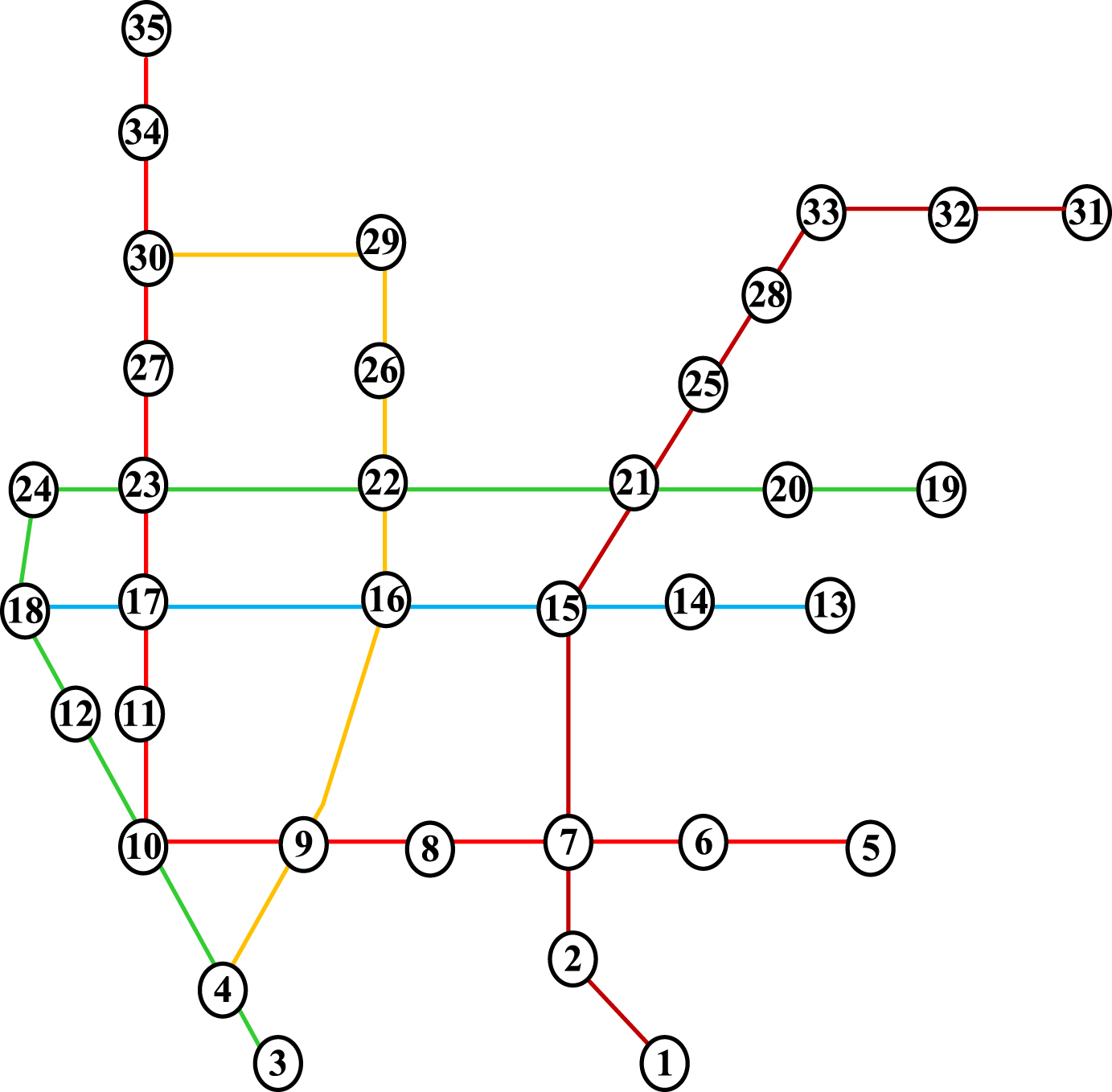
Locations of bike stations.

A-bike Company charges NT$20 per hour for the first 4 hours and NT$20 per hour (a half period rental) when the rental and return stations are the same. For each 30-minute block, the company charges NT$10 for the first 4 hours, NT$20 for the next 4 hours, and NT$40 for more than 8 hours. We divide a day into T = 12 equal time periods, each having two hours. Table 1 shows the number of bicycle docking piles for the 35 stations.

Table 1

Number of docking poles

i	D _i	i	D _i	i	D _i	i	D _i	i	D _i	i	D _i	i	D _i
1	66	6	34	11	44	16	42	21	52	26	31	31	36
2	38	7	57	12	54	17	63	22	56	27	39	32	56
3	38	8	72	13	47	18	58	23	28	28	50	33	39
4	49	9	46	14	16	19	26	24	61	29	70	34	52
5	51	10	59	15	53	20	50	25	48	30	49	35	52

The values of the required parameters were estimated as follows. The numbers of initial bicycles at the start of period 1, v_1i, were set at the entire value of 0.8D_i (Table 2).

Table 2

Number of initial bikes

i	v _1i	i	v _1i	i	v _1i	i	v _1i	i	v _1i	i	v _1i	i	v _1i
1	52	6	27	11	35	16	33	21	41	26	24	31	28
2	30	7	45	12	43	17	50	22	44	27	31	32	44
3	30	8	57	13	37	18	46	23	22	28	40	33	31
4	39	9	36	14	12	19	20	24	48	29	56	34	41
5	40	10	47	15	42	20	40	25	38	30	39	35	41

The minimum rental prices were set at NT$1 for all rental types. The demand markets for the company are assumed to follow a price dependent linear function d_tijk (p_tijk). The values of a_tijk were set at a_tijk = α_tβ_ijkD_i, in which parameters α_t are the time-variant scales and parameters β_ijk are the location and rental length-variant scales. The value of α_t is set at 0.1 for t = 1, 2, 3 and 12; 0.8 for t = 4, 9 and 10; 0.7 for t = 5; 0.6 for 6 ≤ t ≤ 8; and 0.4 for t = 11. The value of β_ijk was randomly generated over [0.004, 0.08] for k = 1, [0.004, 0.06] for k = 2, and [0.004, 0.035] for k = 3 under $\sum_{j = 1}^{M} \sum_{k = 1}^{K} β_{ijk} = 1$ . The values of the price elastics b_tijk were randomly generated over $[a_{tijk} / p_{tijk}^{o}, 1.8 a_{tijk} / p_{tijk}^{o}]$ , where $p_{tijk}^{o}$ is the original rental price. We use symbols $a_{tijk}^{o}$ , $b_{tijk}^{o}$ , and $v_{1 i}^{o}$ to represent the values of a_tijk, b_tijk, and v_1i, respectively, as set and referred as basic values.

4.2. Testing Problems

Five types of problems were designed, and seven cases were generated for each problem type. The number of bicycle stations is set to five for Problem type 1 and 35 for Problem types 3-5. For Problem type 2, the number of bicycle stations is incremental from 5 to 35. The values of all parameters in all cases of all the problem types are the same as that set in the previous section, except for the following changes.

In Problem types 1 and 3, we change the number of initial bicycle incrementally from 0.85 $v_{1 i}^{o}$ to 1.15 $v_{1 i}^{o}$ with 0.05 equal-percentage increment. In Problem type 4, we change the value of demand coefficient incrementally from 0.85 $a_{tijk}^{o}$ to 1.15 $a_{tijk}^{o}$ . In Problem type 5, we change the value of demand coefficient b_tijk incrementally from 0.85 $b_{tijk}^{o}$ to 1.15 $b_{tijk}^{o}$ .

4.3. Computational results

Problem types 1-2 were used to evaluate the performance of the proposed solution procedure. To confirm the solution, we use the Lingo global solver to identify the global maximum for all instances. We use HS to stand for the proposed heuristic approach. The computational results confirm the following:

The Lingo global solver can produce feasible solutions within 4h CPU time for problem instances, in which the number of stations is not larger than 15. Among these results, the Lingo global solver could only confirm global optimums for all cases in Problem type 1.

For Problem type 1, Columns 4 and 7 of Table 3 show that the HS produces nearly the same solutions as those of the Lingo global solver. These solutions indicate that the HS and the Lingo global solver can produce optimal solutions for small size problems. In addition, Columns 6 and 10 reveal that the performance of the HS is better than that of the Lingo global solver in terms of computational times.

For Problem type 2, Columns 4 and 7 of Table 4 show that the solution gaps between the HS and the Lingo global solver are extremely close for the first three cases. These results corroborate that the HS can produce solutions in less computational time similar to those generated by the Lingo global solver in 4-hour CPU time limit for a middle-size problem.

From testing cases 4-6 of Problem type 2 and all testing cases in Problem types 3-5, we affirm that the Lingo global solver can no longer produce feasible solutions within 4-hour CPU time limit. However, the HS can still solve the problem within a reasonable CPU time (see Tables 4-7). Therefore, the proposed HS method can be applied to solve large-scale problems, which cannot be solved by the Lingo global solver within reasonable time limits.

Table 3
Computational results for Problem type 1

Lingo HGA

No. k S Rev SD Rev SD CPU RS ST

1 0.85 161 9318 331 9322 331 2 57.9 2.06

2 0.90 171 9323 332 9327 332 2 54.5 1.94

3 0.95 180 9328 334 9337 334 2 51.9 1.85

4 1.00 191 9327 334 9337 334 2 48.9 1.75

5 1.05 198 9324 333 9326 334 2 47.1 1.69

6 1.10 209 9314 334 9319 333 2 44.6 1.59

7 1.15 217 9303 332 9307 332 2 42.9 1.53

			Lingo	HGA
1	0.85	161	9318	331	9322	331	2	57.9	2.06
2	0.90	171	9323	332	9327	332	2	54.5	1.94
3	0.95	180	9328	334	9337	334	2	51.9	1.85
4	1.00	191	9327	334	9337	334	2	48.9	1.75
5	1.05	198	9324	333	9326	334	2	47.1	1.69
6	1.10	209	9314	334	9319	333	2	44.6	1.59
7	1.15	217	9303	332	9307	332	2	42.9	1.53

$v_{1 i} = {kv}_{1 i}^{o}$ , SD = number of bikes rented out.

Table 4

Computational results for Problem type 2

			Lingo		HGA
No.	M	S	Rev	SD	Rev	SD	CPU	RS	ST
1	5	191	9327	331	9337	334	2	48.9	1.75
2	10	403	29996	332	30001	1034	192	74.4	2.57
3	15	572	57116	334	57105	1902	843	99.8	3.33
4	20	761	N/A		93425	3041	1265	122.8	4.00
5	25	954	N/A		138744	4445	2087	145.4	4.66
6	30	1144	N/A		193243	6052	3031	168.9	5.29
7	35	1329	N/A		210855	8373	4400	158.7	6.30

Table 5

Computational results for Problem type 3

No.	v _1i	S	Rev	SD	RS	ST
1	0.85 $v_{1 i}^{o}$	1114	200435	6686	224.3	6.00
2	0.90 $v_{1 i}^{o}$	1181	253427	7016	214.6	5.94
3	0.95 $v_{1 i}^{o}$	1246	256099	7319	205.5	5.87
4	1.00 $v_{1 i}^{o}$	1329	258520	7670	194.5	5.77
5	1.05 $v_{1 i}^{o}$	1381	259426	7857	187.9	5.69
6	1.00 $v_{1 i}^{o}$	1449	260314	8029	179.7	5.54
7	1.05 $v_{1 i}^{o}$	1513	260915	8138	172.4	5.38

Table 6

Computational results for Problem type 4

No.	a _tijk	Rev	SD	AR	RS	ST
1	0.85 $a_{tijk}^{o}$	182459	6874	26.54	137.3	5.17
2	0.90 $a_{tijk}^{o}$	209468	7249	28.89	157.6	5.45
3	0.95 $a_{tijk}^{o}$	227575	7451	30.54	171.2	5.61
4	1.00 $a_{tijk}^{o}$	258520	7670	33.70	194.5	5.77
5	1.05 $a_{tijk}^{o}$	275583	7747	35.57	207.4	5.83
6	1.00 $a_{tijk}^{o}$	293590	7906	37.14	220.9	5.95
7	1.05 $a_{tijk}^{o}$	325824	7959	40.94	245.2	5.99

Table 7

Computational results for Problem type 5

No.	b _tijk	S	Rev	SD	RS	ST
1	0.85 $b_{tijk}^{o}$	1329	390252	8107	293.6	5.76
2	0.90 $b_{tijk}^{o}$	1329	313841	8201	236.1	6.10
3	0.95 $b_{tijk}^{o}$	1329	295750	7670	222.5	6.17
4	1.00 $b_{tijk}^{o}$	1329	258520	7669	194.5	5.77
5	1.05 $b_{tijk}^{o}$	1329	257599	7665	193.8	5.77
6	1.00 $b_{tijk}^{o}$	1329	254029	7689	191.1	5.77
7	1.05 $b_{tijk}^{o}$	1329	249054	7959	187.4	5.79

4.4. Sensitivity Analyses

Sensitivity analyses were performed to investigate the impact of the initial located bicycles, v_1i, and demand coefficients a_tijk and b_tijk on the computational results. We use initials RS = PR/S and ST = SD/S to represent the average rental revenue per bicycle and the average leased frequency per bicycle, respectively, where SD is the total number of biked rented out.

Problem types 1 and 3 investigates the impact of allocated number of bicycles on the computational results. The effects of the number of initial bicycles on the computational results are displayed in Tables 3 for small-scale problems (Problem type 1) and in Table 5 for large-scale problems (Problem type 3). From Columns 9 and 10 of Table 3 and Columns 7-8 of Table 5, the values of RS and ST decrease as the number of allocated bicycles, v_1i, and total number of bicycles, S, increases. Columns 4 and 5 of Table 5 shows that the revenues and number of bike rented out (SD) increase as the number of initial bicycles increases. This phenomenon fits the general cognition that considerable capacities can produce substantial sales and revenues. However, the results of Problem type 1 verify that this phenomenon does not always hold. Column 4 of Table 3 shows that the revenues increase as the number of initial bicycles increases. However, when the value of v_1i reaches $0.95 v_{1 i}^{o}$ , the revenue begins to descend. The reason may be that the number of available docking poles decreases with the number of bicycles allocated. A demand is composed of a rental and a return service; thus, insufficient bicycle docking poles may result in lost sales. The phenomenon reflects that considerable capacities cannot guarantee the generation of substantial sales and revenues. The number of initial bicycles allocated currently is suitable for the network with five bicycle stations. We can also affirm that the marginal revenue decreases as the number of bicycles increases.

Problem type 2 investigates the impact of the number of bicycle stations on the computational results. As shown in Columns 4 and 10 of Table 4, the revenues and the values of ST have increasing tendencies when the number of bicycle stations increases. The reason may be that bicycle stations in a big bicycle network can cover more demands compared with those having few bicycle stations.

Problem type 4 investigates the impact of parameter a_tijk on computational results. In this case, the total number of bikes is 1329. Columns 4, 7, and 8 of Table 6 show that the revenues, RS, and ST increase as the values of a_tijk increase. In addition, we affirm that the average rental price (AR) also increases with the values of a_tijk.

Problem type 5 investigates the impact of price elastic on the computational results. Columns 4, 7, and 8 of Table 7 show that the revenues and RS decrease with the price elastic. The reason may possibly be the negative impact of price elasticity on demand.

5. Conclusion and Future Work

This study develops a constrained mathematical model to solve a rental pricing problem for bicycle rental companies. Our results confirm that the solutions to the KKT system of equations are the optimal sale prices. We develop a heuristic algorithm, which is based on mathematical programming, and an evolutionary algorithm to efficiently solve the problem. Computational results validate that the proposed approach can find optimal solutions for small-scale problems and can produce solutions that the Lingo global solver cannot produce feasible solutions within a reasonable CPU time. Sensitivity analyses were also conducted to investigate the effects of various system parameters.

In this study, we propose a demand management approach to balance the bicycle levels among the bicycle networks. The supply management approach based on the bicycle transfer of rental companies is also an efficient approach to balance the bicycle levels. Simultaneously adapting the two approaches to balance bicycle systems is also possible. To analyze this case, we should reformulate the mathematical model and develop new methods to solve the problem. This study is complex, hence will be further studied.

References

G.J.

Beaujon and

M.A.

Turnquist , A model for fleet sizing and allocation, Transportation Science 25 (1991), 14–45.

Benchimol ,

Chappert ,

A.D.L.

Taille ,

Laroche ,

Meunier and

Robinet , Balancing the stations of a self-service bike hire system, RAIRO Operations Research 45 (2011), 37–61.

Benigno ,

Guerriero and

Miglionico , A revenue management approach to address a truck rental problem, Journal of the Operational Research Society 63 (2012), 1421–1433.

Chemla ,

Meunier and

Wolfler Calvo , Bike sharing systems: Solving the static rebalancing problem, Discrete Optimization 10 (2013), 120–146.

W.C.

Chiang ,

J.C.H.

Chen and

Xu , An overview of research on revenue management: Current issues and future research, International Journal of Revenue Management 1 (2007), 97–128.

E.G.

Erdoğan ,

Laporte and

R.W.

Calvo , The static bicycle relocation problem with demand intervals, European Journal of Operational Research 238 (2014), 451–457.

Erdogan ,

Battarra and

Wolfler Calvo , An exact algorithm for the static rebalancing problem arising in bicycle sharing systems, European Journal of Operational Research 245 (2015), 667–679.

A.T.

Ernst ,

Horn ,

Kilby and

Krishnamoorthy , Dynamic scheduling of recreational rental vehicles with revenue management extensions, Journal of the Operational Research Society 61 (2010), 1133–1143.

A.T.

Ernst ,

E.O.

Gavriliouk and

Marquez , An efficient Lagrangean heuristic for rental vehicle scheduling, Computers & Operations Research 38 (2011), 216–226.

10.

Fink and

Reiners , Modeling and solving the shortterm car rental logistics problem, Transportation Research E 42 (2006), 272–292.

11.

D.K.

George and

C.H.

Xia , Fleet-sizing and service availability for a vehicle rental system via closed queuing networks, European Journal of Operational Research 211 (2011), 198–207.

12.

Guerriero and

Olivito , Revenue models and policies for the car rental industry, Journal of Mathematical Modelling and Algorithms in Operations Research 13 (2014), 247–282.

13.

S.C.

Ho and

W.Y.

Szeto , Solving a static repositioning problem in bike-sharing systems using iterated tabu search, Transportation Research E 69 (2014), 180–198.

14.

Kochel ,

Kunze and

Nielander , Optimal control of a distributed service system with moving resources: Application to the fleet sizing and allocation problem, International Journal of Production Economics 81/82 (2003), 443–459.

15.

B.B.

Oliveira ,

M.A.

Carravilla ,

J.F.

Oliveira and

M.B.

Toledo , A relax-and-fix-based algorithm for the vehicle-reservation assignment problem in a car rental company, European Journal of Operational Research 237 (2014), 729–737.

16.

Ogilvie and

Goodman , Inequalities in usage of a public bicycle sharing scheme: Socio-demographic predictors of uptake and usage of the London (UK) cycle hire scheme, American Journal of Preventive Medicine 55 (2012), 40–45.

17.

Papazek ,

Raidl ,

Rainer-Harbach and

Hu , A PILOT/ VND/GRASP hybrid for the static balancing of public bicycle sharing systems, In: Computer Aided Systems Theory-EUROCAST, Springer, 2013, pp. 372–379.

18.

Papier and

U.W.

Thonemann , Capacity rationing in rental systems with two customer classes and batch arrivals, Omega 39 (2011), 73–85.

19.

Rainer-Harbach ,

Papazek ,

G.R.

Raidl ,

Hu and

Kloimiillner , PILOT, GRASP, and VNS approaches for the static balancing of bicycle sharing systems, Journal of Global Optimization 63 (2014), 597–629.

20.

Raviv ,

Tzur and

Forma , Static repositioning in a bikesharing system: Models and solution approaches, EURO Journal on Transportation and Logistics 2 (2013), 187–229.

21.

Raviv and

Kolka , Optimal inventory management of a bikesharing station, IIE Transactions 45 (2013), 1077–1093.

22.

S.V.

Savin ,

M.A.

Cohen ,

Gans and

Katalan , Capacity management in rental businesses with two customer bases, Operations Research 53 (2005), 617–631.

23.

H.R.

Sayarshad and

Ghoseiri , A simulated annealing approach for the multi-periodic rail-car fleet sizing problem, Computers & Operations Research 36 (2009), 1789–1799.

24.

H.R.

Sayarshad and

Tavakkoli-Moghaddam , Solving a multi periodic stochastic model of the rail-car fleet sizing by two-stage optimization formulation, Applied Mathematical Modelling 34 (2010), 1164–1174.

25.

H.R.

Sayarshad ,

Tavassoli and

Zhao , A multi-periodic optimization formulation for bike planning and bike utilization, Applied Mathematical Modelling 36 (2012), 4944–4951.

26.

D.P.

Song and

Carter , Optimal empty vehicle redistribution for hub-and-spoke transportation systems, Naval Research Logistics 55 (2008), 156–171.

27.

W.Y.

Szeto ,

Liu and

S.C.

Ho , Chemical reaction optimization for solving a static bike repositioning problem, Transportation Research Part D 47 (2016), 104–135.

28.

K.T.

Talluri and

G.J.

van Ryzin , The Theory and Practice of Revenue Management, Springer, Boston, 2004.

29.

Yaghini and

Khandaghabadi , A hybrid metaheuristic algorithm for dynamic rail car feet sizing problem, Applied Mathematical Modelling 37 (2013), 4127–4138.

30.

P.S.

You ,

P.J.

Lee and

Y.C.

Hsieh , An artificial intelligent approach to the bicycle repositioning problems, Engineering Computations 34 (2017), 145–163.