Pair wise training for stacked convolutional autoencoders using small scale images

Abstract

Deep neural networks have dramatically gained immense potential in almost every field like computer vision, natural language processing, biomedical informatics etc. Among these networks, autoencoders are popular in performing dimensionality reduction task, while learning a representation for an unlabeled dataset. A usual way of dealing with such networks is to pre-train them in a layer-wise fashion, and consequently fine-tune the whole stack in a supervised manner. In this paper, a pair-wise training strategy is proposed to determine optimum model parameters by reducing training time as well as the complexity of training a convolutional autoencoder without compromising its accuracy. The proposed approach works in a fully unsupervised manner and has been tested on datasets like MNIST, CIFAR10, and CIFAR100 and it shows that the training time has improved by an average of 25% on these three datasets.

Keywords

Deep learning convolutional autoencoder pair-wise training

1. Introduction

Deep learning is about artificial neural networks which receive input and perform progressively complex calculations on them to get an output. A neural network which is trained on a particular problem should be able to solve a similar problem as well. As an input pattern gets more complex, neural networks with a small number of layers and very fewer nodes become insufficient to handle them. It is seen that the number of nodes required at each layer grows exponentially with the number of possible patterns in data [10]. This eventually makes training too expensive and accuracy of the whole network starts to suffer. So, for an intricate pattern like face of a human, basic classification algorithms or shallow neural networks are inadequate. Deep learning algorithms are able to break down these complicated patterns into a series of simple patterns. As more complex or deeper networks are needed to learn complex patterns, training these networks from scratch is still an issue.

In 2006, Hinton et al. [8] verified that unsupervised greedy layer wise training approach typically helps in optimizing deep belief networks. Bengio et al. [2] later on studied this fact and confirmed that it is possible to do a better generalization using this training strategy. This was a breakthrough in the domain of neural networks and deep neural networks started to conquer the world. An upsurge of convolutional neural networks (CNN) has made significant improvements in the field of object recognition also. They have been widely used for classification task by training them in a supervised manner [1, 23]. But as it requires a large amount of labeled training data [11], the learning becomes deliberate and time consuming. Though this was overcome by fine tuning a pre-trained network with the available small dataset, it is not applicable in every situation. For example, if the dataset is very indifferent from pre-trained network’s data. In such cases, the entire network should be trained from scratch. So in 2015, Rueda-Plata et al. [22] proposed a greedy layer wise method to train deep convolutional networks on small datasets in supervised manner without using any pre-trained models.

In real life situations like medical imaging, it is very tedious, time consuming, and expensive to get such huge datasets to be labeled by two or more experts. In such cases, an unsupervised approach is practically more dependable than supervised techniques. Autoencoder is one such popular neural network that learns representation for an unlabeled dataset. Apart from other neural nets, autoencoders are traditionally used to perform dimensionality reduction and these learned weights are then used to initialize another neural network. The layers function as restricted Boltzmann machines (RBM) which makes the building blocks of deep-belief networks (DBN). Interestingly, an autoencoder tries to reconstruct the input by learning hierarchical features of data through a stack of encoding and decoding layers in an unsupervised manner.

The encoder and decoder, which can be defined as transitions φ and ψ, functions as two parts of the autoencoder such that,

$φ, ψ = \underset{φ, ψ}{argmin} ∥ X - (ψ \circ φ) X ∥^{2}$ (1)

where φ (X) is the coded representation of the input X and ψ (φ (X)) is the output from decoder. In Equation (1), as ψ tries to reconstruct the output from the encoder φ, the objective of autoencoder is to minimize the loss between actual input and the reconstructed output. The gradient of the error between original input and the output obtained is fed back to the network to update the weights.

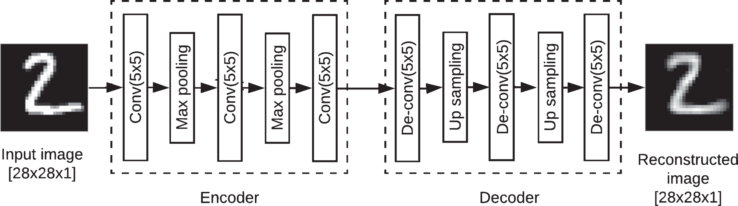
The major difference between a standard autoencoder (shown in Fig. 1) and a convolutional autoencoder is that the latter has convolutional layers in the encoding section and deconvolution layers in the decoding section. The encoding layers compress the input image into a different feature space and decoding layers try to reconstruct the image from the compressed feature vector. The network is made to learn till it is able to reproduce the inputs that it has not seen before. Usually, it is difficult to train a stacked convolutional autoencoder from scratch [16]. The situation is even worse with high resolution images.

Fig. 1

Schematic structure of an autoencoder.

In this paper, a pair-wise approach to train stacked convolutional autoencoder (SCAE) is proposed, which reduces the training time by 25% when compared to the usual end to end training procedure. Rest of this paper is organized as follows. In section 1, most beneficial related works that have helped us throughout this research work is presented. Then a detailed discussion of the proposed work is presented in section 1. In section 1, details of the experimental works that are conducted during studies, the dataset description, and the system architecture are included. The results and findings are summarized in section 1.

2. Related works

A standard stacked autoencoder, which is formed by stacking multiple autoencoders is learned by pre-training each layer before its successor using backpropogation algorithm. After the successful introduction of these networks, a wide variety of autoencoders including denoising autoencoders were proposed. In 2011, Masci et al. [17] introduced the concepts of convolutional autoencoders for the first time due to the fact that autoencoders and denoising auto encoders, both ignore the two dimensional structure of image data. They suggested that convolutional autoencoders can be used as a weight initializer for supervised methods like deep convolutional neural networks. The authors tested the model with several datasets and confirm that the model learns hierarchical features from the input images and thus act as a feature extractor.

Mandar Kulkarni and Shirish Karande [13] proposed a kernel similarity based optimization approach for layer-wise training of a deep neural network for supervised classification task. In each layer, a kernel is defined and is optimized so that it comes up with the best kernel where data points that belong to the same class have kernel value equal to 1 while data points from different classes have kernel value equal to 0. Results indicate that the proposed approach is comparable with deep neural networks.

Alireza Makhzani and Brendan Frey [15] suggested a winner-take-all method for learning hierarchical sparse representations in convolutional autoencoders in an unsupervised fashion. Turchenko et al. [25] created five different models of autoencoders and most of them had achieved very good performance in dimensionality reduction as well as unsupervised clustering tasks. Mao et al. [16] developed a fully convolutional autoencoder for image restoration and it consisted of many convolution and deconvolution layers symmetrically arranged in a chain fashion. The model did not include any pooling or unpooling layers, since the aim was to eliminate low level corruption. They had used skip connection to update filters in the initial layers of the model efficiently. They stated that the network achieved better performance than state-of-the-art methods on different techniques such as image denoising, image super-resolution etc.

Valpola et al. [21] proposed a network with ladder structure and Rasmus et al. [20] extended this work by combining it with supervised technique and they showed the enhanced classification accuracy on both MNIST and CIFAR-10 datasets. Recently, Du et al. [5] interestingly investigated the quality of features learned by deep architectures obtained by stacking autoencoders. The model was constructed by stacking denoising autoencoders whose parameter values were optimized through patch-wise training. They proposed a layer wise whitening technique which proved to be an efficient method for classification task.

3. Proposed system

Traditionally, convolutional autoencoders are used for general purpose feature extraction or dimensionality reduction as well as to initialize network weights. These networks are generally learned in an end to end fashion by minimizing the difference between input and the reconstructed output. But during the training, it uses backpropagation algorithm to compute the gradient of the error function which can make the networks too long to train especially when the networks are deep enough. Hence this work proposes a pair-wise training approach for the reconstruction of images.

This concept is much like deep belief networks (DBN) [2, 12] that are made of stacking restricted boltzmann machines (RBM) [8, 18]. In DBN, each RBM is trained completely and the output obtained is passed on to next RBM and so on. Unlike usual end to end training procedure using backpropogation, the proposed system has several individual reconstruction phases that learn two layers of the model at a time. In each reconstruction phase, the input image is convolved to a feature space and reconstructed back by deconvolving it. In between the convolution and deconvolution layers, pooling and unpooling layers can be added.

The stacked convolutional autoencoder has an architecture as shown in Fig. 2. Since the same input image is to be reconstructed, the input and output layers are chosen to have the same dimensions. For better performance, the weight parameters of the network were initialized using Xavier initialization method [7] instead of random initialization. The normalized initialization is shown in Equation (2).

Fig. 2

Architecture of model on which proposed training concept is implemented.

$W \sim U [- \frac{\sqrt{6}}{\sqrt{n_{j} + n_{j + 1}}}, \frac{\sqrt{6}}{\sqrt{n_{j} + n_{j + 1}}}]$ (2)

where n_j is the size of layer j. According to Glorot et al. [7], this effectively helps in reducing training time required for the network.Input layer receives the 28x28 resolution image that is convolved with 6 filters with zero padding. Size of the filters is set to be 5x5 so that it captures even minute features from the input. The max pooling layer with a sampling rate 2, is appended and again convolved with 16 filters of size 5x5. This is continued in the encoding section and finally a feature set with dimension of 1x120 is obtained. Here the max pooling layer is included as it is a smart way to implement sparse code needed to deal with the over complete representations of convolutional architectures.

In decoding section, corresponding deconvolution and up-sampling are done carefully and symmetrically to regain original input image. The whole model with a total parameters 1,01,265 is trained for 50 epochs. In first step, there are only 307 parameters to train, in second step, 4,822 parameters and final step has 96,136 parameters. This demonstrates the easiness in training as the parameters are learned in individual stages rather than learning it as a whole. The model summary for MNIST is as shown in Table 1. Number of parameters to be trained slightly vary with different datasets.

Table 1

Model summary for MNIST

Layer	Input	Filter size	# filters	Padding	Output	# parameters
Conv1	28x28x1	5x5	6	2	28x28x6	156
Pool1	28x28x6	2x2		–	14x14x6	0
Conv2	14x14x6	5x5	16	–	10x10x16	2416
Pool2	10x10x16	2x2		–	5x5x16	0
Conv3	5x5x16	5x5	120	–	1x1x120	48120
Conv3_Transpose	1x1x120	5x5	16	–	5x5x16	48016
Upsampling_2	5x5x16	2x2		–	10x10x16	0
Conv2_Transpose	10x10x16	5x5	6	–	14x14x6	2406
Upsampling_1	14x14x6	2x2		–	28x28x6	0
Conv1_Transpose	28x28x6	5x5	1	2	28x28x1	151

At first, the network is initialized with just two layers namely a convolution layer and a deconvolution layer. The layer weights are initialized using Xavier method [7] and trained using categorical cross entropy loss function. ADADELTA [27] is used as the optimizing parameter for learning rate as this method requires no manual tuning of a learning rate and found to be vigorous to noisy gradient information. When the two layers are finished training, they are frozen out [3] and the next pair of convolution-deconvolution layers are added and trained similarly.

When a layer is frozen, all its parameters are not updated during training of the entire model (both in forward and backward pass). This depicts the simplicity of the model as it is training only a single pair of layers at a time. Fig. 3(a), (b) and (c) shows different stages in the training phase where the gray color indicates the current training pair. The whole procedure is formally stated in Algorithm 1.

Fig. 3

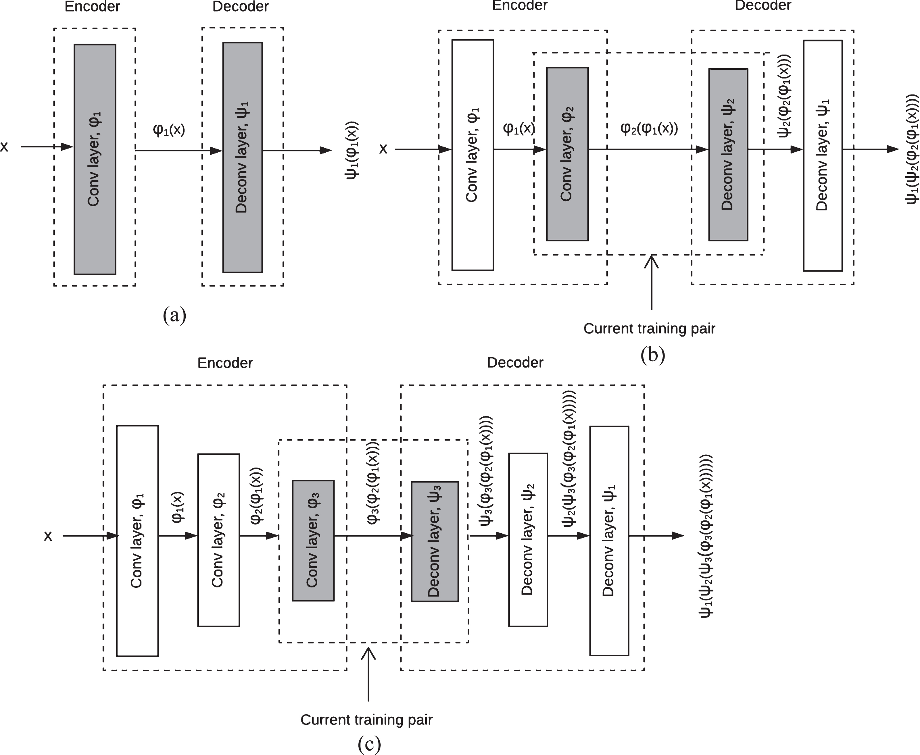
Training stages. (a) First pair of layers are trained, (b) second pair is inserted and trained while first layer is frozen and (c) third pair is inserted and trained while first and second pair are frozen. Gray color indicates the current training pair.

Let φ_i and ψ_i be the i^th pair of encoder and decoder to be trained. Then from Equation (1) the objective function for the first pair can be redefined as $φ, ψ = \underset{φ, ψ}{argmin} ∥ X_{1} - (ψ_{1} \circ φ_{1}) X_{1} ∥^{2}$ (3) and for the second pair as $φ, ψ = \underset{φ, ψ}{argmin} ∥ X_{2} - (ψ_{2} \circ φ_{2}) X_{2} ∥^{2}$ (4) Similarly for n^th pair, $φ, ψ = \underset{φ, ψ}{argmin} ∥ X_{n} - (ψ_{n} \circ φ_{n}) X_{n} ∥^{2}$ (5) where as the end to end training computes $φ, ψ = \underset{φ, ψ}{argmin} ∥ X - (ψ_{1} \circ ψ_{2} \circ . . . \circ ψ_{n} \circ φ_{n} \circ φ_{n - 1} . . . \circ φ_{1}) X ∥^{2}$ (6) In short, we try to reduce the complexity of training by considering individual pairs in the whole network rather than training it at a single stretch.

4. Experiments and results

4.1 Dataset

Three most familiar small scale datasets were used to test the training efficiency of layer-wise training of stacked convolutional autoencoders as well as end to end training time of the same. The main properties of these datasets are described in Table 2.

Table 2
Description of Datasets

Dataset # train images # test images Image resolution Type

MNIST 60000 10000 28x28 Grayscale

CIFAR10 50000 10000 32x32 Color

CIFAR100 50000 10000 32x32 Color

Dataset	# train images	# test images	Image resolution	Type
MNIST	60000	10000	28x28	Grayscale
CIFAR10	50000	10000	32x32	Color
CIFAR100	50000	10000	32x32	Color

Algorithm 1 Pair wise training of SCAE
Initialize the network, N with a pair of encoder, φ and
decoder, ψ.
n ← total _ number _ of _ pairs
i ← 1
for each pair, ido
for each feature map, x_ido
compute φ (x_i) and ψ (φ (x_i))
measure the deviation of ψ (φ (x_i)) from the
input feature map, x_i
update the weights of i^th pair
end for
if i + 1 ≤ nthen
freeze the current pair of layers
add (i + 1) ^th pair in between the i^th pair
end if
end for

MNIST [28] contains handwritten digits of 60000 training and 10000 testing images each one having resolution 28x28. It contains real-world grayscale images that need minimal efforts on preprocessing and formatting. CIFAR10 dataset [29] consists of 60000 color images with a resolution of 32x32. It has only 10 categories whereas CIFAR100 dataset [29] has 100 categories of images. An imperative advantage of small scale images is that they require very less amount of memory space for storage as well as manipulation of datasets whose magnitude is greater than those usually used in computer vision applications. Mostly low resolution images are preferable since they retain vital information regarding the visual world by preserving the semantic content.

4.2 Methodology

The model was initially trained with MNIST in an end to end fashion and was seen to converge in 50 epochs. It was then validated with test data and was giving a validation accuracy of 81%. When tested with a sample of images, the network was also able to reconstruct input images with some loss of information.

Later on, proposed approach was implemented in the same model and training was done in pair-wise manner with MNIST dataset. First pair of layers was trained for about 10 epochs and it was giving almost 79% of accuracy. That means it was able to do the reconstruction of the image with just two layers. But this was not enough as a more compressed form of data representation were needed. A model will be efficient only if it can perform reconstruction with minimum possible relevant feature set. Table 3 shows the tabulated form of experimental results obtained during training. The difference in training time is clearly visible as the number of parameters increase. All experimental works were done using Keras library [30] with Tensorflow [31] as backend.

Table 3
Final results obtained with MNIST, CIFAR10 and CIFAR100 on the two approaches

Architecture Epochs Time (min) #parameters

MNIST (end-to-end) 50 43 1,01,265

MNIST (pair-wise) 50 33 1,01,265

CIFAR10 (end-to-end) 50 81 1,01,867

CIFAR10 (pair-wise) 50 62 1,01,867

CIFAR100 (end-to-end) 50 82 1,01,867

CIFAR100 (pair-wise) 50 60 1,01,867

Architecture	Epochs	Time (min)	#parameters
MNIST (end-to-end)	50	43	1,01,265
MNIST (pair-wise)	50	33	1,01,265
CIFAR10 (end-to-end)	50	81	1,01,867
CIFAR10 (pair-wise)	50	62	1,01,867
CIFAR100 (end-to-end)	50	82	1,01,867
CIFAR100 (pair-wise)	50	60	1,01,867

As expected, there were no visible differences between two strategies other than the training time. In fact, the features learned and accuracy remained untouched. Fig. 4 depicts the input images (first row) and corresponding reconstructed images (second row) during pair wise training. And as shown in figure, the model was nearly able to regain the original structure of the digits in the test images as some information was lost during the decoding process. Though the model is not 100% successful in reconstructing the input, it tries to develop an approximate or estimated output from the given image using the learned features.

Fig. 4

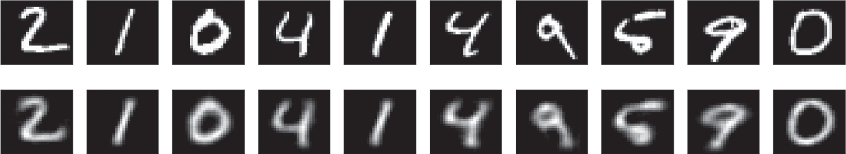
Test input images (first row) and reconstructed output images (second row) during pair wise training of SCAE using MNIST dataset.

When the first pair was done with the training, they were frozen so that the next level of learning occurs only in second pair of layers. Therefore, the second pair starts learning only when the first pair has fully learned the images. The second pair also converges within a few epochs.The final pair takes a little more time to converge as it has more number of parameters than the previous ones. The third pair creates a feature vector with dimension 1x120 which is the encoded form of the initial 28x28 image. If needed, this feature vector can be further used as an input for supervised models that can perform classification. Fig. 5(a) depicts the overall loss obtained during the existing end to end training whereas Fig. 5(b), (c) and (d) shows the loss for pair I, pair II and pair III respectively at each epoch. From the figure, we observed that the losses for a network trained by both end to end and pair wise techniques are almost same (see Fig. 5(a) and 5(d)) and hence the accuracy.

A similar work done by Alireza Makhzani and Brendan [15] proposes a winner-take-all method to learn shift-invariant sparse features in convolutional autoencoders. They have used a hierarchical approach in order to train the network whose building blocks are individual convolutional winner-take-all autoencoders (CONV-WTA). Initially, all the images are passed on to a single CONV-WTA and the shift-invariant features are learned at a stretch. Then the images are again passed on to the network to extract the features. These feature maps are given as input to the next CONV-WTA for further feature learning and this can be repeated to obtain the entire stack of representations. Thus the images are passing through each autoencoder twice; one for feature learning and another for feature extraction. The motivation behind building such a hierarchical structure was to efficiently train networks with large datasets.

The technique which was proposed is distinct from the stated method in following regards. Pair-wise approach intuitively eliminates the burden of the network with a single pass. As the images are passed on to the frozen layers, features are extracted automatically and hence there is no need for an extra pass especially for this purpose. The network also achieves the same accuracy as that of the described method when compared with MNIST and CIFAR datasets and it is also favorable for training huge image datasets.

Fig. 5

Results of quantitative experiments on MNIST. (a) Loss obtained during end to end training; (b), (c) and (d) are the losses during pair wise training of pair I, pair II and pair III respectively.

To summarize, two models were created; one for MNIST and another for CIFAR10 and CIFAR100 (as they have same input parameters). These models were compared on the basis of training time given by the two approaches and the results are shown in Fig. 6. Results obtained shows that the training time for MNIST was decreased by 23%, and for CIFAR10 and CIFAR100, it decreased by 27% resulting in an overall improvement of training time by an average of 25% by using the proposed method.

Fig. 6

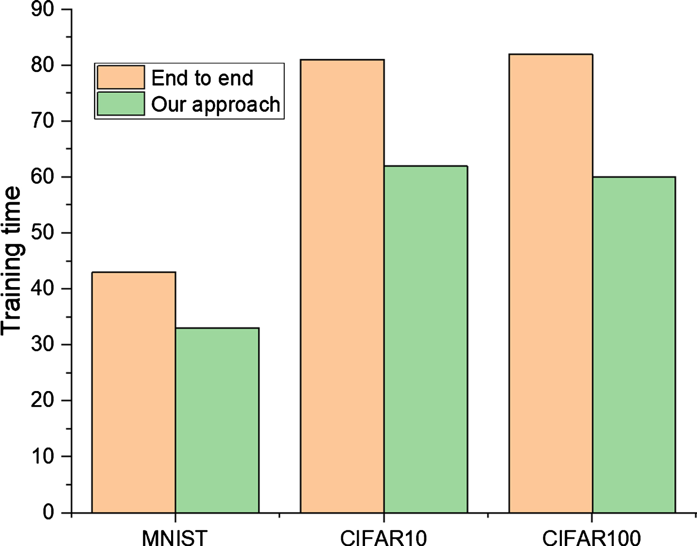
A comparison on end to end and pair-wise training on MNIST, CIFAR10 and CIFAR100.

5. Conclusions

The work intends to improve the training efficiency of stacked convolutional autoencoders without compromising accuracy. An average reduction of 25% of training time was achieved through proposed pair-wise approach and appropriate initialization of parameters. Though the two network architectures employed actually differ only by about 600 parameters as shown in Table 3, time needed for training has reduced significantly by using the proposed method. From the results obtained, it is obvious that this approach is beneficial for deeper networks with a large amount of training parameters and insufficient labeled data as there is a visible difference in training time of the networks with an increase in parameters.

Footnotes

Acknowledgement

This research was made possible by grants and support from the Council of Scientific & Industrial Research and Amrita Vishwa Vidyapeetham. We would also like to thank Mr. M R Kaimal and Mr. Gopakumar G, Amrita Vishwa Vidyapeetham for their valuable comments.

References

Anil ,

Manjusha ,

S.S.

Kumar and

Soman , Convolutional neural networks for the recognition of Malayalam characters, Proceedings of the 3rd International Conference on Frontiers of Intelligent Computing: Theory and Applications (FICTA), Springer, 2015, pp. 493–500.

Bengio ,

Lamblin ,

Popovici and

Larochelle , Greedy layerwise training of deep networks, Advances in Neural Information Processing Systems (2007), 153–160.

Brock ,

Lim ,

Ritchie and

Weston , Freezeout: Accelerate training by progressively freezing layers, Paper presented at 10th NIPS Workshop on Optimization for Machine Learning, United States, 2017.

Chen ,

Shi ,

Zhang ,

Wu and

Guizani , Deep features learning for medical image analysis with convolu-tional autoencoder neural network, IEEE Transactions on Big Data 1 (2017).

Du ,

Xiong ,

Wu ,

Zhang ,

Zhang and

Tao , Stacked convolutional denoising auto-encoders for feature representation, IEEE Transactions on Cybernetics 47(4) (2017), 1017–1027.

Erhan ,

Manzagol ,

Bengio ,

Bengio and

Vincent , The difficulty of training deep architectures and the effect of unsupervised pre-training, Proceedings of the 12th International Conference on Artificial Intelligence and Statistics, 2009, pp. 153–160.

Glorot and

Bengio , Understanding the difficulty of training deep feedforward neural networks, Proceedings of the 13th International Conference on Artificial Intelligence and Statistics, 2010, pp. 249–256.

G.E.

Hinton and

R.R.

Salakhutdinov , Reducing the dimensionality of data with neural networks, Science 313(5786) (2006), 504–507.

G.E.

Hinton ,

Osindero and

Y.W.

Teh , A fast learning algorithm for deep belief nets, Neural computation 18(7) (2006), 1527–1554.

10.

Hwang and

Chen , Big-Data Analytics for Cloud, IoT and Cognitive Computing, JohnWiley & Sons, New York, USA, 2017.

11.

M.A.

Islam ,

Bruce and

Wang , Dense image labeling using deep convolutional neural networks, 13th IEEE Conference on Computer and Robot Vision (CRV), 2016, pp. 16–23.

12.

Jagadeesh ,

Anand Kumar and

K.P.

Soman , Deep belief network based part-of-speech tagger for telugu language, Proceedings of 2nd International Conference on Computer and Communication Technologies, Springer, New, Delhi, 2016, pp. 75–84.

13.

Kulkarni and

Karande , Layer-wise training of deep networks using kernel similarity, 2017, arXiv preprint arXiv: 1703.07115.

14.

Liu ,

Zhang and

Ma , Stacked auto-encoders for feature extraction with neural networks, International Conference on Bio-Inspired Computing-Theories and Applications, Springer, Singapore, 2016, pp. 377–384.

15.

Makhzani and

Frey , A winner-take-all method for training sparse convolutional autoencoders, Neural Information Processing Systems (NIPS) Deep Learning Workshop (2014).

16.

X.J.

Mao ,

Shen and

Y.B.

Yang , Image restoration using convolutional auto-encoders with symmetric skip connections, Advances in Neural Information Processing Systems(NIPS), 2016.

17.

Masci ,

Meier ,

Ciresan and

Schmidhuber , Stacked convolutional auto-encoders for hierarchical feature extraction, International Conference on Artificial Neural Networks and Machine Learning(ICANN), 2011, pp. 52–59.

18.

Midhun ,

S.R.

Nair ,

Prabhakar and

S.S.

Kumar , Deep model for classification of hyperspectral image using restricted boltzmann machine, Proceedings of the 2014 International Conference on Interdisciplinary Advances in Applied Computing, ACM, 2014, pp. 1–7.

19.

Mirza ,

Syed ,

Memon and

Malik , Ladder Networks: Learning under massive label deficit, International Journal of Advanced Computer Science and Applications 8(7) (2017), 502–507.

20.

Rasmus ,

Raiko and

Valpola , Denoising autoencoder with modulated lateral connections learns invariant representations of natural images, 2015, arXiv preprint arXiv: 1412.7210.

21.

Rasmus ,

Valpola ,

Honkala ,

Berglund and

Raiko , Semi-supervised learning with ladder networks, Advances in Neural Information Processing Systems (2015), 3546–3554.

22.

Rueda-Plata ,

Ramos-Pollan and

F.A.

Gonz'alez , Supervised greedy layer-wise training for deep convolutional networks with small datasets, Computational Collective Intelligence, Springer (2015), 275–284.

23.

K.S.

Sahla and

Senthil Kumar , Classroom teaching assessment based on student emotions, The International Symposium on Intelligent Systems Technologies and Applications, Springer, 2016, pp. 475–486.

24.

C.K.

Sonderby ,

Raiko ,

Maaloe ,

S.K.

Sonderby and

Winther , Ladder variational autoencoders, Advances in Neural Information Processing Systems (2016), 3738–3746.

25.

Turchenko ,

Chalmers and

Luczak , A deep convolutional auto-encoder with pooling-unpooling layers in caffe, 2017, arXiv preprint arXiv: 1701.04949.

26.

Vincent ,

Larochelle ,

Lajoie ,

Bengio and

Manzagol , Stacked denoising autoencoders: Learning useful representations in a deep network with a local denoising criterion, Journal of Machine Learning Research 11 (2010), 3371–3408.

27.

M.D. Zeiler, Adadelta: An adaptive learning rate method, Technical report, 2012.

28.

http://yann.lecun.com/exdb/mnist/

29.

https://www.cs.toronto.edu/kriz/cifar.html

30.

https://keras.io

31.

https://www.tensorflow.org