Meta-type fuzzy computations and fuzzy complexity

Abstract

We define a meta-type (MFTM) of Fuzzy Turing Machines (FTM) in which the transitions can take dynamic degrees corresponding with the input. The advantage of MFTM over other FTMs previously defined in the literature is that, by applying the dynamic degrees of transitions, it can resolve a deficiency in recognizing the fuzzy languages where their elements have arbitrary different non-crisp degrees. This results in recognizing a larger class of fuzzy languages than the other FTMs. Also, we establish a fuzzy theory of computational complexity and introduce two complexity classes FP and FNP for fuzzy polynomial time-bounded (deterministic and non-deterministic) computations. We propose fuzzy variants of three problems namely, finding a path (PATH) and a Hamiltonian path (HAMPATH) in a digraph and SAT problem. We show that the fuzzy variant of PATH is in FP while the ones of SAT and HAMPATH are in FNP. We introduce the class of FNP-complete problems and show that fuzzy variants of SAT, 3-SAT and HAMPATH are FNP-complete.

Keywords

Fuzzy Turing Machine Meta fuzzy Turing Machine fuzzy reducibility fuzzy complexity fuzzy SAT fuzzy HAMPATH

1 Introduction

Lotfi Zadeh defines the notion of fuzzy algorithms in [12], based on a fuzzification of Turing machines and Markov algorithms. This line is followed by some works like [4 , 9]. Then, the research in this subject is untouched for more than a decade and revisited only in [3]. Next, Wiedermann considers computability and complexity of fuzzy computation in [11]. He claims that fuzzy Turing machines (FTMs) have more computational power than the classical Turing machines and could accept non-recursively enumerable sets. In [1], Bedregal and Figueira show that Wiedermann’s statement is not completely correct and also show that there is no universal fuzzy Turing machine which can simulate every fuzzy Turing machine. Afterward, Li studies some variants of fuzzy Turing machines in [5]. He shows that there is no universal FTM that can simulate any FTM, but a universal FTM exists in some approximate sense. He also introduces the notion of fuzzy polynomial time complexity and gives a special fuzzy variant of classical satisfiability problem (SAT). In [6], Li generalizes classical fuzzy Turing machines to the case of lattice-valued fuzzy Turing machines. More recently, Moniri defines the class of Generalized Fuzzy Turing Machines which are equipped with both accepting and rejecting states to correspond both independent accepting and rejecting degrees to every input word [7]. He studies some computability aspects of his machines.

The problem with all the previous works concerning fuzzy computability is that the different types of fuzzy machines introduced in these works can not recognize a recognizable fuzzy language which its members have arbitrary different non-crisp degrees. The examples given in these works are restricted to either fuzzy languages whose members have only crisp degrees or fuzzy languages which their recognizability is based on the recognizability of other languages. In the second case, a language is reduced to another one by applying a fuzzy machine whose transitions have only crisp degrees and this is a shortage. For instance, in the proof of proposition “a language L is decidable if L and its complement are acceptable” in [7], a fuzzy Turing decider for L is constructed from two fuzzy Turing machines which recognize the languages L and L^c, such that all transitions in new decider machine have just crisp degrees.

It seems that this gap is natural and previously defined fuzzy Turing machines are not strong enough to recognize an appropriate class of fuzzy languages. Indeed, if a fuzzy Turing machine recognizes a fuzzy language L, then for each arbitrary (w, d) ∈ L, the machine must output the membership degree d of w and the existent machines can not perform it. Consequently, we need more powerful machines which can assign appropriate input-dependent degrees to their transitions satisfying the desired properties.

In order to deal with this problem, we introduce a meta-type of Fuzzy Turing Machines whose transitions can take degrees corresponding with the input of the machine. We explain the notion of recognizability in terms of these machines and check the recognizability of fuzzy languages FSAT and FPATH which are the fuzzy versions of classical problems of satisfiability of Boolean formulas (SAT) and finding a path in a directed graph (PATH), respectively. We also study some basic computability properties of these meta-machines.

Next, in order to investigate the efficiency of computations in the approach of fuzzy languages, we establish a fuzzy theory of computational complexity. We define the notion of fuzzy polynomial time-bounded computations and introduce two complexity classes of fuzzy-deterministic polynomial time (FP) and fuzzy-nondeterministic polynomial time (FNP). We show that FPATH and FSAT are in FP and FNP, respectively. We also introduce some fuzzy variants FHAMPATH and F3SAT of classical problems of finding a Hamiltonian path in a digraph and satisfiability of 3-CNF formulas. Notice that in defining FSAT and F3SAT, we take the Gödel fuzzy logic as our base logic. Afterwards, we propose the notion of reducibility between fuzzy languages which is not the same as that in [5] and then define the FNP-complete notion. Furthermore, we show that FSAT, F3SAT and FHAMPATH are FNP-complete.

The paper is organized as follows. In Section 2, we recall some important facts and definitions about fuzzy languages, fuzzy Turing machines and fuzzy Gödel logic from the literature. In Section 3, we introduce Meta Fuzzy Turing Machines and study some of their basic properties. Section 4 is devoted to a fuzzy theory of computational complexity; introducing the complexity classes FP and FNP, then show that FPATH is in FP and FSAT and FHAMPATH belong to FNP. In Section 5, we propose the notion of fuzzy reducibility and introduce the complexity class of FNP-complete languages. Also, we prove that FSAT, F3SAT and FHAMPATH are FNP-complete.

2 Preliminaries

In this section we recall some important facts and definitions from the literature. The main references discussing variants of fuzzy Turing machines are [1 , 11]. A standard reference book for mathematical fuzzy logic is [2].

Definition 2.1. A fuzzy set A in a universe U is a function μ_A : U → [0, 1], which for each x ∈ U, μ_A (x) is called the membership degree of x in A. We denote μ_A by A itself, if there is no ambiguity.

Definition 2.2. A t-norm is a binary operation ∗ on [0, 1], i.e. ∗ : [0, 1] ² → [0, 1], satisfying the following conditions:

∗ is commutative and associative, i.e. for all x, y, z ∈ [0, 1]: $x * y = y * x (x * y) * z = x * (y * z)$

∗ is non-decreasing in both arguments, i.e. $\begin{matrix} x_{1} \leq x_{2} \Rightarrow x_{1} * y \leq x_{2} * y \\ y_{1} \leq y_{2} \Rightarrow x * y_{1} \leq x * y_{2} \end{matrix}$

1 ∗ x = x and 0 ∗ x = 0, for all x ∈ [0, 1].

The following t-norms are the most important continuous t-norms:

Lukasiewicz t-norm: x ∗ y = max {0, x + y - 1},

Gödel t-norm: x ∗ y = min {x, y},

Product t-norm: x ∗ y = x · y (product of real numbers).

Definition 2.3. A fuzzy Turing machine (FTM) is a triple $F = (T, *, μ)$ , where $T = (Q, Σ, Γ, Δ, q_{s}, F)$ is a non- Turing machine, ∗ is a t-norm and μ : Q × Γ × Q × Γ × {R, L} → [0, 1] is a function. In Turing machine $T$ , Q is a set of states, Σ is a set of input symbols, Γ is a set of tape symbols, transition relation Δ is a subset of Q × Γ × Q × Γ × {R, L}, q_s ∈ Q is the starting state and F ⊆ Q is the set of final states.

The instantaneous description (configuration) of a machine $F = (T, *, μ)$ on an input w is defined naturally. If α and α′ are two configurations, then α ⪯ ^rα′ means that there is a move in $Δ_{T}$ with truth degree r leading from α to α′ in one step. Let α_t be reachable from α₀ in t steps via the computational path α₀ ⪯ ^{r
₁}α₁ ⪯ ^{r
₂} . . . ⪯ ^{r
_t}α_t, then if t ≥ 1, the truth degree of this path is defined as r₁ ∗ . . . ∗ r_t, and 1, if t = 0. Let α be a configuration, then its path independent degree is defined as follows: $d (α) = \max {a_{1}, . . ., a_{k}}$ where, {a_i : 1 ≤ i ≤ k} is the set of truth degrees of all computational paths leading from the initial configuration q_sw to α. If there exists at least one accepting path on input w, then the accepting degree of w is defined as follows: ${def}_{F} (w) = \max_{α_{a}} {d (α_{a}) | q_{s} w ⪯^{*} α_{a}}$ where, α_a is an accepting configuration. Otherwise, if there is no accepting path, then ${def}_{F} (w) = 0$ . Note that by q_sw ⪯ ^∗α_a we mean that there is a computational path from initial configuration q_sw to α_a.

Remark 2.4. A fuzzy Turing machine $F = (T, *, μ)$ is called a deterministic FTM if $T$ is a deterministic Turing machine.

Definition 2.5. Let $F$ be an FTM. The fuzzy language accepted by F is defined as follows: $L (F) = {(w, \deg_{F} (w)) : w \in Σ^{*}} .$

So, L (F) is a fuzzy set with universe Σ^* and its membership function being the function deg_F.

Definition 2.6. Let L be a fuzzy language.

L is semi-decidable if there is an FTM $F$ such that $L = L (F)$ ,

L is decidable if there is an FTM such that L and L^c be semi-decidable. (L^c is defined as L^c (x) =1 - L (x)).

Definition 2.7. Let ∗ be a continuous t-norm. The residuum of ∗ is a unique operation x ⇒ y such that for each x, y, z ∈ [0, 1], satisfying the condition (x ∗ z) ≤ y if and only if z ≤ (x ⇒ y); namely x ⇒ y = max {z|x ∗ z ≤ y}. The residua of the Gödel t-norm is 1 if x ≤ y, and y if x > y.

Definition 2.8. The residuum ⇒ defines negation operator as ¬x = x ⇒ 0. The Gödel negation is defined as ¬0 =1 and ¬x = 0, for each x > 0.

Definition 2.9. Let ∗ be a continuous t-norm. The propositional calculus PC(∗) has propositional variables P₁, P₂, . . ., connectives &, → and the truth constant $\bar{0}$ for 0. ∗ is taken for the truth function of the strong conjunction & and the residuum ⇒ of ∗ becomes the truth function of the implication →. Formulas are defined in the obvious way, each propositional variable is a formula, $\bar{0}$ is a formula and if φ, ψ are formulas then φ & ψ and φ → ψ are formulas. Further connectives are defined as follows:

φ ∧ ψ = φ & (φ → ψ) ,

φ ∨ ψ = ((φ → ψ) → ψ) ∧ ((ψ → φ) → φ) ,

$\neg φ = φ \to \bar{0} .$

Definition 2.10. An evaluation of propositional variables is a mapping e assigning to each propositional variable p its truth value e (p) ∈ [0, 1]. This definition can be extended to an evaluation of all formulas in PC(∗):

$e (\bar{0}) = 0$ ,

e (φ → ψ) = e (φ) ⇒ e (ψ),

e (φ & ψ) = e (φ) ∗ e (ψ).

e (φ ∧ ψ) = min {e (φ) , e (ψ)},

e (φ ∨ ψ) = max {e (φ) , e (ψ)}.

Definition 2.11. The axioms of propositional Gödel Logic (GL), which is the extension of BL by the single axiom φ → φ & φ are as follows:

(φ → ψ) → ((ψ → χ) → (φ → χ)),

(φ & ψ) → φ,

(φ & ψ) → (ψ & φ),

(φ & (φ → ψ)) → (ψ & (ψ → φ)),

(φ → (ψ → χ)) → ((φ & ψ) → χ

((φ & ψ) → χ) → (φ → (ψ → χ)),

((φ → ψ) → χ) → (((ψ → φ) → χ) → χ),

0 → φ,

φ → (φ & φ).

The only inference rule is modus ponens (MP).

Remark 2.12. In Gödel logic the formulas φ & ψ and φ ∧ ψ are equivalent.

3 Meta Fuzzy Turing Machines

In this section, we introduce a meta-type of fuzzy Turing machines which their transitions have dynamic degrees corresponding with the input. We propose a fuzzy variant FSAT of satisfiability problem (SAT) in classical complexity theory and a fuzzy version FPATH of classical PATH problem. We show that these fuzzy variants are recognizable by our meta machines. Also, we study some basic computability properties of these meta machines.

Definition 3.1. Turing An Meta Fuzzy Turing Machine (MFTM) is a triple $F = (T, *, μ)$ , where $T = (Q, Σ, Γ, Δ, q_{s}, F)$ is a non-deterministic Turing machine, ∗ is a computable t-norm and the truth function μ : Δ × (Γ^∗ × [0, 1]) → [0, 1] is a function such that for each δ in transition relation Δ of $T$ , and each input (w, d_w) ∈ Γ^∗ × [0, 1] gives a value in [0, 1]. In Turing machine $T$ , Q is a set of states, Σ is a set of input symbols, Γ is a set of tape symbols, transition relation Δ is a subset of Q × Γ × Q × Γ × {R, L}, q_s ∈ Q is the starting state and F ⊆ Q is the set of final states.

Instantaneous description (Configuration) which is the unique description of the machine’s tape, is defined naturally.

Definition 3.2. Let $F = (T, *, μ)$ be an MFTM, where $T = (Q, Σ, Γ, Δ, q_{s}, F)$ is a non-deterministic Turing machine. The truth degree of the computational path α₀ ⪯ ^{r
₁}α₁ ⪯ ^{r
₂} . . . ⪯ ^{r
_t}α_t, is defined as r₁ ∗ . . . ∗ r_t, if 1 ≤ t and 1, if t = 0. The degree of a configuration α is defined as follows: $d (α) = \max {b_{1}, . . ., b_{k}}$ where, {b_i : 1 ≤ i ≤ k} is the set of truth degrees of all computational paths leading from the initial configuration to α. If there exists at least one accepting path on an input w ∈ Γ^∗, then the accepting degree of w by machine F is defined as follows: ${def}_{F} (w) = \max_{α_{a}} {d (α_{a}) | q_{s} w ⪯^{*} α_{a}}$ where, α_a is an accepting configuration. Otherwise, if there is no accepting path, then ${def}_{F} (w) = 0$ .

Definition 3.3. Let $F = (T, *, μ)$ be an MFTM. We define $A (F)$ as the fuzzy language recognized by $F$ that its membership function is ${def}_{F}$ , i.e. $A (F) = {(w, d) | w \in Σ_{T}^{*}, d = {def}_{F} (w)}$

Definition 3.4. A fuzzy language L is recognizable if there exists an MFTM $F$ such that $L = A (F)$ .

Now we give an example of a fuzzy recognizable language. This problem concerns weighted digraphs and is a fuzzy variant of classical PATH problem (see [10] for classical PATH) that we call FPATH. First we define a notion for the degree of a path in a weighted digraph.

Definition 3.5. Let ∗ be a computable t-norm and G = (V, E) be a graph. The ∗-degree of a path v₀, v₁, . . . , v_m in G is defined as follows: $w_{(v_{0}, v_{1})} * w_{(v_{1}, v_{2})} * . . . * w_{(v_{m - 1}, v_{m})}$ where for each 0 ≤ j ≤ m - 1, w_{(v_j,v_j+1)} is the weight of edge (v_j, v_j+1). Note that by a computable t-norm ∗, we mean a classical Turing computable function $* : ([0, 1] \cap ℚ) \times ([0, 1] \cap ℚ) ⟶ [0, 1] \cap ℚ$ .

Definition 3.6. Let ∗ be a computable t-norm. The fuzzy variant FPATH_∗ of classical PATH problem, corresponded to the t-norm ∗ is defined as follows: $\begin{matrix} {FPATH}_{*} & = & {〈 (G, s, t), d 〉 | G is a weighted digraph \\ with a directed path from s to t with \\ * - degree d > 0} \end{matrix}$

Theorem 3.7. Let ∗ be a computable t-norm. FPATH_∗ is recognizable by an MFTM.

Proof. We give an MFTM $F$ which can recognize FPATH_∗.

F = “on input 〈 (G, s, t) , d〉”, where G is a weighted digraph with nodes s and t:

Place mark on node s and assign degree d to all corresponding transitions,

Repeat the following with degree 1 to all corresponding transitions, until no additional node is marked,

Scan all edges of G. If an edge (a, b) with non-zero weight is found which goes from a marked node a to an unmarked node b, mark node b,

If t is marked, then “accept”, Otherwise “reject”.

Degrees of all transitions in step (i) are d and other transitions have degree 1, so if we apply the computable t-norm ∗ on these degrees, the result would be d. Also, note that $F$ is a deterministic Turing machine. Therefore, it can be easily checked that the accepting degree of (G, s, t) is d and the proof is complete. □

Our next example is a fuzzy variant of satisfiability problem (SAT) (see [10] for classical SAT). In classical computability theory, the SAT problem is checking whether a Boolean formula is satisfiable or not. Next, we propose a fuzzy version of SAT problem. $\begin{matrix} FSAT & = & {〈 φ, d 〉 ∣ φ is a GL - formula and for some \\ evaluation e such that e (φ) = d > 0} \end{matrix}$ where, by a GL-formula we mean a formula in the language of Gödel Logic.

Theorem 3.8. FSAT is recognizable by an MFTM.

Proof. We give a (non-deterministic) MFTM $F$ that its t-norm is Gödel t-norm or minimum function. Let φ be a GL-formula and d ∈ (0, 1]. The machine $F$ on input 〈φ, d〉 operates as follows:

Choose non-deterministically an assignment e to the formula φ such that degree d is assigned to all corresponding transitions,

Check whether assignment e satisfies φ or not and assign degree d to all corresponding transitions,

Determine whether e (φ) = d or not, if it is, then accepts 〈φ, d〉, otherwise reject it. Assign degree 1 to all corresponding transitions. □

In the sequel of this section we prove two propositions about basic computability properties of MFTMs.

Definition 3.9. Let A and B be two fuzzy languages and ∗ be a t-norm. The language A ∗ B is defined as follows: $(A * B) (x) = A (x) * B (x)$

Proposition 3.10. Let A and B be two fuzzy languages recognized by MFTMs $F_{1}$ and $F_{2}$ , respectively which these machines are equipped with the same computable t-norm ∗. Then, A ∗ B is recognizable by an MFTM equipped with the same t-norm.

Proof. Change the starting states of $F_{1}$ and $F_{2}$ to two non-starting new states. Consider an MFTM $F$ such that its work starts from a new starting state with two immediate transitions with degrees 1 to the modified machines. MFTM $F$ obviously accepts the language A ∗ B: $\deg_{F} (w) = \deg_{F_{1}} (w) * \deg_{F_{2}} (w) = A (w) * B (w)$ □

Proposition 3.11. Let L be a classical r.e. language, then there is an MFTM $F$ such that for each input w, w ∈ L if and only if $F$ accepts w with degree 1.

Proof. Suppose that M is a classical Turing machine which recognizes L. Without loss of generality we can assume that M has only accept states as its final states and eventually accepts on input w, if w is in L. Construct the MFTM $F$ by corresponding degree 1 to each transition of M, then for each input w ∈ L we have $\deg_{F} (w) = 1$ . Therefore, F is the desired machine. □

4 Fuzzy time complexity

In the current section, we propose a fuzzy theory of computational complexity. We introduce the complexity classes of fuzzy-deterministic polynomial time (FP) and fuzzy- nondeterministic polynomial time (FNP). We also show that FPATH and FSAT introduced in the last section are in FP and FNP, respectively. Next we introduce a fuzzy variant FHAMPATH of classical problem of finding a Hamiltonian path in a directed graph (HAMPATH) and show that FHAMPATH is in FNP.

Definition 4.1. Consider an MFTM F which halts on all inputs. The running time or time complexity of F is the function $t : ℕ \to ℝ^{+}$ , where t (n) is the maximum number of steps that F uses on any input of length n. Then, we say that F is a t (n)-time MFTM and the fuzzy language recognized by F is said to be of time complexity t (n).

Definition 4.2. Let $t : ℕ \to ℝ^{+}$ be a function. Define FTIME(t(n)) to be the collection of all fuzzy languages that are recognizable by an O(t(n))-time deterministic MFTM.

The time complexity class P plays a central role in classical complexity theory and is important because this class roughly corresponds to the class of problems that are realistically solvable on a computer. In the following we define a fuzzy variant FP of the class P.

Definition 4.3. FP is the class of all fuzzy languages that are recognizable in polynomial time on a deterministic MFTM. In other words, $FP = ⋃_{k \in ℕ} FTIME (n^{k}) .$

Theorem 4.4. Let ∗ be a computable t-norm. FPATH_∗ is in FP.

Proof. In Theorem 3.7, it is shown that FPATH_∗ is recognizable by an MFTM. Now, we analyse that algorithm to show that it runs in polynomial time. Obviously, stages (i) and (iv) are executed only once and are easily implemented in polynomial time on any reasonable deterministic model. Stage (iii) runs at most m times, where m is the number of nodes in G, because each time except the last, it marks an additional node in G. Thus, the total number of stages used is at most 1 + 1 + m, giving a polynomial in the size of G. This stage involves a scan of the input and a test of whether certain nodes are marked, which also is easily implemented in polynomial time. Hence, the proposed algorithm can decide FPATH_∗ in polynomial time. □

Another important class in classical complexity theory is NP, because it contains many interesting and useful problems which attempts to find polynomial time (deterministic) algorithms that solve them and have not been successful. In the sequel, we define a fuzzy version FNP of the complexity class NP.

Definition 4.5. Let $t : ℕ \to ℝ^{+}$ be a function. Define FNTIME(t(n)) consists all fuzzy languages that are recognizable by an O(t(n))-time non-deterministic MFTM.

Notice that the time of a non-deterministic MFTM $F = (T, *, η)$ on an input word w is the time complexity of the non-deterministic Turing machine $T$ , i.e. the time used by the longest computation branch of $T$ on w.

Definition 4.6. FNP is the class of all fuzzy languages recognizable by a polynomial time non-deterministic MFTM. $FNP = ⋃_{k \in N} FNTIME (n^{k})$

The classical SAT problem is in NP. In the following we show that FSAT is in FNP.

Theorem 4.7. FSAT is in FNP.

Proof. In Theorem 3.8, it is shown that FSAT is recognizable by a non-deterministic MFTM. Here, we analyse that algorithm and show that runs in polynomial time. Obviously, stages (i) , (ii) are implemented in polynomial time. Stage (iii) runs only once and involves a scan of the input and a test whether e (φ) = d, which also is easily implemented in polynomial time. Therefore, the non-deterministic algorithm runs in polynomial time for FSAT and so the proof is complete. □

Our next example is a fuzzy version FHAMPATH of classical Hamiltonian Path problem. We define it as follows, where ∗ is a computable t-norm: $\begin{matrix} {FHAMPATH}_{*} \\ = {〈 (G, s, t), d 〉 | G is a weighted \\ digraph with a Hamiltonian path from \\ s to t with * - degree d > 0} \end{matrix}$

Theorem 4.8. Let ∗ be a computable t-norm. Then FHAMPATH_∗ is in FNP.

Proof. The MFTM F on input 〈 (G, s, t) , d〉, where G is a weighted digraph with nodes s and t and d ∈ (0, 1], operates as follows:

Select non-deterministically a list of m nodes p₁, . . . , p_m (m is the number of nodes in G) and assign degree d to all corresponding transitions.

Check for repetitions in the list. If any are found, reject.

Check whether s = p₁ and t = p_m. If either fail, reject.

For each i between 1 and m - 1, check whether (p_i, p_i+1) is an edge of G.

If any are not, reject. Otherwise, all tests have been passed, so accept.

Assign degree 1 to all corresponding transitions in steps (2)-(4). Note that since degrees of all transitions in step (1) are d and other transitions have degree 1, so by applying the t-norm ∗ on these degrees, if a Hamiltonian path exists then it has the desired degree d. To analyse this algorithm and verify that it runs in polynomial time, we examine each of its stages. In stage (1), the non-deterministic selection clearly runs in polynomial time. In stages (2) and (3), each part is a simple check, so together they run in polynomial time. Finally, stage (4) also clearly runs in polynomial time. Thus, this algorithm runs in polynomial time and so FHAMPATH_∗ is in FNP. □

5 The class of FNP-complete languages

In the early 1970s, Stephen Cook and Leonid Levin discovered certain problems in NP whose individual complexity is related to that of the entire class. If a polynomial time algorithm exists for any of these problems, all problems in NP would be polynomial time solvable. These problems are called NP-complete and the notion of NP-completeness is important for both theoretical and practical reasons. Proving that a problem is NP-complete is strong evidence of its non-polynomiality. In this section, we define the notion of FNP-completeness as a fuzzy variant of NP-completeness. We also show that FSAT, a fuzzy version F3SAT of classical 3-SAT and the fuzzy language FHAMPATH are all FNP-complete.

First we introduce the notion of fuzzy reducibility between fuzzy languages which is not the same as [5].

Definition 5.1. [Fuzzy reduction] Let A and B be two fuzzy languages on alphabets Σ and Γ, respectively. We say that A is fuzzy reducible to B, written A ≤ _FB, if there is a (classical) computable function f : Σ^∗ → Γ^∗ such that for each w ∈ Σ^∗ and each d ∈ [0, 1]: $(w, d) \in A \Leftrightarrow (f (w), d) \in B$ i.e., for each w ∈ Σ^∗, μ_A (w) = μ_B (f (w)).

We say A is fuzzy reducible to B in polynomial time, written A ≤ _PB, if the function f : Σ^∗ → Γ^∗ is classically computable in polynomial time.

Proposition 5.2. Let A and B be two fuzzy languages. If A ≤ _FB and B is recognizable, then A is recognizable.

Proof. It is straightforward. □

Corollary 5.3. Let A and B be two fuzzy languages. If A ≤ _FB and A is not recognizable, then B is not recognizable.

Proposition 5.4. Let A, B, C be fuzzy languages. If A ≤ _FB and B ≤ _FC, then A ≤ _FC.

Proof. It is straightforward. □

Now we introduce the class of FNP-complete problems.

Definition 5.5. [FNP-completeness] A fuzzy language B is FNP-complete if it satisfies two following conditions:

B is in FNP,

each A in FNP is fuzzy polynomial time reducible to B.

Proposition 5.6. Let A and B be two fuzzy languages. If A ≤ _FB, A is FNP-complete and B ∈ FNP, then B is FNP-complete.

Proof. It is straightforward. □

Theorem 5.7. FSAT is FNP-Complete.

Proof. In Theorem 4.7, it is shown that FSAT ∈ FNP. It is enough to show that each fuzzy language A in FNP is fuzzy polynomial time reducible to FSAT. Let $F = (T, *, η)$ be a (non-deterministic) MFTM which recognizes A in time n^k, for some constant k. We show that there is a polynomial time fuzzy reduction f : A → FSAT such that for each (w, d), where d ≠ 0, we have: $(w, d) \in A \Leftrightarrow (f (w), d) \in FSAT$

Note that if (w, d) ∈ A, then μ_FSAT (f (w)) = μ_A (w) = d and $w \in L (T)$ . We apply some modifications on the proof of Theorem 7.7 (Cook-Levin Theorem) in [10] and describe the desired reduction. The notion of tableau helps to describe the reduction. A tableau for F on (w, d) or for $T$ on w, is an n^k × n^k table whose rows are the configurations of a branch of the computation of $T$ on input w, as shown in Fig. 1.

Fig.1

A tableau is an n^k × n^k table of configurations.

For convenience, we assume that each configuration starts and ends with a # symbol. Therefore, the first and last columns of a tableau are all #s. The first row of a tableau is the starting configuration of $T$ on w, and each row follows the previous one according to $T$ s transition relation. A tableau is accepting if some row of the tableau contains an accepting configuration. Each accepting tableau for F on (w, d) corresponds to an accepting computational branch of $T$ on w. Thus, as in Definition 3.2:

by definition of path independent degree of an accepting configuration α as the maximum of the truth degrees of all computational paths leading from the initial configuration to α,

by definition of accepting degree of an input word w as the maximum degree of all accepting configurations leading from the starting configuration on w,

The problem of determining whether F accepts (w, d) is equivalent to the following processes:

finding all accepting tableaus for F on (w, d) in order to classify all different tableaus which contain a common accepting configuration,

fixing a tableau in each class which its accepting row has the maximum degree between all tableaus in that class (We will define the degree of a row and a tableau below),

fixing the tableau with maximum accepting degree between all tableaus obtained in step (ii).

Now we get to the description of the polynomial time fuzzy reduction f from A to FSAT. On input (w, d), the reduction produces a pair (φ, d), where φ is a formula in the language of Gödel Logic. We begin by describing the variables of φ. Assume that Q and Γ are set of states and tape alphabets of $T$ , respectively. Let C = Q ∪ Γ ∪ {#}. For each i and j between 1 and n^k and for each s in C, we have a variable x_i,j,s. Each of the (n^k) ² entries of a tableau is called a cell. The cell in row i and column j is called cell [i, j] and contains a symbol from C. We represent contents of cells with the variables of φ. If x_i,j,s takes a non-zero value d_i,j,s, it means that cell [i, j] contains s. We design φ such that a satisfying assignment (that assigns a non-zero degree to φ) to its variables corresponds to the fixed accepting tableau for F on (w, d) according to the Process (iii) above. Indeed, the assignment gives the value of each cell in the fixed tableau to the corresponding variable in φ.

We assume that value 1 is assigned to all variables corresponding with first row of a tableau. Note that first row of a tableau contains the start configuration of F on (w, d). For each i ≥ 2, the degree of each legal variable corresponded to cell [i, j] is obtained by applying the computable t-norm ∗ on both degree of cell [i - 1, j] and degree of last transition from the preceding row according to the transition rules of $T$ . Otherwise, the degree of each non-legal variable is 0. Note that by legal variable, we mean a variable x_i,j,s where cell [i, j] consists s according to $T$ ’s transition rules.

The formula φ is the AND (or &) of four formulas in the language of Gödel Logic: $φ = φ_{cell} \land φ_{start} \land φ_{move} \land φ_{accept} .$

Recall that for arbitrary GL-formulas φ₁, φ₂, the formulas φ₁ & φ₂ and φ₁ ∧ φ₂ are equivalent in Gödel Logic. In the sequel we describe each part of φ.

The formula φ_cell is as follows: $\begin{matrix} φ_{cell} & = & ⋀_{1 \leq i, j \leq n^{k}} [(⋁_{s \in C} x_{i, j, s}) \\ \land (⋀_{s, t \in C, s \neq t} (\neg x_{i, j, s} \lor \neg x_{i, j, t}))] \end{matrix}$

Hence, φ_cell is actually a large expression that contains a fragment for each cell in the tableau. The first part of each fragment says that at least one variable takes non-zero truth degree in the corresponding cell. The second part of each fragment says that no more than one variable takes non-zero value. These fragments are connected by conjunction which says that φ_cell takes a non-zero degree if both fragments have non-zero degrees (due to the conjunction between fragments and minimum on the values).

Any assignment to variables which assigns a non-zero degree to φ and therefore to φ_cell must give a non-zero degree exactly to one of the variables corresponded to each cell. So, any satisfying assignment specifies one symbol in each cell of the tableau. Parts φ_start, φ_move and φ_accept ensure that these symbols actually correspond to an accepting tableau.

The formula φ_start ensures that the first row of the table is the starting configuration of F on (w, d) by explicitly stipulating that the degrees of corresponding variables are 1: $\begin{matrix} φ_{start} \\ = x_{1, 1, #} \land x_{1, 2, q_{0}} \land x_{1, 3, w_{1}} \land . . . \land x_{1, n + 2, w_{n}} \\ \land x_{1, n + 3, B} \land . . . \land x_{1, n^{k}, B} \land x_{1, n^{k} + 1, #} \end{matrix}$

The formula φ_accept guarantees that an accepting configuration occurs in the tableau. It ensures that q_accept (the symbol for the accept state) appears in a cell of tableau by stipulating that the corresponding variable takes a non-zero degree: $φ_{accept} = ⋁_{\overset{1 \leq i \leq n^{k}}{1 \leq j \leq n^{k} + 1}} {x_{i, j, q_{accept}}}$

The formula φ_move guarantees that each row of the tableau corresponds to a configuration that legally follows the preceding row’s configuration according to $T$ ’s rules. It does so by ensuring that each 2 × 3 window of cells is legal. We say a 2 × 3 window is legal if that window does not violate the actions specified by $T$ ’s transition relation. In other words, a window is legal if it might appear when one configuration correctly follows another. If the top row of the tableau is the start configuration and every window in the tableau is legal, then each row of the tableau is a configuration that legally follows the preceding one. Now we construct φ_move. It stipulates that all windows in the tableau are legal. Each window contains six cells, which may be set in a fixed number of ways to yield a legal window. Formula φ_move says that the settings of those six cells must be one of these ways, or $φ_{move} = ⋀_{\begin{matrix} 1 \leq i < n^{k} \\ 1 < j < n^{k} \end{matrix}} (the (i, j) - window is legal) .$ where, the (i,j)-window has cell[i, j] as its upper central position. We replace the text “the (i, j)-window is legal” in this formula with the following formula. We write the contents of six cells of a window as a₁, . . . , a₆. $\begin{matrix} ⋁_{\overset{a_{1}, . . ., a_{6}}{is a legal window}} {x_{i, j - 1, a_{1}} \land x_{i, j, a_{2}} \land x_{i, j + 1, a_{3}} \\ \land x_{i + 1, j - 1, a_{4}} \land x_{i + 1, j, a_{5}} \land x_{i + 1, j + 1, a_{6}}} . \end{matrix}$

Analogous to the proof of Cook-Levin Theorem in [10], it can be shown that the fuzzy reduction operates in polynomial time and we can generate the formula φ in polynomial time. However, the only difference is in fixing the accepting tableau to obtain the appropriate assignment to the variables of φ. Consequently, the proposed reduction is the desired one. □

The next language that we propose and show its FNP-completeness, is a fuzzy version of classical 3-SAT that we call it F3SAT.

Definition 5.8. A fuzzy variant of 3-SAT is defined as follows: $\begin{matrix} F 3 SAT \\ = {(φ, d) ∣ φ is a 3 - cnf GL - formula and for \\ some evaluation e : e (φ) = d > 0} \end{matrix}$

Theorem 5.9. F3SAT is FNP-complete.

Proof. Similar to the proof of Theorem 4.7, it can be shown that F3SAT is in FNP. Theorem 5.7 produces a GL-formula that is equivalent to a formula in conjunctive normal form (CNF) with the same size. This equivalent formula is obtained by applying distributive law of disjunction over conjunction which holds in Gödel logic [2]. Indeed φ_cell, φ_start and φ_acceppt are themselves in CNF, but φ_move is equivalent to a CNF GL-formula.

Now we just need to convert the formula φ to one with three literals per clause. In each clause that currently has one or two literals, we replicate one of the literals until the total number is three. In each clause that has more than three literals, we split it into several clauses and add additional variables to preserve the fuzzy satisfiability or non-satisfiability of the original formula. In general, if the clause contains r literals a₁ ∨ a₂ ∨ ·· · ∨ a_r, then we can replace it with the r - 2 clauses: $\begin{matrix} (a_{1} \lor a_{2} \lor z_{1}) \land (\neg z_{1} \lor a_{3} \lor z_{2}) \land (\neg z_{2} \lor a_{4} \lor z_{3}) \\ \land \cdot \cdot \cdot \land (\neg z_{r - 3} \lor a_{r - 1} \lor a_{r}) \end{matrix}$

It can be easily verified that the new formula has the desired property. □

Theorem 5.10. Let ∗ be a computable t-norm. Then, FHAMPATH_∗ is FNP-complete.

Proof. By Theorem 4.8, FHAMPATH_∗ is in FNP. We show that F3SAT is polynomial time fuzzy reducible to FHAMPATH_∗, i.e. $F 3 SAT \leq_{P} {FHAMPATH}_{*}$ and so FHAMPATH_∗ will be FNP-complete, by Proposition 5.6 and Theorem 5.9.

For each (φ, d), where φ is a 3-cnf formula in the language of Gödel logic, we show how to construct a weighted directed graph G with two nodes s and t such that a Hamiltonian path with ∗-degree d exists from s to t iff there exists an assignment e to the variables of φ such that e (φ) = d. The graph contains a diamond structure gadget for each variable and a node (gadget) for each clause. Ensuring that the path goes through each clause gadget, corresponds to ensuring that each clause has non-zero degree in the corresponding assignment. We start the construction with a pair (φ, d), where φ is the following 3-cnf GL-formula containing k clauses, $φ = (a_{1} \lor b_{1} \lor c_{1}) \land . . . \land (a_{k} \lor b_{k} \lor c_{k})$ such that for every 1 ≤ i ≤ k, each a_i, b_i and c_i is a variable or a negated variable. Let x₁, . . . , x_l be the l variables of φ. Now we show how to convert (φ, d) to a 〈 (G, s, t) , d〉. The graph G that we construct has various parts to represent variables and clauses that appear in φ. We represent each variable x_i with a diamond-shaped structure containing a horizontal row of nodes, as shown in the Fig. 2. Later we specify the number of nodes appeared in the horizontal row. We represent each clause of φ as a single node, as Fig. 3. The Fig. 4, depicts the global structure of G. It shows all the elements of G and their relationships, except the edges representing the relationship of the variables to the clauses which contain them. Next, we show how to connect the diamonds representing the variables to the nodes representing the clauses. Each diamond structure contains a horizontal row of nodes connected by edges running in both directions. The horizontal row contains 3k+1 nodes in addition to two nodes belonging to the ends of the diamond. These nodes are grouped into adjacent pairs, one for each clause, with extra separator nodes next to the pairs, as shown in the Fig. 5.

Fig.2

Representing the variable x_i as a diamond structure.

Fig.3

Representing the clause c_j as a node.

Fig.4

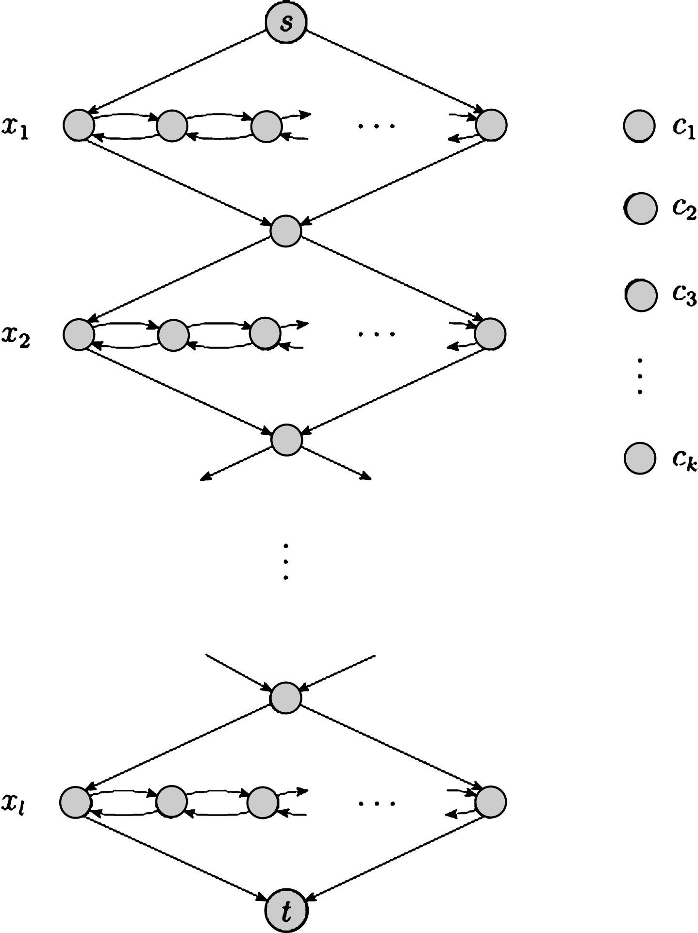
The high-level structure of G.

Fig.5

The horizontal nodes in a diamond structure.

If variable x_i appears in clause c_j, we add two edges from the jth pair in the ith diamond to the jth clause node as Fig. 6.

Fig.6

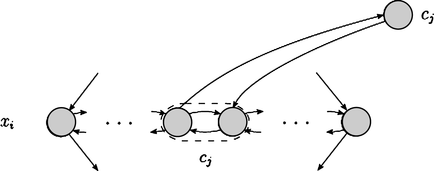
The additional edges when clause c_j contains x_i.

If ¬x_i appears in clause c_j, we add two edges from the jth pair in the ith diamond to the jth clause node, as shown in Fig. 7. We add all edges corresponding to each occurrence of x_i or ¬x_i in each clause. After assigning the appropriate degrees to the edges, the construction of G is complete. We assign weight 1 to all edges of G except edges leading from a diamond to a clause node which the diamond is corresponded to the variable that is fixed in the corresponding clause. We will describe it below.

Fig.7

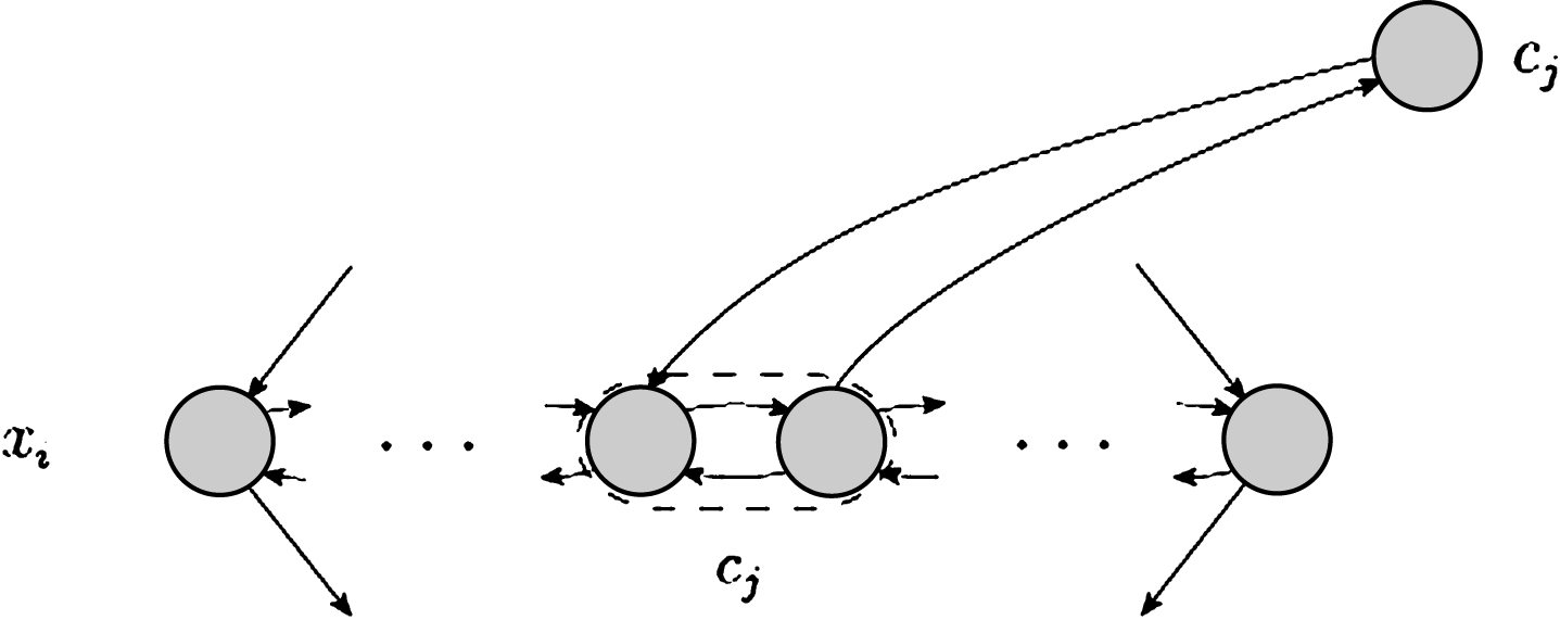
The additional edges when clause c_j contains ¬x_i.

To show that this construction works, we argue that if (φ, d) is in F3SAT, a Hamiltonian path exists from s to t with ∗-degree d and conversely if such a path exists, then (φ, d) is in F3SAT.

Suppose that there exists an assignment e to the variables of φ such that e (φ) = d. To demonstrate a Hamiltonian path from s to t with ∗-degree d, we first ignore the clause nodes. The path begins at s, goes through each diamond in turn, and ends up at t. To hit the horizontal nodes in a diamond, the path either zig-zags from left to right or zag-zigs from right to left. If a non-zero degree is assigned to x_i, the path zig-zags through the corresponding diamond. Otherwise, if x_i is assigned 0, the path zag-zigs. We show both possibilities in Fig. 8.

Fig.8

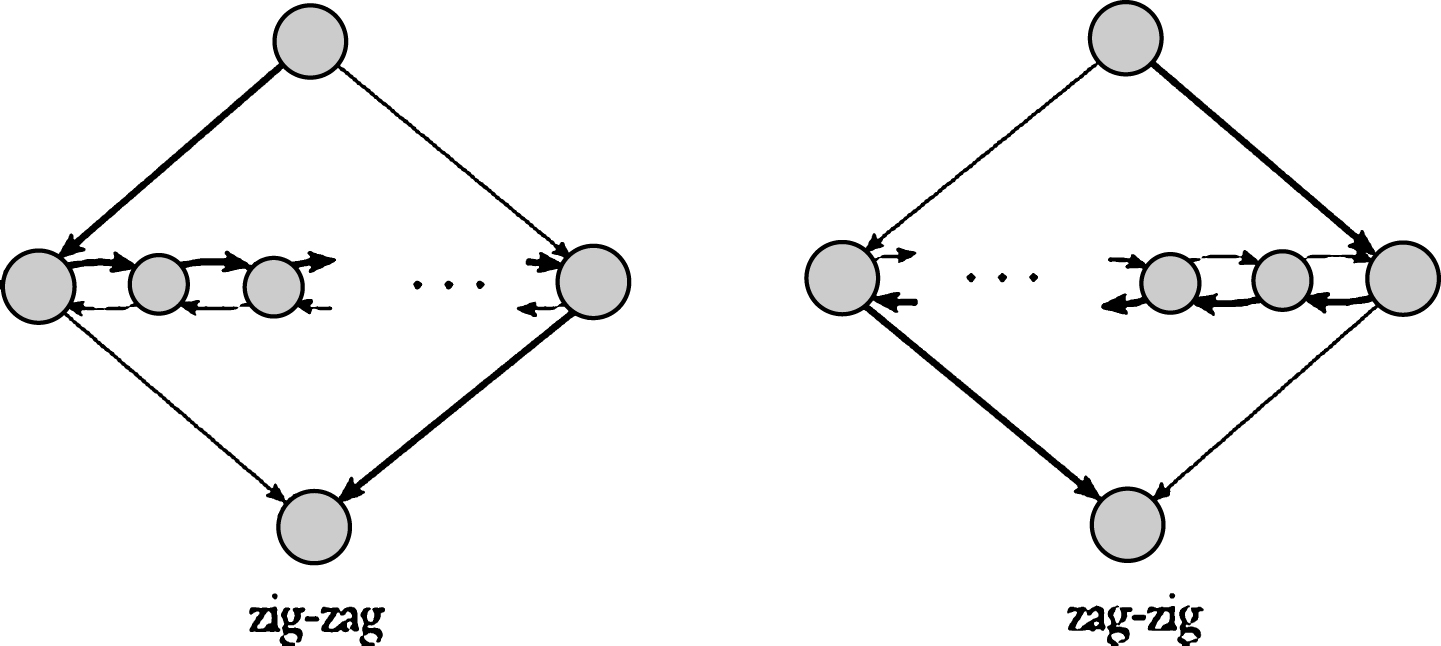
Zig-zagging and zag-zigging through a diamond, as determined by the satisfying assignment.

So far, this path covers all the nodes in G except the clause nodes. We can easily include them by adding detours at the horizontal nodes. In each clause, we select one of literals that have the maximum degree between another literals in that clause. If we selected x_i in clause c_j, we can detour at the jth pair in the ith diamond and assign degree d to the corresponding edges to/from the jth clause node. Doing so is possible because x_i must have a non-zero degree, so the path zig-zags from left to right through the corresponding diamond. Hence the edges to the node c_j are in the correct order to allow a detour. Again note that we give degree d to these detours. Similarly, if we selected ¬x_i in clause c_j, we can detour at the jth pair in the ith diamond because x_i must have degree 0, so the path zag-zigs from right to left through the corresponding diamond. Recall that since the formulas are in the language of Gödel logic, if for some variable x_i and some assignment e, we have e (x_i) =0, then e (¬ x_i) =1 is non-zero. Hence the edges to the c_j node again are in the correct order to allow a detour. Note that each literal with non-zero degree in a clause provides an option of a detour to hit the clause node. As a result, if several literals in a clause have non-zero degrees, we fix the literal with maximum degree and only one detour is taken. Thus, we have constructed the desired Hamiltonian path. Note that since all edges in obtained Hamiltonian path have degree 1 or d, so the ∗-degree of this path is d.

For the reverse direction, if G has a Hamiltonian path from s to t with ∗-degree d, we demonstrate a satisfying assignment which assign value d to φ. If the Hamiltonian path is normal; that is, it goes through the diamonds in order from the top one to the bottom one, except for the detours to the clause nodes; we can easily obtain the desired assignment. If the path zig-zags through the diamond, we assign degree d to the corresponding variable and if it zag-zigs, we assign 0. Because each clause node appears on the path, so by observing how the detour to it is taken we may determine which of literals in the corresponding clause is fixed with non-zero maximum degree. It can be easily shown that the Hamiltonian path must be normal. Also note that the proposed reduction obviously operates in polynomial time. □

6 Remarks

In this paper we have proposed a new computing model MFTM for fuzzy languages. These meta-machines have transitions with dynamic degrees corresponding with the input. The advantage of this work comparing to all previous works concerning fuzzy machines is giving explicit examples of fuzzy languages which their members have arbitrary non-crisp degrees. We studied some basic properties of these meta-machines. Next, we introduced a fuzzy theory of computational complexity and proposed two fuzzy complexity classes FP and FNP. The classes FP and FNP consist all fuzzy languages which are recognizable by deterministic or non-deterministic MFTMs, respectively. We introduced a fuzzy version of reducibility and then defined the class of FNP-complete problems. All problems in FNP are fuzzy reducible to FNP-complete problems. Moreover, we proposed some fuzzy variants of important problems in classical complexity theory such as PATH, HAMPATH, SAT and 3-SAT. We showed that PATH is in FP and FSAT, F3SAT and FHAMPATH are FNP-complete. Therefore, MFTM is a variant of Turing machine that is appropriate for studying computability and complexity properties of fuzzy languages which their elements have arbitrary degrees.

References

Bedregal

B.C.

and Figueria

, On the computing power of fuzzy Turing machines, Fuzzy Sets and Systems 159 (2008), 1072–1083.

Hajek

, Metamathematics of fuzzy logic, Kluwer, 1998.

Harkleroad

, Fuzzy recursion, ret’s and isols, Zeitschrift für Mathematische Logik und Grundlagen der Mathematik 30 (1984), 425–436.

Lee

E.T.

and Zadeh

L.A.

, Note on fuzzy languages, Information Sciences 4 (1969), 421–434.

, Fuzzy Turing machines: Variants and universality, IEEE Transactions on Fuzzy Systems 16(6) (2008), 1491–1502.

, Lattice-valued fuzzy Turing machines: Computing power, universality and efficiency, Fuzzy Sets and Systems 160 (2009), 3453–3474.

Moniri

, Fuzzy and intuitionistic fuzzy turing machines, Fundamenta Informaticae 123 (2013), 305–315.

Santos

, Fuzzy algorithms, Information and Control 17 (1970), 326–339.

Santos

, Fuzzy and probabilistic programs, Information Sciences 10 (1976), 331–335.

10.

Sipser

, Introduction to the theory of computation, Third revised edition, South-Western College Publishing, 2012.

11.

Wiedermann

, Characterizing the super-Turing computing power and efficiency of classical fuzzy Turing machines, Theoretical Computer Science 317 (2004), 61–69.

12.

Zadeh

L.A.

, Fuzzy algorithms, Information and Control 2 (1968), 94–102.