In recent advances for fuzzy dynamic modeling problem, two-stage equivalent value (EV) programming as an alternative optimization technology has been put forward to make the problem tractable in fuzzy decision-making systems. The main purpose of this paper is to provide a new methodology for computing fuzzy EV programming problem with a finite number of second-stage realizations, which is analytic and systematic rather than approximate strategy. Firstly, we provide two EV definitions in the sense of Lebesgue-Stieltjes (L-S) integral, where two L-S measures are characterized by different nondecreasing functions. Meanwhile, several properties of EV operator are presented to facilitate us to model with this operator. Secondly, for two-stage fuzzy EV programming problem, the second-stage feasibility set and fuzzy elementary feasibility set are defined. Moreover, we demonstrate the convexity of the second-stage feasibility set and recourse function, and establish the supporting hyperplane of the recourse function. Then, a new plane decomposition algorithm is developed to solve two-stage fuzzy EV programming problem, which adds iteratively feasibility and optimality cuts to the relaxed formulation of its first-stage programming problem. Finally, an illustrative example shows the solution details, and demonstrates the applicability of this proposed method.
To model random uncertainty in decision-making process, stochastic programming was proposed by Dantzig [1], Charnes and Cooper [2], which offers a rigorous methodology to formulate optimization model affected by stochasticity. Furthermore, to characterize the dynamic nature of decision-making processes in practice, two-stage stochastic programming was formulated by Dantzig [1], Beale [3], Walcup and Wets [4], in which there are two optimization problems to solved. First-stage decisions are taken in the presence of stochastic uncertainty. In the second stage, recourse problem arises to perform the corrective actions where the recourse decisions (second-stage decisions) are taken after observing the realizations of random parameters. The coefficient matrix of the recourse decision vector is referred to as recourse matrix, which characterizes the feature of the recourse problem. However, the first-stage decisions are chosen by taking the future effects into account. Therefore, recourse function is employed to measure the future effects which is expressed by computing the expected value of the second-stage value function.
On account of solving two-stage stochastic programming by analytic method, L-shaped method based on cutting plane technology was developed by Van Slyke and Wets [5], which is one kind of Benders decomposition [6] and includes two main frameworks: feasibility cut and optimality cut. For instance, Marti [7] modeled the plastic design problem of mechanical structures as a two-stage stochastic linear programming with complete fixed recourse, and solved it by the L-shaped decomposition method. Two-stage stochastic linear programming is usually used to model the resilience system [8]. For other features of two-stage stochastic linear programming, the interested reader may refer to the books [9, 10] and the references therein.
Taking into account fuzzy uncertainty, fuzzy programming problems have been widely studied by many academic researchers. Baykasoglu and Gocken [11] presented a review of fuzzy mathematical programming models. Based on fuzzy theory [12, 13], many fuzzy programming problems were proposed, such as fuzzy multi-objective programming [14, 17], two-stage robust integer programming [15], supplier management [16], supply chain network design [18]. Credibility theory is a mathematical tool to deal with subjective uncertainty, it has been widely used in the literature, the interested reader may refer to [19, 20]. Within the framework of credibility theory, robust/reliability based optimization [21], p-hub center problems [22], fuzzy value-at-risk (VaR) optimization model [23], and location-routing problems [24] were formulated by researchers.
To cope with fuzzy dynamic modeling problem, Liu [25] firstly proposed two-stage fuzzy programming problem. Several examples of such two-stage programming problem with fuzzy variable can be found in fuzzy random programming with recourse [26], recourse-based facility-location problem [27], geometric programming problem [28], and uncapacitated hub location problem with recourse [29]. For the general two-stage fuzzy programming problems, due to the lack of linearity on fuzzy expected value operator, recourse function could not maintain the convexity of the second-stage value function. Then, cutting plane method could not apply directly to two-stage fuzzy programming due to recourse function without the desirable convexity. Therefore, two-stage fuzzy programming problems were usually solved by heuristic algorithms. Despite the considerable effects to solve two-stage fuzzy programming by many researchers through heuristic algorithms, the analytic solution method is also required urgently to solve this programming problem with accuracy and more efficiency.
The aim of this paper is to develop an analytic solution method based on plane decomposition to solve two-stage fuzzy programming problems. To the best of our knowledge, this issue has not yet been studied in two-stage fuzzy programming literatures. Taking advantage of credibility theory and L-S integral [30, 31], we show the formulation of two-stage fuzzy EV programming, discuss its properties, and then develop a new plane decomposition algorithm for solving this two-stage programming problem. The contributions of this study are summarized as three aspects:
We provide two EV definitions by means of L-S integral, and basic properties as well as Cauchy-Schwarz inequality on EV operator.
For two-stage fuzzy EV programming problem, we first show the convexity of the second-stage value function and recourse function.
A new plane decomposition algorithm is proposed, which is adapt to two-stage fuzzy EV programming problem.
The remainder of paper is structured as follows. Section 2 provides two EV definitions by two different L-S measures, and discusses on the properties of EV operator. Section 3 focuses on two-stage fuzzy EV programming problem. Section 4 develops a new plane decomposition algorithm for solving this two-stage fuzzy programming problem. An application example is conducted in Section 5. Finally, Section 6 gives the conclusions.
L-S integral and EV
Combing with Lebesgue measure theory, L-S integral is developed on the basis of Riemann-Stieltjes integral which is produced for integrating one function with respect to another function. L-S integral is a powerful integration method especially in probability theory. We refer to the books [30, 31] for details on L-S integral and the references therein.
L-S integral is a class of linear integral with respect to L-S measure. By L-S integral, we can formulate the EV definitions of fuzzy variable and fuzzy variable’s function. Under different L-S measures generated by two types of nondecreasing functions, we will provide two definitions of EV to demonstrate the relation between L-S measure and EV.
Case I: Univariate Integral
Let be a credibility space, where Γ a universe, is the power set of Γ and Cr is a set function defined on . Suppose that ξ is a fuzzy variable defined on credibility space , and the monotone nondecreasing function of fuzzy variable ξ is usually defined as . Then we define the L-S α-Measure μα (I) of interval I with end points a, b as follows
where .
Definition 1. Let ξ be a fuzzy variable with nondecreasing function α (·), and f (x) a real-value function on . Then the EV of fuzzy variable function f (ξ) is defined as
Specially, in the case that f (x) = x, the EV of fuzzy variable ξ can be achieved by
In particular, when ξ is a discrete fuzzy variable with realizations , its monotone nondecreasing function α (t) is formulated as a left-continuous step function. Then
Example 1. Let ξ be a discrete fuzzy variable with following possibility distribution:
Firstly, calculate the monotone nondecreasing function of fuzzy variable ξ,
Then
Case II: Multivariate Integral
We now turn to show the EV definition of fuzzy variable’s function with more than one fuzzy variables, and adopt product measure α1 × α2 × ⋯ × αn-measure as the L-S measure to construct L-S integral.
Let ξi, i = 1, 2, …, n be fuzzy variables defined on a credibility measure space . For each i, the monotone nondecreasing function of fuzzy variable ξi is computed by . Let μαi be the L-S α-measure generated by monotone nondecreasing function αi (·), then we define the L-S α1 × α2 × ⋯ × αn-measure of the polyhedron I1 × I2 × ⋯ × In, denoted by μα1×α2×⋯×αn, and
Definition 2. Let ξi be a fuzzy variable with monotone nondecreasing function αi (·) for i = 1, 2, …, n respectively, and f (x1, x2, …, xn) a real-value function on . Then the EV of the function f (ξ1, ξ2, …, ξn) is defined as
For more details about L-S measure generated by joint nondecreasing function, the interested reader may refer to [32].
In the case that ξ1, ξ2, …, ξn are discrete fuzzy variables with monotone nondecreasing function αi (·), i = 1, 2, …, n, respectively, we employ a fuzzy vector ξ, which is constructed by ξ1, ξ2, …, ξn and can be represented as ξ = (ξ1, ξ2, …, ξn) with realizations for k = 1, 2, …, K and K = N1 × N2 × ⋯ × Nn, where Ni is the number of realizations of fuzzy variable ξi for i = 1, 2, …, n. Then, according to Definition 2, the EV of f (ξ) = f (ξ1, ξ2, …, ξn) can be computed as
For the sack of simplicity, we employ the notation Δα (·) to denote the variation of the joint monotone nondecreasing functions α1 × α2 × ⋯ × αn at each realization , k = 1, 2, …, K, i.e.,
Then, the EV of f (ξ) can also be rewritten as
According to the above EV definitions, we can deduce several properties of EV operator as follows.
Proposition 1.Let ξ and η be fuzzy variables, we have
(Normality) If ξ ≥ 0, then E [ξ] ≥0;
(Linearity) For any real numbers a, b,
(Monotonicity) If ξ ≥ η, then E [ξ] ≥ E [η];
(Convexity) If f (x, ξ) is a convex function on , then E [f (x, ξ)] is also a convex function.
Proof. i) The assert i) holds obviously.
ii) 1o. Let ξ and η be discrete fuzzy variables with realizations and , and nondecreasing functions α1, α2 correspond to fuzzy variables ξ and η respectively, then
On the other hand, according to Definition 2, we have
The above equation holds due to the fact that
2o. If ξ and η be non-negative continuous fuzzy variables, there exist two discrete fuzzy variable sequences {ξn} and {ηn} such that ξn ↑ ξ, ηn ↑ η, and E [aξn + bηn] = aE [ξn] + bE [ηn]. Let n→ ∞, then assert ii) also holds in this case.
3o. When ξ and η are arbitrary continuous fuzzy variables, then they can be denoted as ξ = ξ+ - ξ- and η = η+ - η-, where ξ+ = max {ξ, 0} and ξ- = - min {ξ, 0}. Note that ξ+, ξ-, η+, η- are non-negative continuous fuzzy variables.
iii) If ξ ≥ η, then ξ - η ≥ 0. It follows from assert i) and assert ii) that E [ξ - η] = E [ξ] - E [η] ≥0, then assert iii) holds.
iv) It follows from asserts ii) and iii) that assert iv) holds. In fact, for fixed ξ, arbitrary and λ ∈ [0, 1], we have
then
This completes the proof. □
Then, we provide the relation on EV operator, which is referred as to Cauchy-Schwarz inequality, and show the upper bound of EV of product of two fuzzy variables.
Proposition 2.(Cauchy-Schwarz inequality) Let ξ and η be fuzzy variables and ξ · η ≠ 0, we have
Proof. Firstly, we have E [ξ2] >0 and E [η2] >0. Let , , then
Taking EV operator E [·] to the both sides of the above inequality, then , it follows that Cauchy-Schwarz inequality holds. The proof is now completed. □
Formulation of two-stage fuzzy EV programming
By means of EV operator, we can formally present a generic two-stage EV programming problem with fixed recourse, which can be formulated as follows,
where , E [·] is the EV operator, and
In the above formulation, we usually refer to Q (x, ξ) as the second-stage value function, and is called as recourse function, which is equal to the EV of Q (x, ξ). The first-stage decision is represented by the vector x = (x1, x2, …, xn1) T, while the second-stage decision is represented by y = (y1, y2, …, yn2) T. The technology matrix A and recourse matrix W are known matrices of sizes m1 × n1 and m2 × n2 respectively, c and b are known vectors in and respectively. For each γ ∈ Γ, , , and T (γ) is an m2 × n1 matrix (T1 (γ) , T2 (γ) , … , Tn1 (γ)), where Ti (γ) is the i-th column of matrix T (γ) for i = 1, 2, …, n1. Therefore, we obtain a fuzzy vector ξ = (q (γ) T, h (γ) T, T1 (γ) T, T2 (γ) T, … , Tn1 (γ) T) with n2 + m2 + n1 × m2 components. The decisions x are here-and-now (or first-stage) decisions that are taken before the realizations of the fuzzy parameter ξ is known, whereas the wait-and-see (or second-stage) decisions y can adapt to the realization of ξ.
Remark 1. Suppose that fuzzy vector ξ is constructed by discrete fuzzy variables ξ1, ξ2, … , ξn, and each fuzzy variable ξi possesses a monotone nondecreasing function αi (·). Then, according to Definition 2, the value of recourse function at x can be computed by the formula
where each realization can also be stated as . Meanwhile, for each , the second-stage value function can be obtained from the following programming problem
Let K1 = {x ∣ Ax = b} be the set determined by the technology matrix A, and the set does not depend on the particular realization of fuzzy vector ξ. Let K2 be the second-stage feasibility set, which can be stated as . All elements in K2 are those decisions x for which the second-stage problem has a feasible solution for almost every realization or scenario . Let Ξ be the support of fuzzy vector ξ, i.e., the smallest closed subset in such that Cr {γ ∣ ξ (γ) ∈ Ξ} =1. The deterministic equivalent programming problem of this two-stage EV programming problem can be rewritten as
Next, we will turn to demonstrate several theorems, which play an important role in the proposed decomposition algorithm. At first, to facilitate us to clarify the problem, define a set
which is referred to as “fuzzy elementary feasibility set”. In the following, we demonstrate the convex property of the second-stage feasibility set K2 through fuzzy elementary feasibility set K2 (ξ (γ)) under mild conditions.
Theorem 1.i) For a given fuzzy vector ξ, the fuzzy elementary feasibility set K2 (ξ (γ)) is a convex polyhedron;
ii) When ξ is a finitely discrete fuzzy vector, K2 is a convex polyhedron.
Proof. i) Let x1, x2 ∈ K2 (ξ), and Wy1 = h (γ) - T (γ) x1, Wy2 = h (γ) - T (γ) x2, then . Due to y1 + (1 - λ) y2 ≥ 0, then K2 (ξ (γ)) is a convex set.
Let posW = {t ∣ Wy = t, y ≥ 0} be a convex set. Now, we prove the polyhedron K2 (ξ (γ)) by the set posW. Consider some x and ξ (γ), it follows from x ∈ K2 (ξ (γ)) that h (γ) - T (γ) x ∈ posW. If no y ≥ 0 exists such that Wy = h (γ) - T (γ) x, i.e. "x ∉ K2 (ξ (γ)) ⇔ some x and ξ (γ) such that h (γ) - T (γ) x ∉ posW". Then, there exists a point h (γ) - T (γ) x, which does not belong to the convex set posW. By the separation theorem of convex sets, there must exist some hyperplanes {x ∣ σTx = 0} that separate h (γ) - T (γ) x from posW. These hyperplanes satisfy σTx ≤ 0 for x ∈ posW and σ [h (γ) - T (γ) x] >0. Because recourse matrix W is fixed, there are only finitely many different such hyperplanes. Combining the above two conclusions, K2 (ξ (γ)) is a convex polyhedron.
ii) When ξ is a finitely discrete fuzzy vector, then
the intersection of finitely many convex polyhedron is also a convex polyhedron. The proof is now completed. □
Theorem 2.For arbitrary fuzzy vector ξ with the condition that E [ξ2]< ∞, then K2 = ⋂ ξ∈ΞK2 (ξ (γ)) and K2 is a convex set.
Proof. For ∀ x ∈ K2, then Cr {γ ∣ Q (x, ξ) < ∞} =1. On the other hand Cr {γ ∣ ξ (γ) ∈ Ξ} =1. We have
which is a closed set of {γ ∣ ξ (γ) ∈ Ξ} with credibility 1. Thus, Cr {γ ∣ ξ (γ) ∈ Ξ, Q (x, ξ) < ∞} =1 and {γ ∣ ξ (γ) ∈ Ξ} = {γ ∣ ξ (γ) ∈ Ξ, Q (x, ξ) < ∞}. Then {ξ ∣ Q (x, ξ) < ∞} ∈ Ξ. Therefore, x ∈ ⋂ ξ∈Ξ {x ∣ Q (x, ξ) < ∞}, K2 ⊆ ⋂ ξ∈ΞK2 (ξ (γ)) .
For ∀ x ∈ ⋂ ξ∈ΞK2 (ξ (γ)), and a fixed ξ, solving the programming problem (2), we can finding an optimal basis B which is a square submatrix of W, and Q (x, ξ) can be computed by Q (x, ξ) = qB (γ) TB-1 (h (γ) - T (γ) x) where qB (γ) is the subvector of q (γ) associated to the optimal basis B. Then, the recourse function can be rewritten as . Due to the condition that E [ξ2]< ∞, then
According to Cauchy-Schwarz inequality of Proposition 2, we have . Therefore, x ∈ K2 and ⋂ξ∈ΞK2 (ξ (γ)) ⊆ K2. We conclude that K2 = ⋂ ξ∈ΞK2 (ξ (γ)) in this case. It follows from assert i) of Theorem 1 that K2 (ξ) is a convex set, then K2 is also a convex set. This completes the proof. □
In the following, we will demonstrate the convexity of second-stage value function Q (x, ξ) and recourse function , and show that recourse function is a convex polyhedral function on K2.
Theorem 3.i) For a given fuzzy vector ξ, the second-stage value function Q (x, ξ) is a piecewise linear function, and Q (x, ξ) and recourse function are convex functions on K2;
ii) When ξ is a finitely discrete fuzzy vector with realizations , then is a piecewise linear function on K2.
Proof. i) Let B be the optimal basis of the programming problem (2), then Q (x, ξ) = qB (γ) TB-1 (h (γ) - T (γ) x) which is linear in x on K2. Due to the fact that second-stage programming problem (2) exists finitely different optimal bases, it follows that the value function Q (x, ξ) is a piecewise linear function for all x ∈ K2.
Let x1, x2 ∈ K2 and be the optimal solutions to the second-stage programming problem (2) corresponding to x1, x2 respectively, then . On the other hand, for λ ∈ [0, 1],
We know that is a feasible solution to the above programming problem, let y* be an optimal solution of this problem, then
Therefore, Q (x, ξ) is a convex function. By the assert iv) of Proposition 1, we know that is also a convex function.
ii) When ξ is a finitely discrete fuzzy vector with realizations , then
According to the above proof, the second-stage value function is a piecewise linear convex function in x, and , the linear summation of finite function is also a piecewise linear function in x on K2. The proof of theorem is now completed. □
Theorem 4.Let ξ be a discrete fuzzy vector with realizations for k = 1, 2, …, K. Let denotes the optimal simplex multiplier corresponding to the solution to the second-stage programming problem (2) with and realization , then , and is a support of the recourse function .
Proof. For the realization , the dual programming of second-stage programming problem (2) can be stated as
Since is the optimal simplex multiplier for the second-stage programming problem (2) with , according to the duality theory, we have
Because the constraints of dual programming (5) are independent of x, is a feasible solution to dual programming (5) for all x ∈ K2. Let πk be the optimal solution to dual programming (5) corresponding to x, then
By multiplying to the both sides of the above inequality, then
Taking summation from k = 1 to K, we have
which completes the proof of theorem. □
Theorem 5.Suppose that is finite on K2, and ξ is a finitely discrete fuzzy vector with realizations . Then is a convex polyhedral function.
Proof. By letting x range over K2, we know that only a finite number of supports
of can be generated, since each corresponds to an optimal basis B, which is a square submatrix of W. Moreover, recourse matrix W has only a finite number of square submatrices. On the other hand, for all , there exists a support which satisfies that
Therefore, the upper envelope of this finite number of linear supports coincides with . This completes the proof. □
These theorems above devote theoretical foundation to algorithm analysis, and play a key role in formulation of plane decomposition algorithm.
Description of algorithm
First of all, we provide the equivalent representation of programming problem (4) as follows
The analytic solution method based on plane decomposition solves the two-stage EV programming problem by considering that each scenario is independent and therefore the prime problem structure can be decomposed into a master problem (a relaxed formulation of the first-stage programming problem) and a number of subproblems to speed up the solution time. The decisions of these subproblems are linked to the master problem through the approximation θ of objective function of the second-stage programming problems. At the first iteration, θ is set to zero. Then, two main frameworks are used, one is feasibility cut and another is optimality cut, which add iteratively to the master problem of fuzzy EV programming problem. Therefore, the master problem will be updated by introducing new cut constraints at each iteration. This algorithm proceeds as follows:
Set r = s = v = 0.
Set v = v + 1. Solve the linear programming problem
The definitions of these parameters Dl, dl, El and el are given in the following steps. θv is set equal to -∞ and is not considered in computation of xv.
(Feasibility Cut) Check if . For given xv determined by Step 1, and every realization for k = 1, 2, …, K, solve the linear programming problem
where e = (1, 1, …, 1). Then, we explore an analysis to the optimal value of programming problem (8):
1o. For some realizations , the optimal value w1 > 0, then let be the associated dual simple multiplier, and
Generating a feasibility cut as the second constraint of programming problem (7):
Set r = r + 1 and return to Step 1.
2o. For all realizations , k = 1, 2, …, K, all the corresponding optimal values are w1 = 0, then xv ∈ K2. Go to Step 3.
(Optimality Cut) For given xv determined by Step 1 and Step 2, and every realization from k = 1 to K, the dual problem of the second-stage programming problem (3) is formulated as:
where π = (π1, π2, …, πm2). Then we can obtain the optimal simplex multiplier corresponding to xv and . Let
and . If , stop. Then xv is an optimal solution. If , generating an optimality cut as the third constraint of programming problem (7):
or
Set s = s + 1 and return to Step 1.
Remark 2. In Step 3, we usually add the checking process on before deciding to carry on this step to obtain the optimal simplex multiplier of xv with respect to . In fact, if , then the terms and are also equal to zero. These two terms have no effect on es+1 and Es+1 respectively. Based on this fact, Step 3 only requires us to consider the optimality of any solution xv with respect to .
In order to illustrate the convergence of the algorithm, we now reasonable demonstrate that the algorithm will converge to the optimal solution at most a finite number of iterations.
Theorem 6.When two-stage fuzzy EV programming problem has a finite number of second-stage realizations, the plane decomposition algorithm applying to this programming problem converges to the optimal solution after finite iterations.
Proof. At first, we now prove that a finite number of feasibility cuts are generated to guarantee xv ∈ K2. In Step 2, a necessary condition for xv ∈ K2 is that
On the one hand, there are only a finite number of optimal bases (the basis of W) solved in Step 2. On the other hand, it follows from Theorem 1 that the second-stage feasible set K2 is a convex polyhedron when ξ is a finitely discrete fuzzy vector. Then we conclude that this algorithm can obtain a feasible solution as long as a finite number of such feasibility cuts exist in Step 2.
We then prove that at most finitely many optimality cuts are required to convergence to the optimal solution in Step 3. For the solution xv, the second-stage programming problem is solved repeatedly for each k = 1, 2, …, K, yielding optimal simplex multipliers . If (xv, θv) is optimal for programming problem (6), it follows that . Then, according to Theorem 4, this happens
which justifies the termination criterion in this step. If (xv, θv) is not optimal, then . Therefore, a new optimality cut
or
is generated. Because each corresponds to one basis of programming problem (3), and there are only a finite number of different combinations of the K multipliers , then this programming problem converges to the optimal solution after finite optimality cuts. This completes the proof. □
Case study
For clearly showing the solution process of the proposed algorithm, we carry out a numerical example to demonstrate the applicability of the proposed decomposition algorithm. The data of model are stated as follows
where ξ and η are discrete fuzzy variables with the following possibility distributions
Meanwhile, the monotone nondecreasing functions α1, α2 corresponding to two fuzzy variables ξ and η can be stated as
Then, fuzzy vector
is constructed by discrete fuzzy variables ξ and η, which is a discrete fuzzy vector with the following realizations ,
In this case, for the realization ,
Due to this fact, for a given feasible solution xv, we need only to check the optimality of solution xv with respect to , and .
In the following, we turn to solve the two-stage fuzzy EV programming problem to show the iteration process of plane decomposition algorithm.
The First Iteration:
Set r = s = v = 0.
Solve the following linear programming problem
the optimal solution is x1 = (0, 2.5) T, and set θ1 = -∞.
We check the feasibility of the solution x1 = (0, 2.5) T by solving the programming problem (8) with respect to . When , the optimal value of the programming problem (8) is w1 = 1 >0. Thus, x1 = (0, 2.5) T is infeasible. Let be the associated dual simple multiplier (-1, 0.5), then . Generating a feasibility cut D1x ≥ d1, i.e.,
Add it to the constraints of the programming problem (11) and begin to the Second Iteration.
The Second Iteration:
We obtain the following programming problem by the first iteration:
whose the optimal solutions are θ2 = -∞ and x2 = (0.6667, 2.1667) T.
Substituting x2 into programming problem (8), solving the corresponding programming problem with respect to , and respectively, we obtain all the optimal values are w1 = 0. Thus, x2 = (0.6667, 2.1667) T is a feasible solution for the second-stage problem.
Due to the fact that θ2 = -∞, it is non-optimal. Solving the dual problem (9) for , respectively, and the corresponding optimal solutions are , , and respectively. Let
Generating an optimality cut E1x + θ ≥ e1, i.e.,
Adding the optimality cut into the programming problem (12) and starting the Third Iteration.
The Third Iteration:
We obtain the following programming problem
Solving the above problem, we gain the optimal solutions are x3 = (5, 0) T and θ3 = 1.9.
Checking the feasibility of x3 = (5, 0) T by the programming problem (8) for , and respectively. When , the optimal solution of programming problem (8) is w1 = 2.5 > 0. Thus, the solution x3 = (5, 0) T is infeasible. Let be the associated dual simple multiplier (0.5, - 1), then . Generating a feasibility cut D2x ≥ d2, i.e.,
Add it to the constraints of programming problem (13) and turn to the Forth Iteration.
The Forth Iteration:
We obtain the following programming problem
whose the optimal solutions are θ4 = 5.0667 and x4 = (3.3333, 0.8333) T.
Substituting x4 into programming problem (8). By solving the programming problem with respect to , and respectively, we obtain all the optimal values are w1 = 0. Therefore, the solution x4 = (3.3333, 0.8333) T is a feasible solution to the second-stage problem.
Checking the optimality of the solution (x4, θ4). For x = x4, solving the dual problem (9) for , respectively, and the corresponding optimal solutions are , , and . Then, e2 = 1.975, E2 = (-0.05, - 3.75). We have
Therefore, generating an optimality cut E2x + θ ≥ e2, i.e.,
Adding the optimality cut into the programming problem (14) and starting the Fifth Iteration.
The Fifth Iteration:
We obtain the following programming problem from the above iterations,
Solving the above programming problem, and we obtain the optimal solutions are θ5 = 5.2667 and x5 = (3.3333, 0.8333) T.
Checking the feasibility of the solution x5 = (3.3333, 0.8333) T. Since x5 = x4, it is also a feasible solution to the second-stage problem. In the following, we check if (x5, θ5) is the optimal solution to the prime problem.
Similarly, due to x5 = x4, the dual problem of the second-stage programming problem is same to those in the Forth Iteration for respectively. Therefore, the dual problems have the same optimal solutions , , and respectively. Then, e3 = e2 = 1.975, E3 = E2 = (-0.05, - 3.75), and e3 - E3 · x5 = 5.2667 = θ5. Thus, (x5, θ5) is the optimal solution, and the iteration is stopped.
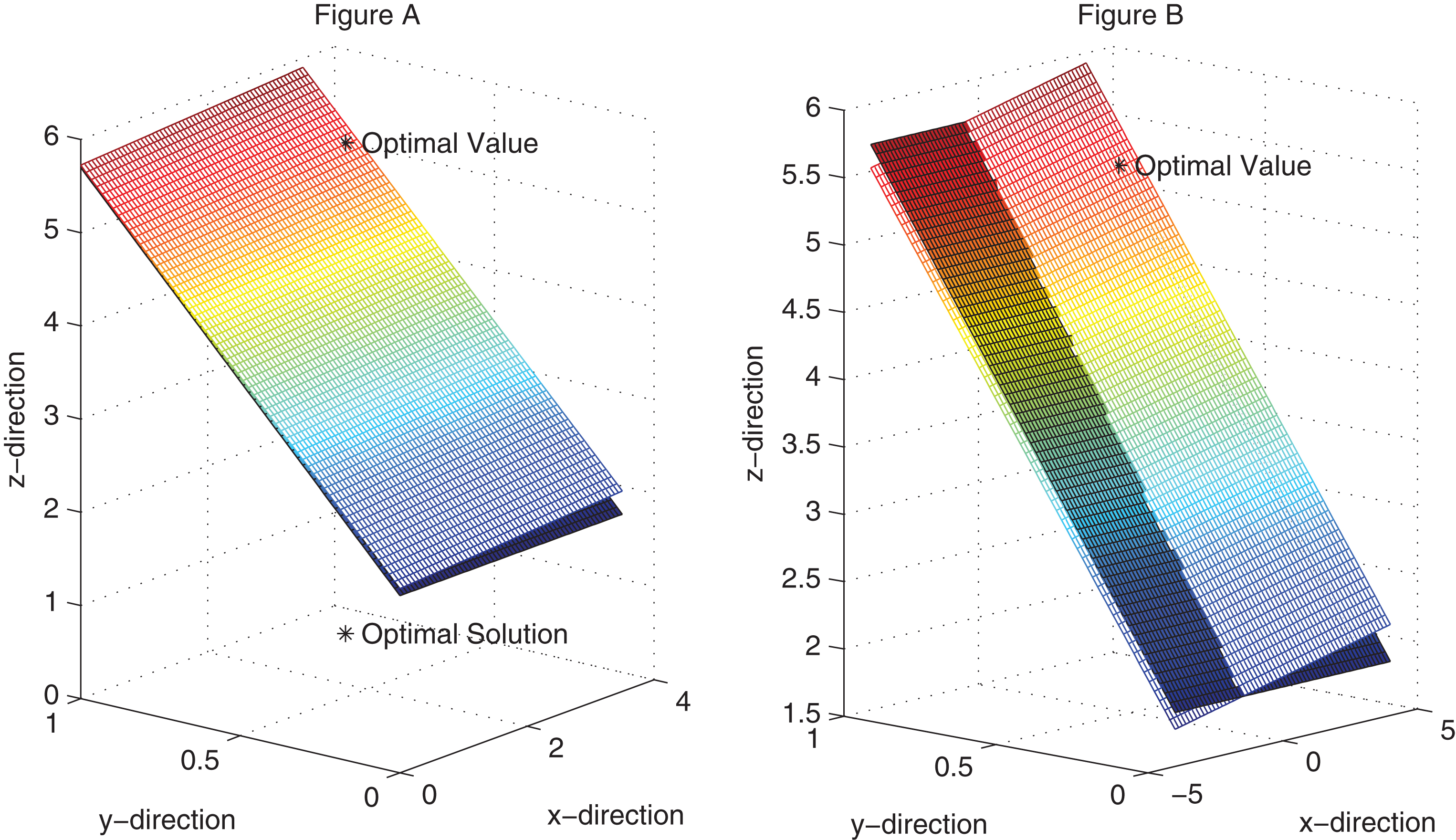
To clearly illustrate the relation between the optimality cuts and the optimal solution (x5, θ5), two graphs are plotted in Fig. 1. Two supporting hyperplanes of recourse function are generated by two optimality cuts -3.8x2 + θ ≥ 1.9 and -0.05x1 - 3.75x2 + θ ≥ 1.975, the first one is the hyperplane {(x, y, z) ∣ z - 3.8y = 1.9}, and the second hyperplane is {(x, y, z) ∣ z - 0.05x - 3.75y = 1.975}. The left graph shows that the optimal value corresponding to the optimal solution (x5, θ5) = (3.3333, 0.8333) is generated by the second hyperplane {(x, y, z) ∣ z - 0.05x - 3.75y = 1.975}. The right graph expresses the intersection of these two supporting hyperplanes on the whole x-direction.
Optimality cuts and the optimal value.
From the above iteration processes, we obtain that the optimal solution of two-stage EV programming problem is x* = (3.3333, 0.8333) T, and the corresponding optimal value of the whole programming problem is 12.7667.
Conclusions
In this paper, a new algorithm has been set out to solve two-stage fuzzy EV programming problem by feasibility cuts and optimality cuts. The obtained results included the following aspects: (i) Two EV definitions were presented, and the properties and Cauchy-Schwarz inequality on EV operator were developed; (ii) The second-stage feasibility set and fuzzy elementary feasibility set were defined. Furthermore, we demonstrated the convexity of the second-stage value function and recourse function; (iii) A new plane decomposition algorithm was proposed, and a computational experiment was conducted to illustrate the effectiveness of the proposed decomposition algorithm.
Footnotes
Acknowledgments
This research was supported by the National Natural Science Foundation of China (Nos. 51675026, 71671009), and the National Basic Research Program of China (No. 2013CB733002).
References
1.
DantzigG.B., Linear programming under uncertainty, Management Science1 (1955), 197–206.
2.
CharnesA. and CooperW.W., Chance-constrained programming, Management Science6 (1959), 73–79.
3.
BealeE.M.L., On minimizing a convex function subject to linear inequalities, J. Royal Statistical Society(Series B)17 (1955), 173–184.
4.
WalcupD.W. and WetsR., Stochastic programs with recourse, SIAM Journal of Applied Mathematics15 (1967), 1299–1314.
5.
Van SlykeR. and
WetsR.J.-B., L-shaped linear programs with application to optimal control and stochastic programming, SIAM Journal on Applied Mathematics17(4) (1969), 638–663.
MartiK., Optimal structural design under stochastic uncertainty by stochastic linear programming methods, Reliability Engineering & System Safety72 (2001), 165–177.
8.
HosseiniS., BarkerK. and Ramirez-MarquezJ.E., A review of definitions and measures of system resilience, Reliability Engineering & System Safety145 (2016), 47–61.
9.
KallP. and MayerJ., Stochastic Linear Programming: Model, Theory and Computation, Springer, New York, 2005.
10.
BrigeJ.R. and LouveauxF., Introduction to Stochastic Programming, Springer, New York, 2011.
11.
BaykasogluA. and GockenT., A review and classification of fuzzy mathematical programs, Journal of Intelligent & Fuzzy Systems19 (2008), 205–229.
12.
ZadehL.A., Fuzzy sets, Information and Control8 (1965), 338–353.
13.
ZadehL.A., Fuzzy sets as a basis for a theory of possibility, Fuzzy Sets and Systems1 (1978), 3–28.
14.
PalB.B. and MoitraB.N., A goal programming procedure for solving problems with multiple fuzzy goals using dynamic programming, European Journal of Operational Research144 (2003), 480–491.
15.
LiY.P., HuangG.H., NieX.H. and NieS.L., A two-stage fuzzy robust integer programming approach for capacity planning of environmental management systems, European Journal of Operational Research189 (2008), 399–420.
16.
AminS.H. and RazmiJ., An integrated fuzzy model for supplier management: A case study of ISP selection and evaluation, Expert Systems with Applications36 (2009), 8639–8648.
17.
TangJ., PanZ., FungR.Y.K. and LauH., Vehicle routing problem with fuzzy time windows, Fuzzy Sets and Systems160 (2009), 683–695.
18.
KristiantoY., GunasekaranA., HeloP. and HaoY., A model of resilient supply chain network design: A two-stage programming with fuzzy shortest path, Expert Systems with Applications41 (2014), 39–49.
19.
LiuB. and LiuY.K., Expected value of fuzzy variable and fuzzy expected value models, IEEE Transactions on Fuzzy Systems10(4) (2002), 445–450.
QuarantaG., Finite element analysis with uncertain probabilities, Computer Methods in Applied Mechanics and Enginering200 (2011), 114–129.
22.
YangK., LiuY.-K. and YangG.-Q., Solving fuzzy-hub center problem by genetic algorithm incorporating local search, Applied Soft Computing13 (2013), 2624–2632.
23.
BaiX. and LiuY., Robust optimization of supply chain network design in fuzzy decision system, Journal of Intelligent Manufacturing27 (2016), 1131–1149.
24.
WeiM., YuL. and LiX., Credibilistic location-routing model for hazardous materials transportation, International Journal of Intelligent Systems30 (2015), 23–39.
25.
LiuY.-K., Fuzzy programming with recourse, International Journal of Uncertainty, Fuzziness and Knowledge-Based Systems13(4) (2005), 381–413.
26.
LiuY.-K., The approximation method for two-stage fuzzy random programming with recourse, IEEE Transactions on Fuzzy Systems15(6) (2007), 1197–1208.
27.
WangS., WatadaJ. and PedryczW., Recourse-based facilitylocation problems in hybrid uncertain environment, IEEE Transactions on Systems, Man, and Cybernetics–Part B: Cybernetics40(4) (2009), 1176–1187.
28.
ChakrabortyD., Solving geometric programming problems with fuzzy random variable coefficients, Journal of Intelligent & Fuzzy Systems28 (2015), 2493–2499.
29.
ZhaiH., LiuY.-K. and YangK., Modeling two-stage UHL problem with uncertain demands, Applied Mathematical Modelling40 (2016), 3029–3048.
30.
CarterM. and van BruntB., The Lebesgue-Stieltjes Integral: A Practical Introduction, Springer-Verlag, New York, 2000.