Fuzz-iDEVS: An approach to model imprecisions in Discrete Event Simulation

Abstract

In this work, we present a discrete event model that incorporates the lack of precision of variables. The make use of Fuzzy Set Theory to generate the model, and apply it on fire propagation study case. Our aim is to propose a generalization to the discrete event system specification formalism (DEVS) which be able to deal with imprecision in all of its elements (events, transition functions, state). Our approach is based on mathematical definitions of the Fuzzy Set Theory to represent and use imprecise information in the DEVS formalism.

Keywords

Discrete Event Simulation discrete event system DEVS fuzzy set theory fuzzy logic

1 Introduction

Theory of Modeling and Simulation (TMS) [48] has emerged as an essential tool for analyzing the behavior of complex dynamic systems. Modeling can be defined as an operation by which the model of a complex system is established during an analysis process, or put into an equation in order to obtain a simplified, interpretable and simulable representation of it. Discrete Event Simulation (DES [14]) is often used to simulate complex systems. They are modeled by sequences of events recording significant qualitative changes in the state of the system. Actually, DES is widely used in many technological and engineering systems, such as communication networks, computer networks, manufacturing systems, transportation systems, natural systems, and many more. Many formal foundation modeling approaches of DES have been proposed and developed, including the notably Petri nets, Cellular Automata, etc.

Discrete EVent system Specification (DEVS) [48] is a popular formalism for modeling complex dynamic systems using a discrete-event abstraction. At this abstraction level, a timed sequence of pertinent (external) events input to a system (or internal, in the case of timeouts) cause instantaneous changes to the state of the system. Main advantages of DEVS are its rigorous formal definition, and its support for modular composition.

DEVS is also defined as a multi-formalism [42]. It can be used to include or describe other types of formalism. In this work, we are interested in the Fuzzy Set Theory in order to extend the capacity of the DEVS formalism to model and handle imprecise data. This article proposes a synthesis of several works based on Fuzzy Set Theory (FST) [5 , 11] and Fuzzy Inference Systems (FIS) [2–4 , 25].

The first section describes the theoretical frame of our work: Discrete Event Systems (DES) and the Theory of Modeling and Simulation (TMS). The second section presents our imprecise modeling approach, in particular as we propose to integrate the concepts of the Fuzzy Set Theory (FST) into the DEVS formalism. The third section deals with the representation of Fuzzy Inference System (FIS) in the DEVS formalism. Before conclude, the last section quickly presents several applications and above all a model of Fires propagation.

2 Discrete Event Systems: DES

In DES, the model is represented as a discrete-state, event-driven dynamic structure. The space is described by a discrete set and the states evolve in terms of asynchronous occurrence of discrete events over time [14]. States, events and transition functions have discrete values and they are defined as a five-tuple [14 , 33]. A Discrete Event model is a structure: $G = (S, Σ, δ, λ, s_{0}),$ (1) where:

S: is the set of states and Q = {(s, t_e) |s ∈ S, t_e ∈ (T)} is the set of total states, t_e is the elapsed time since the last event and T the base time;

Σ: is the set of events containing detectable (an event is detectable if it produces a measurable change in the system output) and undetectable events, which are generally fired asynchronously;

δ : Q × Σ → Q is the state transition function;

λ : Q × Σ → Σ_d is the output function, where Σ_d and Σ_ud are the set of detectable and undetectable events, respectively Σ = Σ_d ∪ Σ_ud;

and, s₀ is the initial state vector whose elements are zero or one.

2.1 Fuzzy discrete event modeling

DES is not adequate to all fields, in order to make it possible to effectively model deterministic, uncertainties and vagueness, as well as the human subjective observation and judgment inherent to real world systems, several studies have generalized DES to Fuzzy DES (FDES), and introduced the concepts of fuzzy states and fuzzy events. FDES copes better with real-world complex systems integrating deterministic uncertainties and vagueness, i.e. imprecise or uncertain data [16 , 32–34]. A FDES is represented by a fuzzy automaton: $\tilde{G} = (\tilde{S}, \tilde{Σ}, \tilde{δ}, {\tilde{s}}_{0}),$ (2) where:

$\tilde{S}, \tilde{Σ}, \tilde{δ}, {\tilde{s}}_{0}$ are fuzzy extensions of the crisp S, Σ, δ, s₀ respectively, where:

$\tilde{S}$ is a set of fuzzy states $\tilde{s}$ , where $\tilde{s}$ is represented by a vector over [0, 1];

$\tilde{Σ}$ is a set of fuzzy events $\tilde{α}$ , where $\tilde{α}$ is represented by a matrix over [0, 1];

$\tilde{δ} : \tilde{S} \times \tilde{Σ} \to \tilde{S}$ is a transition function, where $\tilde{δ} (\tilde{s}, \tilde{α}) = \tilde{q} \circ \tilde{α}$ ;

${\tilde{s}}_{0}$ is the initial state.

The data to be processed (imprecise or uncertain) can occur at all levels of the system, thus ensuring their proper inclusion and representation is a major issue. Usually, most approaches only take into account only the uncertainty of the states and/or system events. Inputs and knowledge evolution over time (imprecision) are often omitted. Recent work has extended these concepts [15, 16]. We propose an approach based on the DEVS formalism to include such information type.

2.2 The DEVS formalism

The DEVS formalism [48] allows representing any system whose input/output behavior can be described with a sequence of events. It allows defining hierarchical modular models with two distinct types: atomic (behavioral) and coupled (structural) models. The first describes the autonomous behavior of a discrete-event system; the last one is composed of sub-models, each of them being an atomic or a coupled model.

2.2.1 Atomic model

The Atomic Model (AM Fig. 1) may be considered as a time-based state machine. It makes it possible to describe the system’s behavioral aspects. The AM provides a description of the system’s behavior, defined by the states and functions of the inputs/outputs and by the model’s internal transition functions. An AM is a structure: $AM : < X, Y, S, t_{a}, δ_{ext}, λ, δ_{int} >,$ (3) where:

X: is the set of input events. An event is characterized by (port id, time, value), where the port means the input on which the event occurs, the time is the date of occurrence of the event (it is blank for internal events) and the value symbolizes the data from the event;

Y: is the set of output events;

S: is the set of partial or sequential states, which includes the state variables;

t_a : S → T^∞: is the time advance function which is used to determine the lifespan of a state;

δ_ext : Q × X → S: is the external transition function, which defines how an input event X changes a state of the system, where Q = {(s, t_e) |s ∈ S, t_e ∈ (T ∩ [0, t_a (s)])} is the set of total states, and t_e is the elapsed time since the last event;

λ : S → Y^ι: is the output function, where Y^ι = Y ∪ {ι} and ι ∉ Y is a silent event or an unobserved event. This function defines how a state of the system generates an output event when the elapsed time reaches the lifetime of the state;

δ_int : S → S: is the internal transition function, which defines how a state of the system changes internally when the elapsed time reaches the lifetime of the state.

Fig.1

Behavior of an atomic model.

Every state S is associated with a lifetime t_a, which is defined by the time advance function. When a model receives an input event X, the external transition function δ_ext is triggered. This function uses the input event, the current state and the time elapsed since the last event in order to determine what the next model state is. If no events occur before the time specified by the time advance function for that state, the model activates the output function λ (providing outputs Y), and changes to a new state determined by the internal transition function δ_int.

2.2.2 Coupled model

The DEVS formalism uses the notion of a hierarchy description, which permits the construction of models called “couplings” (CM), based on a set of atomic models and/or coupled models, and on three coupling relations. A CM makes it possible to describe how several other models are interconnected in order to form a new one. A CM is a structure: $CM : < X, Y, D, M_{d}, EIC, EOC, IC, L >,$ (4) where:

X represents the set of external input events,

Y the set of output events;

D the name set of (sub) models;

M_d | d ∈ D the set of (sub) models where ∀ d ∈ D, M_d can be either a DEVS model, atomic or coupled;

EIC the external input coupling (C_{X_CM,X_{M
_d}} all the input links X connecting the coupled model CM to its components M_d);

EOC the external output couplings (C_{Y_CM,Y_{_Md}} all the output links Y connecting the components M_d to the coupled model CM);

IC the internal coupling (C_{Y_{M
_d},X_{M
_d}} all the internal links connecting the components M_d between themselves);

L the list of the priorities between components L : 2^d - {} → D.

In DEVS, each model is independent and can be considered as an entity in itself or as the model of a larger system. It was shown in [43, 48] that the DEVS formalism is closed under coupling: that for each AM or CM, it is possible to build an equivalent AM.

2.2.3 External, internal events and simulation algorithm

The DEVS formalism distinguishes between the modeling and the simulation processes. A DEVS model can be simulated without the necessity of implementing a specific simulator. On the modeling side, the data exchange is established by events through the ports of the various models. An external event results in a modification of the state (S). An internal event causes the generation of outputs and the modification of the state S. Internal or external a DEVS events may be characterized by: EVT = (port ; time ; value). The first field represents the event date, the second corresponds to the model which receives or sends the event, the third indicates the port on which the event occurs and the last one symbolises the event value. This concept forms the basis of DEVS simulation and control algorithm and makes it possible to cause the model states to develop according to time.

One of the most important features of the DEVS formalism is that it allows the modeler to totally isolate himself from the implementation of simulators. In fact, The DEVS formalism clearly describes an algorithm for the simulator, called abstract simulator [43, 48], to define the simulation semantics of the DEVS models. At the level of the abstract simulator, each simulation component corresponds to a modeling component. In DEVS, to perform a simulation process, a hierarchy of processors must be constructed, as a hierarchy of DEVS models. A processor is associated with each model. Each processor carries out the simulation by performing functions which express the model’s dynamics. The processor components are the root coordinator, the coordinator, and the simulator. The simulators undertake the simulation of atomic models by using the input/output and transition functions. The root coordinator represents the simulator which undertakes the general management of the simulation. It regulates the start and the end of the simulation process and manages the global clock. The coordinators undertake the routing between the coupled models according to the couplings.

We use the DEVS formalism because of its openness and extensibility. It offers both a formal framework to define models and a flexible implementation in object-oriented programming. It allows modeling all types of systems. The transition from discrete event systems to fuzzy discrete event systems (DES to FDES) by fuzzification of the transition functions (between states) has also been applied to the DEVS formalism (DEVS to Fuzzy-DEVS [30]). This is not the subject of our work, we focus on imprecise data and DEVS because Fuzzy-DEVS can not handle and model imprecision.

3 Imprecisions in DEVS

We propose to extend the DEVS formalism towards the Fuzzy Set Theory (FST) [47] in order to model imprecise data. In the literature, some approaches based on the DEVS formalism take into account the imperfections on model information as GDEVS [22], Fuzzy-DEVS [30], Min-Max-DEVS [23]. GDEVS formalism simulates models where values are polynomials which are not adapted to imprecise values.

In [30], the authors propose a non-deterministic approach based on the possibility theory to simulate the evolution of system states. It defines a new atomic model, based on fuzzy transitions functions ( ${\tilde{δ}}_{ext}, {\tilde{δ}}_{int}$ ) to provide a possibilities tree representing the evolution of the system states. The nodes represent the states and the branches the possibility degree associated with a state (weight). The next state of the system is chosen according to this tree. As this work is interesting, it is limited to the study of finite state systems which are not adapted to imprecision. Our approach differs since we consider all model parameters, especially the values (X, Y, S, t_a) and not only the state transitions functions. Our method can not be based on possibility theory (treatment of uncertainty) but on the Fuzzy Set Theory (treatment of imprecision). We want to model imprecision and not uncertainty.

In [23], the authors adopt interesting approaches taking into account imprecisions in the lifespan of a state (time advance function t_a). These approaches are mainly used in the fields of fault detection taking into account delays in the area of fuzzy digital circuits. Thus, they are not really adapted to take into account imprecise values in DES, or they are dependent on an application, as Min-Max-DEVS formalism which is too specific to a field and only delays events triggering. Thus, these formalisms do not address the problem we are considering, namely the inclusion of imprecision on all the parameters of a DEVS model. However, they are used as a basis for defining some of the specifications of our imprecise discrete event model and its simulator.

To link DEVS and FST several steps are needed: (1) identify the DEVS model (X, Y, S, t_a) parameters potentially imprecises [5]; (2) define a data structure to model imprecise data (interval form [a, b, ψ, ω]). For that, we have developed a specific object class called FuzzySet to build objects handling imprecision and to perform mathematical operations (+, - , × , sin () , . . .) [7]; (3) define a new atomic model which allows both accurate and imprecise data to be taken into account [10]; (4) finally, define a fuzzy simulation method to manage imprecise time [6].

All of this work has been published step by step. The purpose of this article is to present a synthesis which groups together the whole.

3.1 Imprecisions on parameters

The DEVS AM describes the behavior of the system, and the CM describes the structure. At the level of AM, all parameters can be imprecise: inputs X, outputs Y, states S, transition functions δ, output function λ, and time advance function t_a. In fact, the functions are not really imprecise; their achievement may be uncertain, i.e. they can be executed or not, but they are not imprecise (example [30]). Thereafter, we see them as imprecise because they handle imprecise data. The parameters that are most prone to imprecision are the state variables, lifespan of the states, values’ input and output models (S, t_a, X, Y).

State variables occur inside the model, lifespan and values of inputs and outputs are either at the origin of events or directly manipulated by events. We therefore logically turned to the concept of events to take into account the imprecisions in the DEVS formalism. This is essential; events run throughout the simulation; they distribute the information to models. In an event, the imprecision can be in the time and/or value.

In the proposed approach, the imprecision of value can be addressed without having to change the DEVS formalism. For event, an imprecise value can be inserted into the schedule of DEVS like a standard event, only the data type changes, it is defined in a FuzzySet type. An imprecision of value leads to a modeling problem. That it is up to the designer of the model to define its data in an appropriate type, but there is no change in the DEVS formalism. In fact, we give the possibility to the designer to specify its data so imprecise, i.e. as an object of FuzzySet type (classes and types are the same in our context).

At the ‘time’ level, an imprecision with a date induces modeling and simulation problems. An event is sent and placed in the simulation schedule on a given date. If the precise date of occurrence is unknown because imprecise. The event cannot be taken into account in the DEVS schedule. Only, for this problem, we propose the use of defuzzification function.

At the conceptual level, imprecision is treated by various characteristic functions of the DEVS models (δ_int, δ_ext, λ, t_a). Those are behavioral modifications, not structural change. At a tool level for implementation-oriented issues, we let the designer describe the behavior of models from a set of programmed functions (+, -, ×, /, sin, cos,...) included in the FuzzySet class, or reuse pre-programmed iDEVS models.

The next step must allow the representation of imprecise parameters, which is why it is necessary to choose an appropriate data type.

3.1.1 Data representation

To describe the FuzzySet class, we have used the Fuzzy Set Theory [47] and the settings description as a fuzzy quantity. The purpose of the concept of the fuzzy set is to authorize an element to belong, more or less strongly, to a set of elements. A fuzzy quantity is a fuzzy set on the real numbers (later we will use only the term ‘fuzzy interval’ [19]).

We will retain the following definition: a fuzzy set A on range X of x is defined by: (A, a, μ_A ()), where:

A is a subset of X;

a is a word (linguistic label), characterizing qualitatively some of the values of X;

μ_A is the function x of Xx ∈ X → μ_A (x) ∈ [0 ; 1], which gives the membership degree of an observation of X, that is to say x, to fuzzy set A.

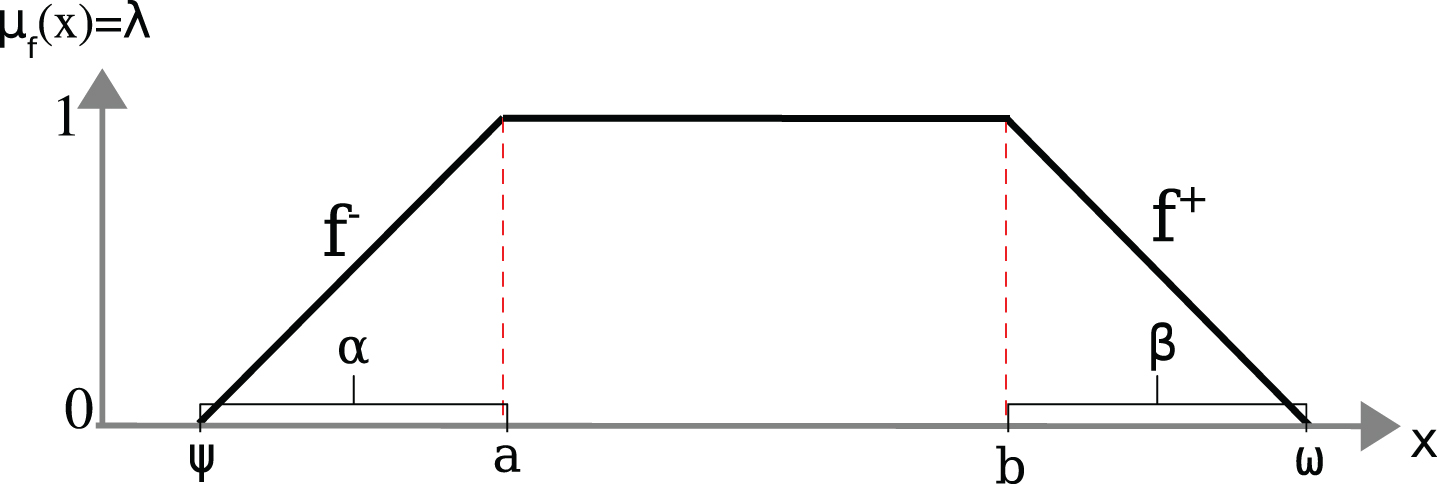
A fuzzy number (if a = b, Fig. 2) defined by [20], is a fuzzy interval. To make their handling more effective, fuzzy intervals are defined using a parametrical representation known as L - R or vertex method [17]. We take two other functions of the form, L (left vertex) and R (right vertex), of $ℝ^{+}$ in [0, 1]. Data can be represented by: an interval with [(a, 1) ; (b, 1) ; α ; β] or two vertex [f^- (left) , f⁺ (right)], a vertex is a function of [0, 1] in $ℝ$ to model the right or left boundary of a fuzzy intervals.

Fig.2

Membership function example.

f⁺ representing the equation of the half-line (b, ω) defined by equation: f⁺ (λ) = - β × λ + (β + b) with β = ω - b [17].

f^- representing the equation of the half-line (ψ, a) defined by equation f^- (λ) = λ × α + (a - α) with α = a - ψ [17].

These two types of representation are shown in Fig. 2.

The data type “Between x and y” is modeled by the interval [a = b = ((x + y)/2, 1) ; ψ = (x, 0) ; ω = (y, 0)].

The data type “Approximately z” is modeled by the interval [a = b = (z, 1) ; ψ = (z - coef, 0) ; ω = (z + coef, 0)] with coef a confidence coefficient.

This mode of representation combines numeric and linguistic representations. To describe a fuzzy interval, and to provide adapted tools to the representation of specialists and their study fields, we offer two methods of construction.

The first method can quickly and simply describe an imprecision. It is based on a description of the interval from reference points, i.e. four couples’ value membership degree, type [(a, 1); (b, 1); (ψ, 0); (ω, 0)]. They are presented in Fig. 2: a and b are the vertex of the membership function; ψ = a - α is the lower limit of the interval; ω = b + β is the upper limit of the interval.

The second method can represent the interval in the equation the form [17, 18]. This style is convenient, simple, intuitive, and can quickly translate an imprecision into graphic form. The use of a visual description is easy to understand and assimilate. Two forms of equations are presented, according to lambda (y-axis, ordinate f^- (λ) = α × λ + (a - α), and f⁺ (λ) = - β × λ + (β + b)) or function of x (x-axis, abscissa $μ^{-} (x) = \frac{x - ψ}{a - ψ}$ and $μ^{+} (x) = \frac{x - ω}{b - ω}$ ). To implement operations on intervals, it may be necessary and appropriate to switch from one to another.

These concepts are included in the fuzzy set theory, with the addition of the membership degree. With the extension principle it was proved that a large part of the operation for classical intervals is usable for fuzzy intervals.

3.1.2 Data handling

The fuzzy intervals are commonly used in approximate reasoning; there has been much research to extend basic operations [17 , 37]. We sort these operations into several categories: standard (+, -, ×, /,...) monotonous functions: function which is either entirely non-increasing or nondecreasing on the interval (sqrt, expo, ln,...), and non-monotonous functions (sin, cos, tan,...). Each of these cases requires the use of specific methods; either the extension principle, the calculation of classical intervals, or the vertex method.

These different methods can perform operations on fuzzy intervals as if they were standard intervals. Depending on the operations, we use the methods that we consider most appropriate and most intuitive. The aim is to promote understanding of operations. For example, the vertex method is used for simple operations (+, -), calculation intervals and the extension principle for more complex operations (×, /, expo, ln, sin, cos, tan,...). Many of these methods and the structure of data are integrated into a class (OOP) to allow the definition and manipulation of the data fuzzy interval type.

In Algorithm 1 we present this class, called FuzzySet. It is possible to create an instance of the class from values a, b, ψ, ω but may have to add a linguistic label characterizing the interval. This linguistic label can make the connection between expert user and mathematical representation.

Algorithm 1
Fuzzy Set class

1: listoperator = $+, -, \times, /, \ln, expo,, \sin, \cos, \tan, . . .$

2: class FuzzySet{

3: intλ ∈ [0, 1] % (figure 2, λ = μ)

4: float a, b, ψ, ω, α = a - ψ, β = ω - b

5: String label

6: functionleft (int λ) = α × λ + (a - α)

7: functionright (int λ) = - β × λ + (β + b)

8: function $left (float x) = \frac{x - ψ}{a - ψ}$

9: function $right (float x) = \frac{x - ω}{b - ω}$

10: % Constructor and functions prototype: out name(in)

11: % Constructor

12: FuzzySet(a, b = a, ψ = a, ω = b, label = ′I′)

13: % Operator with FuzzySet

14: FuzzySetoperator + (FuzzySet)

15: booleanoperator = = (FuzzySet)

16: ...

17: Extension principle function

18: FuzzySetsupMin (FuzzySet, operator)

19: Defuzzification function

20: floatdefuzzification (FuzzySet)

21: ...

22: }

23: % Friends function

24: FuzzySet sin(FuzzySet)

25: FuzzySet tan(FuzzySet)

...

In this class we have implemented various classic operations handling fuzzy intervals and have chosen to use the most appropriate methods to meet our objectives. For instance, for the operation +, we work on the boundary of the interval, from the vertex method. Note that all arithmetic operations or mathematical functions can be performed from the extension principle defined by [47]. In the FuzzySet class, we have developed a generic function that allows us to use this principle, but it is a little slower because it calculates all the values of the interval.

A user who wants to test other methods should redefine our functions. If, for many of the conventional operators, different methods give the same results, a redefinition is not of great interest for other functions, which have been programmed specifically for our needs, their uses can provide results. In this case, it is advisable to adapt to the context.

With this approach a designer has the option in these models to use imprecise variables; to describe the behavior of a system, it is sufficient to use the FuzzySet type.

3.2 iDEVS simulation

The definition of imprecise parameters in models induced simulation problems. If the lifespan of the state is imprecise, it is impossible to define the time of state update. To solve this problem, we have studied several methods.

The first one consists in adapting the simulation algorithms by adding a fuzzy ranking [31, 41]. The goal is to evaluate and sort the different times in terms of execution date, so it is possible to choose which event is triggered. The disadvantage of this solution is that it involves changes to the simulation algorithms which lead us to amend part of the simulation of the DEVS formalism; we set a priority on using the iDEVS approach in any DEVS framework without having to make major changes to the simulation part.

The second solution is the use of a defuzzification function.

Definition: Contrary to the fuzzification, which is the process of transforming crisp values into degree of membership for linguistic terms of fuzzy set, defuzzification is a decision step to transform a fuzzy set into a crisp value.

Based on this definition, we propose to study several solutions. We implemented various defuzzification functions in the FuzzySet class and tested different iDEVS models. The results were the subject of two publications [6, 8]. The function that we believe has the greatest advantages is the Expected Existence Measure (EEM) [1], which allows you to add a decision support. By defining a confidence coefficient, the user can choose when to transform imprecisions on time (if the confidence coefficient is small, between 0 and 0.5, we trigger the event early. The higher the confidence of the coefficient, between 0.5 and 1, the later the event is triggered). In the end we lose information on the x-axis, but we keep the coefficient of the validity of the proposal.

We believe it can be useful, in addition to defuzzifing average validity coefficients, to provide the final result of the interval of time simulation. This interval represents the total time taken by the simulation to be terminated. It is calculated through a state variable type FuzzySet which increments the variable imprecise time (before defuzzification) with each execution of the function.

The method chosen must be included in the DEVS formalism and modify the basic AM to reflect our changes. This step we passed from DEVS to iDEVS because the DEVS AM needs to evolve. This evolution can handle all problems at the level of modeling. It is not necessary to change the simulation algorithms; our starting constraints are met. The problem is linked to time; we modified the time advance function t_a of the AM to return an accurate time, and the defuzzification method was added to the FuzzySet class, Algorithm 1. The algorithm of our new time advance function ${\tilde{t}}_{a}$ is described in Algorithm 2. Thus, the problem of imprecise simulation time is solved by this algorithm. By the addition of this function in the AM, this problem can be handled in the modeling part, so it is not necessary to modify the simulation algorithms. In our case, and given our objectives, the use of a defuzzification function can be seen as a regression. We propose to treat imprecision to ultimately turn it into precise data. The design of the simulator is often done, it is not possible to trigger events at an imprecise time. After studying several methods [1 , 49], this solution seems to be the best one. The use of this function still allows us to take into account imprecision in the other model elements (X,Y,S).

In the AM, time can be defined as imprecise, but it will be defuzzifed before being sent to the simulator. The time advance function was amended to test if the time to return was accurate or imprecise (c.f. Algorithm 2). In the second case, the time is transformed. If the events form a generator model, thus an atomic model, we manage with the time advance function values imprecision on the time of triggering events. Such management requires a fuzzy atomic model to be defined. The difference between the function of the DEVS model and the function of the iDEVS model remains imperceptible to the final user. It is important to note that the first message sent to the simulator, the initialization message, does not contain an imprecise time. Generally, in the DEVS formalism, all events are a source. This is to take into account the case where an event is a source outside the system.

Algorithm 2
time advance function $\tilde{t_{a}}$

% Class variables declaration

FuzzySetτ =new FuzzySet(0, 0, 0, 0, ′tau′) % interval representing the time to end of simulation

float Λ % the sum of membership degrees after defuzzification

floatnbrDefuz ← 1 % variable that counts the number of defuzzificationsfloat $moy Λ = \frac{Λ}{nbrDefuz}$ % variable that keeps the average membership degrees after defuzzification; it is returned at the end of each simulation model

% time advance function

function float $\tilde{t_{a}} ($ stateS) {

  σ the lifespan of the state S

  ifσ is accurate % σ is tested, if σ is accurate the function t_a has a classic behavior

    t_a ← σ

    τ ← τ + σ% intervalτincreases inσ, end simulation will provide an interval time

  else

    t_a ← σ . coefEEM () % σis an instance of the classFuzzySetto which we apply the defuzzification method coefEEM ()[6]

    Λ ← Λ + μ (σ . coefEEM ()) % Λis the sum of defuzzification; functionμ (x) returns an ordinate value for eachx (c.f. figure 2)

    nbrDefuz ← nbrDefuz + 1

    τ ← τ + σ% we add to the intervalτthe intervalσ

  returnt_a

}

In the iDEVS AM, we apply in the time advance function a defuzzification function (EEM), and we keep the degree of validity of the condition (ordinate membership function to the interval: λ) in the form of the coefficient average of the defuzzification lambda. This new variable may be stored as a state system S or added as a class variable in the class atomic model. It is the same for the interval from the time at the end of the simulation. These changes are presented in the next section.

3.3 Models

To take into account the imprecisions in the iDEVS models we must derive or instantiate FuzzySet class. The aim is to provide the designer with ways to define ‘imprecise’ models regardless of the platform or application, just important class in modeling framework. The designer can model a fuzzy system from the combination of iDEVS models derived from the class FuzzySet and a DEVS AM. It is noted that the CM resulting from a combination of ‘imprecise’ models and conventional models is a model that automatically returns imprecise results. All iDEVS models handle imprecision data (data for FuzzySet type), they have the opportunity to use the functions defined in the FuzzySet class.

3.3.1 Atomic model

The iDEVS AM (Fig. 3) is similar to the DEVS AM. Its uniqueness is that it can manipulate variables accurately or imprecisely. Its role is to describe the behavioral aspect of a part of a system with imprecise parameters. If all the parameters of the iDEVS model are accurate, it has the same behavior as a DEVS model.

Fig.3

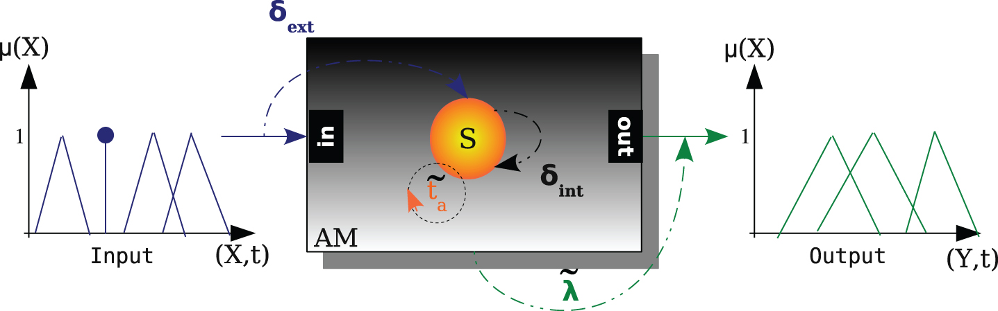
Behavior of an iDEVS atomic model.

In DEVS and iDEVS, the behavior of internal and external transition functions (δ_int, δ_ext) is strictly identical. However, for handling imprecision variables, we use the overloaded functions in FuzzySet (+, -, / cos) class. To describe δ_int and δ_ext, the user need only indicate that the variables are imprecise. The appropriate functions is automatically used. For the time advance functions t_a and output function λ of structural changes were introduced, but they remain imperceptible to the final user. The time advance function of an iDEVS model ${\tilde{t}}_{a}$ must return a crisp value so that the corresponding event can be inserted into the schedule. To this we added a defuzzification function (c.f. Algorithm 2). This function is automatically activated and the final user does not have to worry about its operation. A user can modify the implementation of this function from the FuzzySet class. Another structural change appears in the output function $\tilde{λ}$ . In the end it returns the simulation results, and two class variables that contain the validity degree of the result and the time interval of the simulation.

Generally, the tilde (~) is used to separate fuzzy data from crisp data. In our case, all the parameters of the AM can be imprecise (X, Y, S) or handle imprecise data (t_a, δ, λ). We chose to use the tilde to mark a change from the DEVS model. All parameters of our model could be a tilde, as they may all be imprecise, but only the time advance function ${\tilde{t}}_{a}$ and output function $\tilde{λ}$ were changed. ${AM}_{iDEVS} : < X, Y, S, {\tilde{t}}_{a}, δ_{int}, δ_{ext}, \tilde{λ} >$ (5)

With:

X: is the set of input events characterized by variables: (port, time, value), where time and value can be defined as accurate or imprecise;

Y: is the set of output events, where the value is accurate or imprecise, depending on the behavior of the model;

S: is the set of states or state variables. The state variables can be accurate or imprecise;

$\tilde{t_{a}} : S \to R^{\infty}$ : is the time advance function. Algorithm 2 shows this function;

δ_ext : Q × X → S: is the external transition function which defines how an input event X changes a state of the system, where $Q = {(s, t_{e}) | s \in S, t_{e} \in (T \cap [0, {\tilde{t}}_{a} (s)])}$ is the set of total states, and t_e is the elapsed time since the last event;

$\tilde{λ} : S \to Y^{ι}$ : is the output function where Y^ι = Y ∪ {ι} and ι ∉ Y are a silent event or an unobserved event respectively. This function defines how a state of the system generates an output event, when the elapsed time reaches the lifetime of the state, it returns the model outputs and the class variables τ and moyΛ (Algorithm 2);

δ_int : S → S: is the internal transition function which defines how a state of the system changes internally, when the elapsed time reaches to the lifetime of the state.

The data handled by the iDEVS atomic model are represented by a quadruple [a, b, ψ, ω], defined in the FuzzySet class. If a = b and α = β = 0, the iDEVS model becomes a DEVS model (not fuzzy) handling accurate data. Equation 5 presents in detail the general iDEVS AM.

3.3.2 Coupled model

The iDEVS coupled model has the same form as the DEVS coupled model; both are described in same way. The only difference is that the iDEVS coupled model may consist of a DEVS models or iDEVS models. Therefore the input variables and output are defined as imprecise. Imprecise data includes accurate data.

The iDEVS approach is based on the object-oriented programming concepts. It allows to model and propagate imprecise information with the DEVS formalism. This may be seen as a generalization of the DEVS formalism.

The main advantage of the iDEVS method is the consideration of imprecisions in defining the parameters of the DEVS models in the form of intervals. This description is simple and intuitive, close to the mode of human representation. The limits are: the problem of simulation in imprecise time which requires the use of defuzzification function, and as for the interval arithmetic an increase of the confidence interval after several operations.

After introducing the general forms of iDEVS models in the next section, we present a specific models to describe Fuzzy Inference Systems.

4 Fuzzy Inference Systems with DEVS

The fuzzy inference systems (FIS) are used for reasoning and control as in [44 –46], especially for the simulation of physical or biological systems. They operate from fuzzy reasoning rules, which have the advantage of managing the progressive phenomena.

The design of FIS is based on expert knowledge for the definition of linguistic terms for each input and output variables, and on learning algorithms to generate rules. We present a standard gesture recognition application in [25]. The theoretical and methodological aspects are referenced. The following works [44 –46] provide more extensive vision and applications. We propose to define a new modeling method based on FIS which aims to define a DEVS inference models. The general problem is to consider the best way to put an inference system in DEVS models, to choose the best inference algorithms to use, and to represent the sets of inputs and outputs. As for iDEVS method, a new class FuzzySets was defined; it contains a set of objects of FuzzySet type and different methods for handling as fuzzy sets: conjunction operator MIN, AND, OR.

From this class we can represent the inputs and outputs of the system, and the results obtained following the application of fuzzy operators or inferences methods. We propose accordance with the structure of a fuzzy inference system, to define a model DEVFIS (Discrete Event Fuzzy Inference system Specification [9]) for each stage of the process of inference, namely:

one or more atomic models based on a fuzzification method to represent the input of the system;

one or more atomic models based on a defuzzification method to represent the output of the system;

coupled model describing the inference engine, which includes a atomic model representing all the rules describing the system, atomic model describing the fuzzy operators employees, and an atomic model representing the inference method.

The models are described using the following properties.

4.1 Fuzzy Inference Systems (FIS)

Construction of an FIS consists of several steps: (1) define inputs and outputs vectors, that is to say, match a interval value and a linguistic variable for each input-outputs fuzzy sets. This is the definition of membership functions; (2) determine the rules that describe and reproduce the system behavior; (3) choose the conjunction operators and defuzzification methods. The FIS models used are composed of N rules, which have the following form: $If x_{1} is A_{1}^{i} AND \dot{.} . AND x_{n} is A_{n}^{i} THEN y is B^{i}$ (6) where:

$(x_{i})_{i = 1}^{n}$ are a linguistics variable. A linguistic variable is a variable which takes its values in a set of symbolic “words”; defining the categories of a reference set;

$(A_{j}^{i})_{i = 1}^{N}$ are a fuzzy set defined on the field of linguistic variable x_j, for j = 1 to n;

B are a fuzzy set describing the output field.

The FIS used are either Mamdani type [35], or Takagi-Sugeno type [40]. These are the two forms most commonly used.

These different methods are implemented in the FuzzySets and FuzzySet classes [6], the user has to choose the methods that the wishes.

4.2 FuzzySets class

The FuzzySets class can represent the input and output vectors of the FIS. It is based on a data structure which stores as a list of fuzzy sets. It also provides many methods to manipulate these data. The two methods presented above, and several operators are included in the class.

4.3 FIS DEVS models

A DEVS models used to make the fuzzy inference are classic models.

The input model contains as state variable S the input vector of FIS (fuzzification models Fig. 4), that is to say the fuzzy sets. This is an instance of FuzzySets class, which contains N objects of FuzzySet type. It takes one input and two outputs. When an input is received (crisp value i1 or i2), the external transition function (δ_ext) is triggered, its role is to associate the input value (i1 or i2) to a linguistic label (i1 in A, B, C and i2 in D, E, F - Fig. 4) and to a membership degree (x = i1, μ_B (x) = md1). This information is then transmitted to the following model with the output function λ.

Fig.4

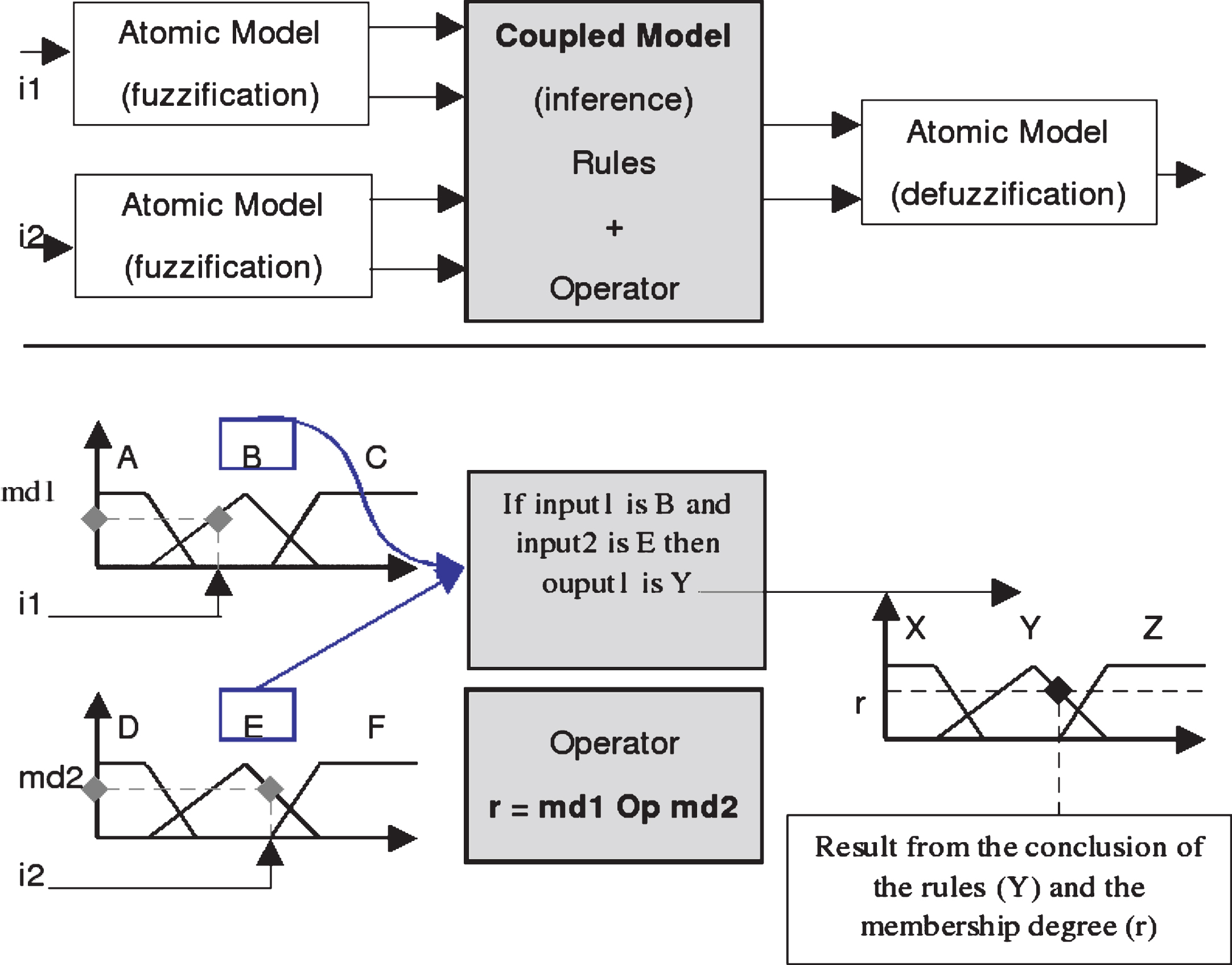
DEVFIS models.

The inference model (Rules + Operator - Fig. 4) is a coupled model composed of two atomic models. It has 2 × N inputs, N being the number of atomic models of fuzzification, and 2 × M outputs, where M is the number of atomic models of defuzzification. The aim of this model is to apply the rules (atomic model rules), and calculate the overall membership degree (atomic model operator).

The first atomic model identifies all the rules in the external transition function (IF i1 == ‘B’ AND i2 == ‘E’, THEN o1 = ‘Y’). Rules’ variables (A, B, C,...) are stored as state variable, or directly in δ_ext. When an input linguistics label is received, δ_ext function is executed. It looks for the conclusion of the rule associated with the linguistics label (if input 1 is A then the conclusion is X). This result is sent with the output function. The methods for making these associations are implemented in the FuzzySets class.

The second model receives the membership degrees (md1 and md2) as input. The δ_ext function calculates, depending on the choice of conjunction operator (AND, OR, MIN, MAX,...), The membership degree of the conclusion of the rule. Its output function returns the calculation result.

The output model (defuzzification model – not used for FIS-type Takagi-Sugeno) has the state variable S, the output vector of FIS (N fuzzy set). This model has two inputs and one output. To receive input data (linguistic label, and overall membership degree, calculated from the conjunction operator), the external transition function is triggered. Its goal is to associate an input data to a crisp value. This value is obtained in two steps: by matching the linguistic label received in input with the linguistic labels of the output fuzzy set, and apply the membership degree, from the inputs, on the ordinate axis of output fuzzy set.

In these models there is no time management, after each input we generate outputs. The models needing more input information are in a temporary state of waiting, as they have received all the necessary data. The method is completely generic, but depending on the application, the models must be redefined. The vectors of inputs, outputs, and rules are specific to the application.

A first application has been made in [4], and we are currently working on the concept of fuzzy activity in cellular automata.

5 Examples

5.1 Fire propagation model example

The example based on cellular automata introduces fuzzification at the level of (propagation rules), we use a fuzzy inference system (FIS) to model fire propagation. It is detailed in [3]. We use it here to illustrate our approach. The simulation API used, along with the class diagram, and the methodology for launching simulations is detailed in [26].

5.1.1 Cellular model

Each cell describes an area of homogeneous vegetation with mass (m) and temperature (T). The behavioural scheme is deterministic and follows five main physical states according to mass and temperature values. (1) Unburnt: the fuel in the cell is at ambient temperature T_a; (2) Heating: the fuel temperature T increases, pyrolysis gases escape, but the fuel never ignites and its mass m remains constant in this state; (3) Burning: the fuel ignites at T_ig and the fuel mass m in the cell decreases; (4) Cooling: the fuel mass m is below the threshold m_ig which maintains the flame, combustion stops (T = T_ext) and the fuel temperature T gradually decreases from Text; (5) Burnt: The fuel mass m is near zero, and the fuel temperature T gradually approaches the ambient temperature T_amb. Figure 5 is an illustration of these cells’ deterministic behavioural profile.

Fig.5

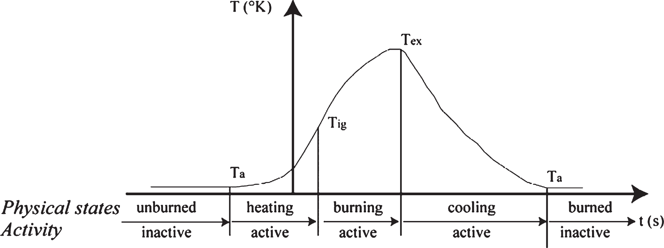
Cell behaviour.

The cell’s is computed from the physical states in the transition function δ, as:

δ_i,j (unburnt, inactive): m₀, T₀;

δ_i,j (heating, active): m_t+1 = m₀, T_t+1 = T₀ + k₁T_t;

δ_i,j (burning, active): m_t+1 = k₃ . (m_t - m_t-1, T_t+1 = T₀ + k₂T_t;

δ_i,j (cooling, active): m_t+1 = m_ext = k₄, T_t+1 = T_ext + k₂T_t;

δ_i,j (burnt, inactive): m_t+1 = m_ext, T_t+1 = T_ext - k₄ . T_t ⇒ T_t+1 ≥ T₀;

where: (i, j) are the cell’s coordinates in the Z_d space, δ the transition function with the physical state as string parameter. The k_i constant is experimentally determined [13, 39]. When a (i, j) cell starts its burning process, it is ‘activated’, until it is burnt. The (i, j) cell becomes ‘inactive’ when its physical state changes to ‘burnt’. Through the simulation process, propagation rules supply the new cells of the fire front, i.e., the cells that have been reached in the neighborhood of active cells at time t+1. Each characteristic time interval corresponds to a couple made of physical state and typical temperature (T_ambient, T_ignition, T_extinction). The active cells of the CAM represent the combustion zone, i.e. the propagation area where the degradation of thermal fuel components occurs. It approximately occurs over a wide range of temperature between 300-900°C. The simulation is focused on active cells according to the discrete time event (DTSS) simulator, in its activity formulation [27 , 36].

5.1.2 Fuzzy model

We use fuzzy logic to explain a doubt in the expression of the propagation rule. Active cells’ behaviour follows a state trajectory which contains partial or temporary states, i.e. possibly active, or PACTIVE. A partial state implies to reevaluate the cell’s activity at the next time step. If there is only one active cell in the neighborhood, the cell remains inactive; if there is more than one active cell in the neighborhood the cell is activated. The activity rules are rewritten to integrate an inference engine and decisional fuzzy rules. The FIS is built according to our works present Sections 2 et 3.

5.1.3 FIS settings

An input fuzzy set is defined with an empirical method, as confirmed by experts, and therefore based on experts experiments and according to the temperature values encountered. Then, the FIS has two Fuzzy Sets: low influence (LOW), and high influence (SUBSTANTIAL) such as the cell temperature in abscissa. The FIS input is the active cell temperature considered. We store the tuple (label, degree of membership) in the neighbouring cells according to the temperature; it is the fuzzification step.

For this neighbouring cells, we get a set of linguistic labels (SUBSTANTIAL ou LOW) of varying sizes. As we do not know before the number of neighbouring cells to influence, i.e. the set size, we use a dynamic inference engine. The fuzzy rules are the following:

if the number of SUBSTANTIAL linguistic labels type is inferior or equal to 1 then the cell is in an INACTIVE state;

if the number of SUBSTANTIAL linguistic labels of type is inferior or equal to 2, then the cell is in a PACTIVE state (Partially Active);

if the number of SUBSTANTIAL linguistic labels of type is higher than 2, then the cell is in an ACTIVE state;

The output fuzzy set describes activity level according to the number of neighboring cells and fuzzy rules.

Thanks to the inference engine, we obtain an activity value. After the defuzzification process, we obtain the activity level for each active cell.

5.1.4 Results

Figure 6 is an illustration of simulation rendering by means of fuzzy rules. A conventional fire propagation is well represented.

Fig.6

Fire spreading evolution with fuzzy rules.

Figure 7 illustrates different FIS setups, and shows that few modifications FIS parameters can have high impact on propagation behaviour, consequently, the results should be very different in terms of rendering. The results obtained underline the importance of implementing fuzzy activity in a CAM. The interest of this approach is to define a propagation rule from simple linguistic rules expressed in natural language.

Fig.7

Six different FIS setup rendering.

This example shows the adaptation of the method. We use here a specific simulator adapted to the discrete time system (DTSS). This DTSS formalism is a special case of the DEVS formalism.

5.2 Other case studies

Our approach has been already applied in several application fields:

to solve a first order imprecise equation to study the mechanical part of the induction machine [5];

to compare defuzzification methods for discrete event systems [7];

to define a predictive wind model with imprecise parameters to select the location of wind turbines [6];

to design a decision-making model controlling the boiler temperature and stream-flow [4];

to study forest fire spreading [3 , 12];

to take into account the knowledge evolution over time [2].

to model the lack of knowledge in the propagation rules of a cellular automaton [3].

The interested reader may refer to the mentioned papers. Details on methodology and applications are presented. For us, these case studies provide several proofs of concept that demonstrate the usability and the genericity of our approach.

6 Conclusion

In this article, we have presented a synthesis of several conference papers. The aim of our work is to bridge the Theory of Modeling and Simulation (TMS), through the DEVS formalism, and the Fuzzy Set Theory. The approach presented is based on mathematical definitions of the Fuzzy Set Theory to represent and use imprecise information in the DEVS formalism. A methodology based on the notions of object oriented programming is proposed: to describe imprecision in the form of data structures and manipulate them as classical objects (int, float...); to generalize the DEVS formalism, and thus allow to model and propagate imprecise information. It is called iDEVS: to take into account imprecision in the DEVS formalism. The aim is to allow users of the DEVS formalism to describe systems with imprecise parameters, and to propagate this imprecision by simulation. Finally, an analogy is proposed between Fuzzy Interference Systems and iDEVS models. In this analogy we have proposed to facilitate controller modeling and to open the application domains of the DEVS formalism to all fields of application of fuzzy interference systems (FIS). The method is generic and allows to represent and use FIS in DEVS. This makes it possible to open the DEVS formalism to other domains (decision support), and to bring together the tools based on the DEVS formalism of commercial tools that offers fuzzy toolbox. The approach is still limited in number of defuzzification function for example, and it also lacks a graphical interface for the design of the rules of the interference engine. Currently it is necessary to do it in the code, it is not very user friendly.

As for the interval arithmetic, the main limitation of this approach is that the more the simulation time advances more the confidence interval increases. This problem requires the use of defuzzification functions to limit combinatorial explosions.

At the perspective level, an interesting work to show the advantage of our approach would be to make comparisons with other tools. The approach must be improved, in particular to complete the mathematical functions to handle fuzzy sets. We are also interested in fuzzy ranking methods for managing the DEVS formalism scheduled. We are currently working on using our approach as a decision model for autonomous agents, more recently, we are thinking about using fuzzy logic as a tool to improve confidence in simulation results.

Footnotes

Acknowledgments

The authors would like to thank the Corsican Region (CTC) and the European Union (EU) to support MoonFish po-feder project.

References

Anglani

, Grieco

, Nucci

, Semeraro

and Tolio

, A sound analysis of fuzzy simulation results., In Proceedings of Intelligent Computation in Manufacturing Engineering 2000 citeseer.ist.psu.edu/496399.html. Capri, Naples, Italy (2000).

Bisgambiglia

, Bisgambiglia

P.A.

and Gualtieri

, Cognitive simulation-based on knowledge evolution in fuzzy discrete event systems., In Fuzzy Systems (FUZZ), 2011 IEEE International Conference on Fuzzy Systems (FUZZ-IEEE 2011) pp. 895–901. IEEE

Bisgambiglia

, Innocenti

and Gonsolin

, A new way to use Fuzzy Inference Systems in Activity-Based Cellular Modeling Simulations., In International Conference on Fuzzy Systems (FUZZ-IEEE 2017) (2017), IEEE.

Bisgambiglia

P.-A.

, Capocchi

, Bisgambiglia

and Garredu

, Fuzzy Inference Models For Discrete EVent Systems., In Proceedings of the 2010 IEEE World Congress on Computational Intelligence (WCCI 2010) - IEEE International Conference on Fuzzy Systems (FUZZ-IEEE) (2010), pp688–694.

Bisgambiglia

P.-A.

, Capocchi

and de Gentili

, Bisgambiglia

, Manipulation of incomplete or fuzzy Data for DEVS-based Systems., In SCS, editor, In Proceedings of the International Modeling and Simulation Multiconference (IMSM) - Conceptual Modeling Simulation (CMS) (2007), pp. 87–92.

Bisgambiglia

P.-A.

and de Gentili

, Bisgambiglia

and Santucci

, Discrete Events System Simulation-based de-Fuzzification method. In Proceedings of The 14th IEEE Mediterranean Electrotechnical Conference (MELECON) (2008a), pp. 132–138.

Bisgambiglia

P.-A.

and de Gentili

, Bisgambiglia

and Santucci

, Fuzzy Modeling for Discrete Events Systems. In Proceedings of The 14th IEEE Mediterranean Electrotechnical Conference (MELECON) (2008b), pp. 151–157.

Bisgambiglia

P.-A.

and de Gentili

, Bisgambiglia

and Santucci

, Fuzzy Simulation for Discrete Events Systems., In Proceedings of the 2008 IEEE World Congress on Computational Intelligence (WCCI 2008) - IEEE International Conference on Fuzzy Systems (FUZZ-IEEE) (2008c), pp. 688–694.

Bisgambiglia

P.-A.

and de Gentili

, Bisgambiglia

and Santucci

J.-F.

, Fuzz-iDEVS: Towards a fuzzy toolbox for discrete event systems., In ACM, editor, Proceedings of the SIMUTools’ 09, Rome (Italie) (2009a), SIMUTools.

10.

Bisgambiglia

P.-A.

and de Gentili

, Bisgambiglia

and Santucci

J.-F.

, iDEVS: New method to study inaccurate systems., In IEEE, editor Proceedings of the The Annual IEEE International Conference on Fuzzy Systems, Jeju Island, Korea, (2009b), IEEE.

11.

Bisgambiglia

P.-A.

and de Gentili

, Santucci

and Bisgambiglia

, DEVS-Flou: A Discrete Events and Fuzzy Sets Theory-Based Modeling Environment., In IEEE, editor, Proceedings of the Systems and Control in Aerospace and Astronautics, (ISSCAA) (2006a), pp. 95–100.

12.

Bisgambiglia

P.-A.

, Filippi

and de Gentili

, A fuzzy approach of modeling evolutionary interfaces systems., In IEEE, editor,Proceedings of the ISEIM 2006, Corte (France) (2006b), pp. 98–103.

13.

Cancellieri

, Innocenti

and Leroy-Cancellieri

, Wingpyro: A software platform for kinetic study of forest fuels, Fire Safety Journal 58 (2013), 103–111.

14.

Cassandrass

and Lafortune

, Introduction to Discrete Event Systems Boston, Kluwer Academic Publishers, 1999

15.

, Ying

and Lin

, Theory of extended fuzzy discrete-event systems for handling ranges of knowledge uncertainties and subjectivity, IEEE Transactions on Fuzzy Systems 17(2) (2009), 316–328.

16.

, Ying

and Lin

, On modeling of fuzzy hybrid systems, Journal of Intelligent & Fuzzy Systems 23(4) (2012), 129–141.

17.

Dubois

, Fargier

and Fortin

, A generalized vertex method for computing with fuzzy intervals., In IEEE, editor, Proc of the International Conference on Fuzzy Systems IEEE. Budapest, Hungary, (2004), pp. 541–546.

18.

Dubois

, Fargier

and Fortin

, The empirical variance of a set of fuzzy intervals, IEEE (2005).

19.

Dubois

and Prade

, Fuzzy sets and systems Academic Press, 1980.

20.

Dubois

and Prade

, Fuzzy set in approximate reasoning, part 1, Fuzzy set and Systems 40 (1993).

21.

Fortin

, Zielinski

, Dubois

and Fargier

, Interval analysis in scheduling., In van Beek

, editor, Proc of the 11th International Conference on Principles and Pratice of Constraint Programming (CP’05) Sitges Spain, Springer, (2005), pp. 226–240.

22.

Giambasi

, Escude

and Ghosh

, GDEVS: A Generalized Discrete Event Specification for Accurate Modeling of Dynamic Systems, Transactions of the Society for Computer Simulation International (2000), pp. 120–134.

23.

Giambiasi

and Ghosh

, Min-Max-DEVS: A new formalism for the specification of discrete event models with minmax delays,, In Proceedings of 13th European Simulation Symposium (2001), pp. 616–621.

24.

Grieco

, Nucci

and Anglani

, Representation of fuzzy time variables in discrete event simulation, Integrated Computer-Aided Engineering 4(4) (2003), 305–318.

25.

Gualtieri

J.-S.

and Bisgambiglia

P.-A.

, A polyphony learning software (pls) based on gesture recognition by fuzzy inference system, Journal of Intelligent & Fuzzy Systems 28(4) (2015), 1795–1803.

26.

Innocenti

, Bisgambiglia

P.-A.

and Urbani

, Activity-based discrete event simulation of spatial production systems: Application to fisheries, In Advances in Production Management Systems. Innovative and Knowledge-Based Production Management in a Global-Local World Springer, (2014), pp.240–247.

27.

Innocenti

and Cancellieri

, Randomizing activity in fire spreading simulations, In ITM Web of Conferences volume 1, EDP Sciences 2013.

28.

Innocenti

, Muzy

, Hill

, Aiello

and Santucci

J.-F.

, Design of a multithreaded parallel model for fire spread, In 15 th European Simulation Symposium (2003), pp. 104–10.

29.

Kilic

, Karasu

and Leblebicioglu

, Fault diagnosis with dynamic fuzzy discrete event system approach, Transactions in Artificial intelligence and neural networks (14th Turkish Symposium, TAINN 2005, Izmir, Turkey, June 16-17, 2005) (revised selected papers) (2005), pp. 117–124.

30.

Kwon

, Park

, Jung

and Kim

, Fuzzy-DEVS Formalisme: Concepts, Realization and Application., Proceedings AIS 1996 (1996), pp. 227–234.

31.

Lee

, Lee

K.H.

and Lee

, Ranking the sequences of fuzzy values, Inf Sci Inf Comput Sci 160(1-4) (2004), 41–52.

32.

Lin

and Ying

, Fuzzy discrete event systems and their observability, In IEEE, editor, Proceedigns of IFSA World Congress and 20th NAFIPS International Conference Vancouver, Canada, volume 3, (2001), pp. 1271–1276.

33.

Lin

and Ying

, Modeling and control of fuzzy discrete event systems, IEEE Transactions on Systems, Man, and Cybernetics, Part B: Cybernetics 32(4) (2002), 408–415.

34.

Lin

, Ying

, MacArthur

R.D.

, Cohn

J.A.

, Barth-Jones

and Crane

L.R.

, Decision making in fuzzy discrete event systems, Inf Sci 177 (2007), 3749–3763.

35.

Mamdani

, Advances in the linguistic synthesis of fuzzy controllers, International Journal of Man-Machine Studies 8(6) (1976), 669–678.

36.

Mathey

A.-H.

, Krcmar

, Dragicevic

and Vertinsky

, An object-oriented cellular automata model for forest planning problems, Ecological Modelling 212(3) (2008), 359–371.

37.

Moore

, Interval Analysis, 1966.

38.

Qiu

and Liu

, Fuzzy Discrete Event Systems under Fuzzy Observability and a test-algorithm, ArXiv Computer Science e-prints 2006.

39.

Santoni

P.-A.

, Balbi

J.-H.

, Bosseur

, Innocenti

, Marcelli

, Morandini

, Nasica

, Pieri

, Rinieri

and Rossi

J.-L.

et al., Metrology of windland fire: Characterization of a fire spreading across the corsican scrub, congrés Environnement et Identité en Méditerranée, Université de Corse, (2004), pp. 1–8.

40.

Takagi

and Sugeno

, Fuzzy indentification of systems and its applications to modeling and control, In IEEE, editor, Proceedings in IEEE Trans On S.M.C 1985.

41.

Tran

and Duckstein

, Comparison of fuzzy numbers using a fuzzy distance measure, Fuzzy Sets Syst 130(3) (2002), 331–341.

42.

Vangheluwe

, DEVS as a Common Denominator for Multi-Formalism Hybrid Systems Modelling., In Proceedings of ISCACS 2000 2000.

43.

Vangheluwe

, The Discrete EVent System specification DEVS Formalism, Technical report, http://moncs.cs.mcgill.ca/, (2001).

44.

Wei

, Qiu

and Karimi

H.R.

, Reliable output feedback control of discrete-time fuzzy affine systems with actuator faults, IEEE Transactions on Circuits and Systems I: Regular Papers 64(1) (2017a), 170–181.

45.

Wei

, Qiu

and Lam

H.-K.

, A novel approach to reliable output feedback control of fuzzy-affine systems with time-delays and sensor faults, IEEE Transactions on Fuzzy Systems (2016).

46.

Wei

, Qiu

, Lam

H.-K.

and Wu

, Approaches to t– s fuzzy-affine-model-based reliable output feedback control for nonlinear ito stochastic systems, IEEE Transactions on Fuzzy Systems 25(3) (2017b), 569–583.

47.

Zadeh

, Fuzzy sets, Information Control 8 (1965), 338–353.

48.

Zeigler

B.P.

, Praehofer

and Kim

T.G.

, Theory of Modeling and Simulation, Second Edition, Inc, Academic Press, 2000.

49.

Zhang

, Tam

M.C.

and Li

, Modeling uncertain activity duration by fuzzy number and discrete-event simulation, European Journal of Operational Research 164(3) (2005), 573–695.