Optimizing portfolio selection problems under credibilistic CVaR criterion

Abstract

Portfolio optimization is concerned with the optimal allocation of limited capital to the available financial assets to achieve a reasonable tradeoff between risk and profit. The main contribution of this paper is to introduce a new risk measure, conditional value-at-risk (CVaR) of fuzzy variable, to build a class of credibilistic mean-CVaR portfolio optimization model. In the proposed credibilistic portfolio optimization model, the CVaR is used as a measure tool to assess market risk resulted from the financial asset price fluctuations. The computational formulas for common triangular, trapezoidal and normal fuzzy variables are established. Under mild assumptions on the uncertain returns, the proposed credibilistic portfolio optimization model can be turned into its equivalent deterministic mixed-integer parametric programming models, which can be solved by the CPLEX software. The computational results from our numerical experiments demonstrate the efficiency of the proposed CVaR modeling approach as a risk management tool.

Keywords

Portfolio optimization risk management financial asset conditional value-at-risk credibilistic optimization

1 Introduction

Risk management has received much attention in portfolio selection problems, with variance emerging as one of popular tools [28]. The classical mean-variance model [39] formulated the portfolio selection problem as a bi-criteria optimization problem with a tradeoff between risk and profit. The developments of stochastic portfolio optimization are motivated by the following two basic requirements, one is to model adequately the utility functions, risks and constraints [17], another is to address the computational efficiency for handling large numbers of scenarios [30, 57]. In addition, the technique of stochastic dynamic programming has been applied to multi-period portfolio selection problems [2 , 49].

In the literature, variance as a risk measure has been widely criticized by practitioners due to its symmetrical measure with equally weights desirable positive returns and undesirable negative returns [23]. This limitation has led to the research directions where realistic risk measures are used to separate undesirable downside movements from desirable upside movements. Among those risk measures, Vale-at-Risk (VaR) and expected shortfall are the widely accepted popular risk measures [20 , 46, 53]. Furthermore, when the distribution information of stochastic returns are partially available, robust portfolio optimization problems have also been studied in the literature [22, 24]. Robust optimization was also used to tackle effectively a newsvendor problem [55].

Since the concept of fuzzy set was introduced in the seminal work of Zadeh [58], fuzzy theory and its applications have been well-developed by a number of researchers [5–10 , 59]. The developed fuzzy techniques have been used to model portfolio selection problems [4 , 60], in which the variance of fuzzy variable was used as a risk management tool on an agent’s portfolio selection problem. As for various extensions of the fuzzy mean-variance model, the interested reader may further refer to [32 , 54].

In fuzzy decision systems, the downside risk measures like absolute semi-deviation and value-at-risk of fuzzy variables have also been studied [1 , 51]. Among them, Chen et al. [12] introduced the absolute semi-deviation of fuzzy variable by nonlinear fuzzy integrals, and developed three classes of mean-absolute-semideviation fuzzy portfolio optimization models. Based on the VaR optimization criterion, Liu and Liu [35] discussed how uncertainty and interaction impact the project portfolio return and staff allocation. Wang et al. [51] proposed a VaR-based fuzzy portfolio selection model, where the VaR can directly reflect the greatest loss of a selected portfolio under a given confidence level.

The motivation of this paper is based on the following considerations. Among the downside risk measures in fuzzy portfolio optimization problems, there is no study about the CVaR of fuzzy variable. The difficulty to define such a risk measure is that there is no conditional expectation of fuzzy variable we can apply in fuzzy decision systems. To overcome this difficulty, this paper addresses an alternative approach to defining the CVaR risk measure. Our approach is based on a desirable property that the VaR is an optimal solution to an unconstrained optimization problem. The proposed CVaR can measure adequately the tail information of the loss distribution. That is, for the loss of the portfolio that exceeds a given VaR, the CVaR can effectively measure its risk information.

Overall, this paper contributes to the area of portfolio optimization and management in the following three aspects:

First, it introduces a new concept about the CVaR of fuzzy variable. The proposed CVaR is the optimal objective value of a convex optimization model with the VaR being its optimal solution, and is a new downside risk measure that can measure the tail risk adequately.

Second, our proposed optimization approach employs the CVaR risk measure to separate undesirable downside movements from desirable upside movements, thus it is an enhancement of the traditional mean-variance portfolio optimization.

Third, when fuzzy returns follow common credibility distributions, the equivalent deterministic parametric programming models of the proposed mean-CVaR model are computationally tractable due to their linear objective and constraint functions. Hence, from the computational viewpoint, the proposed mean-CVaR model has some advantages over the traditional mean-variance approach.

The rest of the paper is structured as follows. Section 2 introduces the concept CVaR of fuzzy variable and establishes the CVaR computational formulas for common credibility distributions. Section 3 formulates the mean-CVaR model and derives its equivalent deterministic mixed-integer programming models. Section 4 discusses the performance of the proposed mean-CVaR modeling approach and compares this method with the existing mean-risk optimization method. Finally, conclusions and future work are presented in Section 5. All proofs are given in the Appendix.

2 The CVaR risk measure

In credibilistic optimization models, one way for addressing simultaneously the loss size and the credibility of loss requires the fractiles of fuzzy variable. If ξ is a fuzzy variable with monotone increasing credibility function F_ξ (r) = Cr {ξ ≤ r} and 0 < α < 1, then $r \in R$ is called an α-fractile provided that the following two inequalities $Cr {ξ \leq r} \geq α and Cr {ξ \geq r} \geq 1 - α$ hold true, where Cr is the credibility measure defined in [33].

Assume that 0 < α < 1 holds and define the following Value-at-Risk (VaR) for fuzzy variable ξ: $ρ_{VaR}^{α} (ξ) = min {r ∣ F_{ξ} (r) \geq α} .$ (1)

According to this definition, for a given credibility level α, $ρ_{VaR}^{α} (ξ)$ is the left endpoint of the closed interval of α-fractiles of ξ, and sometimes denoted as v_α.

Based on the expected value of fuzzy variable [33], one has the following convexity property about unconstrained optimization problem (2):

Theorem 1. Let ξ be a fuzzy variable with finite expected value and the credibility level 0 < α < 1. Then the following unconstrained optimization problem $min_{z} [z + \frac{1}{1 - α} E [(ξ - z)^{+}]]$ (2) is a convex programming in variable z, where (a) ⁺ = max {a, 0}.

Under the assumption that F_ξ (r) = Cr {ξ ≤ r} is continuous, the set of solutions to problem (2) consists of the set of α-fractiles of fuzzy variable ξ. Indeed, by the following integral representation $u (z) = z + \frac{1}{1 - α} \int_{z}^{\infty} (1 - F_{ξ} (r)) d r,$ the function u (z) is continuously differentiable. Since problem (2) is a convex programming, the set of optimal solutions is determined by the following equation $\frac{d u (z)}{d z} = 0,$ which is written as $1 - \frac{1}{1 - α} (1 - F_{ξ} (z)) = 0 \Leftrightarrow F_{ξ} (z) = α,$ which implies the solution set of problem (2) is the set of α-fractiles of ξ.

The above analysis motivates us to introduce the following new risk measure for fuzzy variables:

Definition 1. Let ξ be a fuzzy variable with finite expected value and the credibility level 0 < α < 1. Then the α-CVaR of fuzzy variable ξ is defined as $ρ_{CVaR}^{α} (ξ) = min_{z} [z + \frac{1}{1 - α} E [(ξ - z)^{+}]],$ (3) where (ξ - z) ⁺ = max {ξ - z, 0}.

The CVaR risk measure is defined on the linear space of fuzzy variables with finite expected values. If F_ξ (r) is continuous, then VaR v_α is an optimal solution to problem (2). As a result, the following inequality holds true: $ρ_{CVaR}^{α} (ξ) \geq ρ_{VaR}^{α} (ξ)$ for any prescribed credibility level 0 < α < 1.

For a fuzzy variable with a triangular credibility distribution [21], its α-CVaR computational formula is given in the following theorem:

Theorem 2. If ξ ∼ Tri (r₁, r₂, r₃) is a triangular fuzzy variable and the credibility level 0 < α < 1, then its α-CVaR is computed by $\begin{matrix} ρ_{CVaR}^{α} (ξ) \\ = {\begin{matrix} \frac{(1 - 2 α)^{2} r_{1}}{4 (1 - α)} + \frac{(1 - 2 α^{2}) r_{2}}{2 (1 - α)} + \frac{r_{3}}{4 (1 - α)}, & 0 < α \leq 0.5 \\ (1 - α) r_{2} + α r_{3}, & 0.5 < α < 1 . \end{matrix} \end{matrix}$

The next theorem discusses the α-CVaR computational formula for a trapezoidal fuzzy variable:

Theorem 3. If ξ ∼ Tra (r₁, r₂, r₃, r₄) is a trapezoidal fuzzy variable and the credibility level 0 < α < 1, then its α-CVaR is computed by $\begin{matrix} ρ_{CVaR}^{α} (ξ) \\ = {\begin{matrix} \frac{(1 - 2 α)^{2} r_{1}}{4 (1 - α)} + \frac{(1 + 2 α) (1 - 2 α) r_{2}}{4 (1 - α)} + \frac{r_{3}}{4 (1 - α)} + \frac{r_{4}}{4 (1 - α)}, \\ 0 < α \leq 0.5 \\ (1 - α) r_{3} + α r_{4}, 0.5 < α < 1 . \end{matrix} \end{matrix}$

The following theorem deals with the α-CVaR computational formula for a normal fuzzy variable:

Theorem 4. If ξ ∼ n (m, σ²) is a normal fuzzy variable and the credibility level 0 < α < 1, then its α-CVaR is computed by $\begin{matrix} ρ_{CVaR}^{α} (ξ) \\ = {\begin{matrix} m + (- \sqrt{2 ln (1 / 2 α)} + \frac{\sqrt{2 ln (1 / 2 α)}}{1 - α} \\ + \frac{\sqrt{2 π} Φ (- \sqrt{2 ln (1 / 2 α)})}{2 (1 - α)}) σ, 0 < α \leq 0.5 \\ m + (\sqrt{2 ln (1 / 2 (1 - α))} \\ + \frac{\sqrt{2 π} (1 - Φ (\sqrt{2 ln (1 / 2 (1 - α))}))}{2 (1 - α)}) σ, 0.5 < α < 1, \end{matrix} \end{matrix}$ where $Φ (t) = \frac{1}{\sqrt{2 π}} \int_{- \infty}^{t} exp (- s^{2} / 2) d s$ .

Taking the CVaR as a risk measure, a new class of credibilistic mean-CVaR portfolio optimization model will be built in the next section.

3 Fuzzy portfolio optimization model under CVaR criterion

3.1 Formulation of mean-CVaR model

A portfolio manager may use his/her experience in stock picking to decide on an appropriate mix of assets in the portfolio selection process. For illustrating the use of the proposed CVaR risk measure in practice, we present a novel credibilistic portfolio selection model. We consider a one-period financial portfolio optimization problem with n risk assets. Denote η^T = (η₁, η₂, …, η_n) as the vector of fuzzy returns of assets and r_i = E [η_i], i = 1, 2, …, n, the mean returns, where the fuzzy vector η is assumed to follow a known joint credibility distribution.

A portfolio is a collection of nonnegative numbers x_j, j = 1, 2, …, n, that sum to one. The return one would obtain using a given portfolio is given by η^Tx. Since for the CVaR risk measure we have interpreted negative values of fuzzy returns as losses, we take ζ (x, η) = - η^Tx. Thus, the expected value E [η^Tx] of η^Tx and CVaR $ρ_{CVaR}^{α} (ζ (x, η))$ of ζ (x, η) are taken as the investment mean return and risk, respectively. If we use μ_p to stand for a prescribed minimum mean portfolio return level, then the mean return E [η^Tx] of a portfolio x = (x₁, x₂, …, x_n) should satisfy the following constraint $E [η^{T} x] \geq μ_{p} .$ (4)

If y_j is a binary variable that is equal to 1 if asset j is selected in the portfolio and 0 otherwise, then $\sum_{j = 1}^{n} y_{j}$ is the number of assets selected to invest in. If m is assumed to be the maximum number of assets that can be selected in the portfolio, then the following constraints should hold true: $\sum_{j = 1}^{n} y_{j} \leq m, y_{j} = 0 or 1, j = 1, 2, \dots, n .$ (5)

Since the investment proportions will not be infinitesimal in actual investment operations, we introduce the lower bound l_j of fraction of the capital budget that can be invested in the jth asset. Taking into account the issue of investment diversification, we also introduce the upper bound u_j of the fraction. These considerations can be represented as $l_{j} y_{j} \leq x_{j} \leq u_{j} y_{j}, j = 1, 2, \dots, n .$ (6)

In addition, a portfolio should satisfy the following constraints under the assumption that short sales are not permitted: $\sum_{j = 1}^{n} x_{j} = 1, x_{j} \geq 0, j = 1, 2, \dots, n .$ (7)

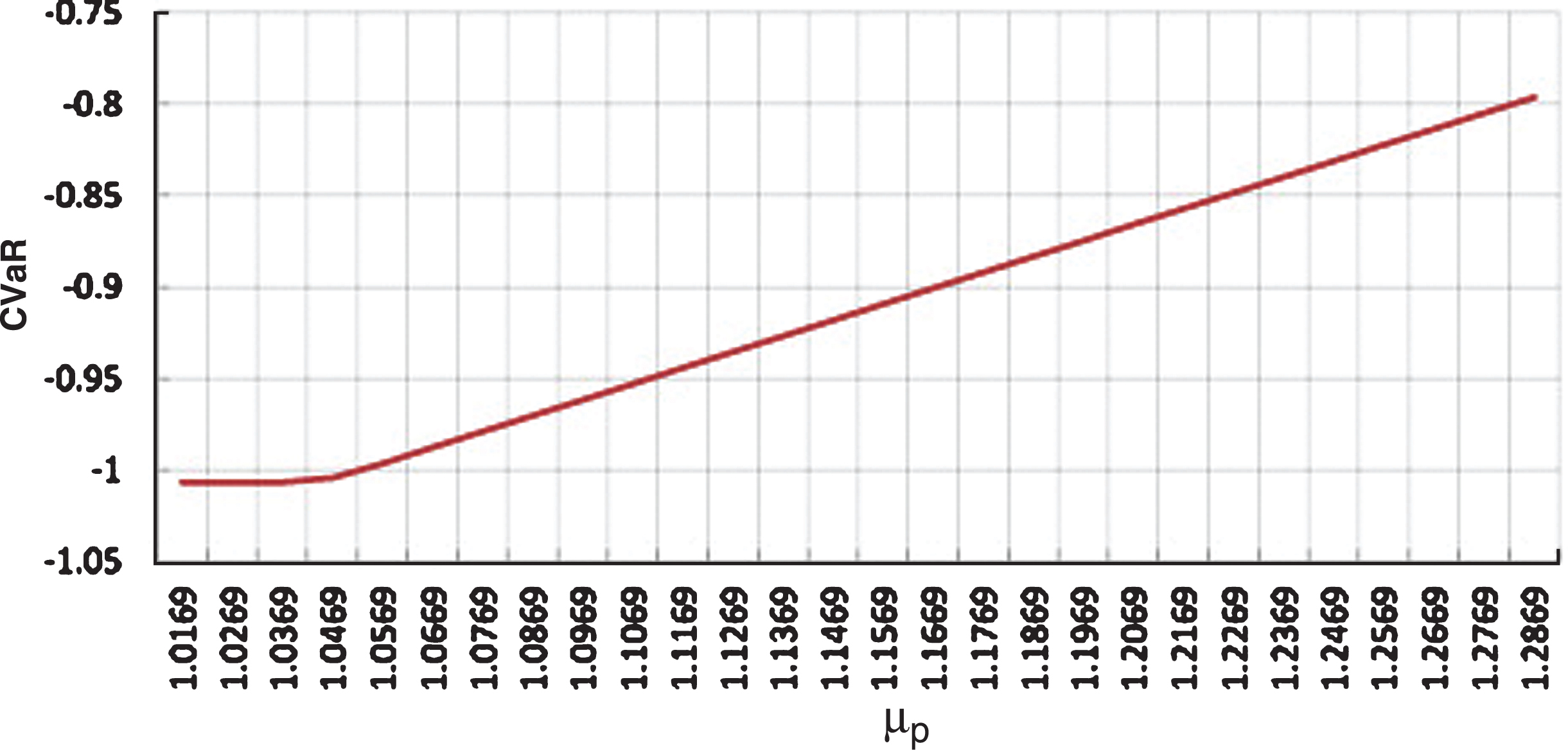
As a consequence, to find a portfolio with the minimum risk, we develop a new credibilistic mean-CVaR optimization model in the following form: ${\begin{matrix} Ψ (μ_{p}) = min & ρ_{CVaR}^{α} (ζ (x, η)) \\ s . t . & constraints (4) - (7) . \end{matrix}$ (8)

The interpretation of mean-CVaR model (8) is as follows: the portfolio manager is looking for a portfolio with the minimum risk in the sense of CVaR, under prescribing a minimum acceptable level μ_p of mean portfolio return.

In mean-CVaR model (8), the optimal objective value Ψ (μ_p), as a function of μ_p, plays an important role. The graph of Ψ (μ_p) in $R^{2}$ is called the efficient frontier, which is usually represented graphically with the horizontal axis corresponding to risk in the sense of CVaR and the vertical axis corresponding to return.

3.2 Analysis of the mean-CVaR model

To solve mean-CVaR model (8), we now identify the cases when model (8) can be turned into its equivalent deterministic programming model. Under the assumptions that fuzzy returns are mutually independent in the sense of [36], and follow common credibility distributions [21], one can obtain the desirable results, which are provided in the following theorems.

Firstly, when fuzzy returns follow the triangular credibility distributions, one has the following results:

Theorem 5. Suppose η_i ∼ Tri (r_i1, r_i2, r_i3), i = 1, 2, …, n, are mutually independent fuzzy returns with triangular credibility distributions.

If the credibility level 0 < α ≤ 0.5, then mean-CVaR model (8) is equivalent to the following mixed-integer parametric programming ${\begin{matrix} min - \sum_{i = 1}^{n} [\frac{(1 - 2 α)^{2} r_{i 3}}{4 (1 - α)} + \frac{(1 - 2 α^{2}) r_{i 2}}{2 (1 - α)} \\ + \frac{r_{i 1}}{4 (1 - α)}] x_{i} \\ s . t . \frac{1}{4} \sum_{i = 1}^{n} [r_{i 1} + 2 r_{i 2} + r_{i 3}] x_{i} \geq μ_{p} \\ (5) - (7) . \end{matrix}$ (9)

If the credibility level 0.5 < α < 1, then mean-CVaR model (8) is equivalent to the following mixed-integer parametric programming ${\begin{matrix} min - \sum_{i = 1}^{n} [(1 - α) r_{i 2} + α r_{i 1}] x_{i} \\ s . t . \frac{1}{4} \sum_{i = 1}^{n} [r_{i 1} + 2 r_{i 2} + r_{i 3}] x_{i} \geq μ_{p} \\ (5) - (7) . \end{matrix}$ (10)

Secondly, when fuzzy returns follow the trapezoidal credibility distributions, one has the following results:

Theorem 6. Suppose η_i ∼ Tra (r_i1, r_i2, r_i3, r_i4), i = 1, 2, …, n, are mutually independent fuzzy returns with trapezoidal credibility distributions.

If the credibility level 0 < α ≤ 0.5, then mean-CVaR model (8) is equivalent to the following mixed-integer parametric programming ${\begin{matrix} min - \sum_{i = 1}^{n} [\frac{(1 - 2 α)^{2} r_{i 4}}{4 (1 - α)} + \frac{(1 - 4 α^{2}) r_{i 3}}{4 (1 - α)} \\ + \frac{r_{i 2}}{4 (1 - α)} + \frac{r_{i 1}}{4 (1 - α)}] x_{i} \\ s . t . \frac{1}{4} \sum_{i = 1}^{n} [r_{i 1} + r_{i 2} + r_{i 3} + r_{i 4}] x_{i} \\ \geq μ_{p}, (5) - (7) . \end{matrix}$ (11)

If the credibility level 0.5 < α < 1, then mean-CVaR model (8) is equivalent to the following mixed-integer parametric programming ${\begin{matrix} min - \sum_{i = 1}^{n} [(1 - α) r_{i 2} + α r_{i 1}] x_{i} \\ s . t . \frac{1}{4} \sum_{i = 1}^{n} [r_{i 1} + r_{i 2} + r_{i 3} + r_{i 4}] x_{i} \\ \geq μ_{p}, (5) - (7) . \end{matrix}$ (12)

Finally, when fuzzy returns follow the normal credibility distributions, one has the following results:

Theorem 7. Suppose $η_{i} \sim n (m_{i}, σ_{i}^{2})$ , i = 1, 2, …, n, are mutually independent fuzzy returns with normal credibility distributions.

If the credibility level 0 < α ≤ 0.5, then mean-CVaR model (8) is equivalent to the following mixed-integer parametric programming ${\begin{matrix} min \sum_{i = 1}^{n} [- m_{i} + (- \sqrt{2 ln (1 / 2 α)} \\ + \frac{\sqrt{2 ln (1 / 2 α)}}{1 - α} + \frac{\sqrt{2 π} Φ (- \sqrt{2 ln (1 / 2 α)})}{2 (1 - α)}) σ_{i}] x_{i} \\ s . t . \sum_{i = 1}^{n} m_{i} x_{i} \geq μ_{p}, (5) - (7) . \end{matrix}$ (13)

If the credibility level 0.5 < α < 1, then mean-CVaR model (8) is equivalent to the following mixed-integer parametric programming ${\begin{matrix} min \sum_{i = 1}^{n} [- m_{i} + (\sqrt{2 ln (1 / 2 (1 - α))} \\ + \frac{\sqrt{2 π} (1 - Φ (\sqrt{2 ln (1 / 2 (1 - α))}))}{2 (1 - α)}) σ_{i}] x_{i} \\ s . t . \sum_{i = 1}^{n} m_{i} x_{i} \geq μ_{p}, (5) - (7) . \end{matrix}$ (14)

On the basis of Theorems 5, 6 and 7, when fuzzy returns are mutually independent and follow the triangular, trapezoidal and normal credibility distributions, the original mean-CVaR model (8) can be turned into its equivalent deterministic mixed-integer parametric programming models, which can be solved by conventional optimization software like the CPLEX solver. As a consequence, Theorems 5, 6 and 7 benefit us to find the optimal portfolio choice when the proposed mean-CVaR model (8) is used to model the actual fuzzy portfolio selection problems.

3.3 Solution procedure of the mean-CVaR model

Based on the analysis of mean-CVaR model (8) in the above subsection, when fuzzy returns are mutually independent and follow the triangular credibility distributions, we can find the optimal solution to model (8) by solving its equivalent mixed-integer parametric programming model (9) or (10) according to the value of the credibility level α. Given the values of model parameters m, μ_p, l_i, u_i, model (9) or (10) becomes a mixed-integer programming model, which can be solved by the CPLEX software. This solution procedure described above can be summarized as follows.

Step 1. Set the values of model parameters m, μ_p, l_i, u_i and the credibility level α in model (8);

Step 2. If the credibility level 0 < α ≤ 0.5, then solve model (9) via the CPLEX software, and denote the optimal solution as $x_{1}^{*}$ ;

Step 3. If the credibility level 0.5 < α < 1, then solve model (10) via the CPLEX software, and denote the optimal solution as $x_{2}^{*}$ ;

Step 4. Return the optimal solution $x_{1}^{*}$ or $x_{2}^{*}$ and the corresponding minimum CVaR objective value Ψ (μ_p).

When fuzzy returns follow the trapezoidal or normal credibility distributions, the solution procedure can be described similarly. In the next section, the effectiveness of the above solution method is demonstrated by an application example.

4 Numerical experiments

In this section, a one-period portfolio selection problem is considered. We demonstrate the proposed modeling ideas via some numerical experiments.

4.1 Statement of problem

An investor wants to invest his/her capital in 200 assets by investing proportion x_i in the asset i. The first 199 assets are risky, while the last one is a risk-free asset. Suppose that risk asset i has a return η_i at the end of the investment period, and the returns of risky assets are mutually independent. In addition, assume that short sales are not permitted, all available wealth should be invested. The maximum number of assets that can be selected in a portfolio is m, while the lower and upper bounds of fraction of the capital budget that can be invested in the ith asset are l_i and u_i, respectively. Under the condition that the expected return is not less than a prescribed return level μ_p, the investor desires to find a portfolio with the minimum risk.

In practice, one day in the future the open price, the highest price, the lowest price, and the close price may be affected by many factors. Therefore the future returns η_i of the risk assets cannot be exactly estimated by the available historical data. On the basis of available information about the potential assets and the estimated values provided by stock experts, the returns can be expressed as fuzzy variables η_i, i = 1, …, 199 . The return of the risk-free asset is η₂₀₀ = 1.0169 . As a consequence, the considered portfolio selection problem is a fuzzy optimization problem.

To help the investor make up his mind, if the investor employs model (8) to find the optimal portfolio decision, then the above portfolio selection problem can be built as the following optimization model: ${\begin{matrix} min & ρ_{CVaR}^{α} (ζ (x, η)) \\ s . t . & E [\sum_{i = 1}^{200} η_{i} x_{i}] \geq μ_{p}, (5) - (7), \end{matrix}$ (15) where $ζ (x, η) = - \sum_{i = 1}^{200} η_{i} x_{i}$ , l_i = 0.05, u_i = 0.2, i = 1, …, 200, m = 10, n = 200, and α denotes the credibility level.

In model (15), $ζ (x, η) = - \sum_{i = 1}^{200} η_{i} x_{i}$ denotes the loss of a portfolio x = (x₁, …, x₂₀₀), $E [\sum_{i = 1}^{200} η_{i} x_{i}]$ and $ρ_{CVaR}^{α} (ζ (x, η))$ represent the expected return and risk, respectively. y_i is a binary variable that is equal to 1 if the asset i is selected in the portfolio and 0 otherwise, thus the constraint $\sum_{i = 1}^{200} y_{i} \leq 10$ illustrates that the desired number of assets in the portfolio should not be more than 10. If asset i is selected, then y_i = 1 and the constraint 0.05y_i ≤ x_i ≤ 0.2y_i becomes 0.05 ≤ x_i ≤ 0.2, which implies that the investment fraction in the ith asset is within the interval [0.05, 0.2]. The constraint $E [\sum_{i = 1}^{200} η_{i} x_{i}] \geq μ_{p}$ implies that the expected return of a portfolio x is not less than a prescribed minimal mean portfolio return level μ_p. Our portfolio selection model aims to find the optimal portfolio with the minimum risk in the sense of CVaR.

4.2 Computational results

In this subsection, we use the CPLEX software to solve models in our personal computer (Think-PC with Intel(R) Core(TM) i5-5200U CPU 2.20 GHz and RAM 8.00 GB). The computational results are reported in the following two cases.

Case I. Based on the available information about the potential assets, the returns of risk assets are represented as the following triangular fuzzy variables η_i∼Tri (μ_i - s_i, μ_i, μ_i + s_i) , i = 1, …, 199, where $μ_{i} = 1.045 + 0.25 \frac{200 - i}{199}$ and $s_{i} = 0.045 + 0.55 \frac{200 - i}{199}$ .

When the credibility level is 0.85, according to Theorem 5, mean-CVaR model (15) is equivalent to the following mixed-integer parametric programming model: ${\begin{matrix} min & - \sum_{i = 1}^{200} [(1 - α) μ_{i} + α (μ_{i} - s_{i})] x_{i} \\ s . t . & \sum_{i = 1}^{200} μ_{i} \geq μ_{p}, (5) - (7), \end{matrix}$ (16) where m = 10, n = 200, l_i = 0.05, u_i = 0.2, i = 1, …, 200.

We use the CPLEX software to solve this equivalent mixed-integer programming. Setting the acceptable return level μ_p as 1.2669, 1.2169, 1.1669 and 1.1169, respectively, the optimal investment policies are reported in Table 1, from which we observe that under different return levels, the recommended investment policies are different. Although the asset 1 is always invested in, the investment proportions are different. With the decrease of the minimum acceptable return level μ_p, the minimum risk in the sense of CVaR decreases.

Table 1

The optimal solutions to model (15-1) under the credibility level 0.85

μ _p	$ρ_{CVaR}^{0.85} (ζ)$	x ₁	x ₂	x ₃	x ₂₆	x ₄₆	x ₈₆
		x ₁₀₅	x ₁₄₅	x ₁₅₅	x ₁₆₅	x ₁₈₄	x ₁₈₅
1.2669	–0.813697	0.2	0.2	0.10641	0.2	0.2	0.093586
		0	0	0	0	0	0
1.2169	–0.857197	0.2	0.093933	0	0	0.2	0.2
		0.2	0.10607	0	0	0	0
1.1669	–0.900697	0.1002	0	0	0	0.2	0.2
		0	0.2	0.2	0.099802	0	0
1.1169	–0.944197	0.13061	0	0	0	0	0
		0	0.2	0.2	0.2	0.2	0.069389

Next the effects of the credibility level α on optimal solutions are analyzed. Given an acceptable return level 1.2169 and different credibility levels 0.85, 0.75, 0.65 and 0.55, according to Theorem 5, mean-CVaR model (15) is equivalent to the mixed-integer programming model (15-1). We use the CPLEX software to solve this model. The optimal investment policies are reported in Table 2, from which we observe that the recommended investment policies are different under different credibility levels. Even if some assets are always invested in, the investment proportions are different. For example, when the credibility level is 0.85, the investment proportion in asset 1 is 0.2, while the investment proportion in asset 1 is 0.19458 under the credibility level 0.75. With the decrease of the credibility level, the minimum risk in the sense of CVaR decreases.

Table 2

The optimal solutions to model (15-1) under the return level 1.2169

α	$ρ_{CVaR}^{α} (ζ)$	x ₁	x ₂	x ₄₆	x ₅₅	x ₈₅	x ₈₆
		x ₉₃	x ₁₀₅	x ₁₁₅	x ₁₃₃	x ₁₄₅	x ₁₉₉
0.85	–0.857197	0.2	0.093933	0.2	0	0	0.2
		0	0.2	0	0	0.10607	0
0.75	–0.899515	0.19458	0.05	0.2	0	0	0.2
		0.2	0	0.15542	0	0	0
0.65	–0.941833	0.1984	0.05	0.2	0.2	0	0.2
		0	0.05	0	0	0	0.1016
0.55	–0.984151	0.15668	0.05	0.2	0.2	0.2	0
		0	0	0	0.19332	0	0

Under the credibility level 0.85, the efficient frontier of model (15-1) is plotted in Fig. 1, where the horizontal axis corresponds to risk in the sense of CVaR and the vertical axis corresponds to return.

Fig.1

The efficient frontier of model (15-1) under the credibility level α = 0.85.

Case II. On the basis of available information about the potential assets, the returns are represented as normal fuzzy variables $η_{i} \sim n (m_{i}, σ_{i}^{2}), i = 1, \dots, 199$ , where $m_{i} = 1.045 + 0.25 \frac{200 - i}{199}$ and $σ_{i} = 0.045 + 0.55 \frac{200 - i}{199}$ .

We first analyze the effects of the model parameter μ_p on optimal solutions. When the credibility level is 0.85, according to Theorem 7, mean-CVaR model (15) is equivalent to the following mixed-integer parametric programming model: ${\begin{matrix} min & \sum_{i = 1}^{200} [- m_{i} + (\sqrt{2 ln (1 / 2 (1 - α))} \\ + \frac{\sqrt{2 π} (1 - Φ (\sqrt{2 ln (1 / 2 (1 - α))}))}{2 (1 - α)}) σ_{i}] x_{i} \\ s . t . & \sum_{i = 1}^{200} m_{i} x_{i} \geq μ_{p}, (5) - (7), \end{matrix}$ (17) where m = 10, n = 200, l_i = 0.05, u_i = 0.2, i = 1, …, 200.

Setting the minimum acceptable return level as 1.2669, 1.2169, 1.1669 and 1.1169, respectively, the recommended investment policies are reported in Table 3. The computational results demonstrate that the recommended investment policies are different under different return levels. For example, the investor is not recommended to invest in the asset 195 under the return levels 1.2669 and 1.2169, while the asset 195 is recommended under the return levels 1.1669 and 1.1169. In the latter two situations, even if the asset 195 is always invested in, the investment proportions are different. With the decrease of the minimum acceptable return level, the minimum risk in the sense of CVaR decreases.

Table 3

The optimal solutions to model (17) under the credibility level 0.85

μ _p	$ρ_{CVaR}^{0.85} (ζ)$	x ₁	x ₂	x ₃	x ₂₆	x ₄₅	x ₅₅
		x ₆₆	x ₈₆	x ₁₆₅	x ₁₈₅	x ₁₉₅	x ₁₉₈	x ₁₉₉
1.2669	–0.169634	0.1969	0.2	0.05	0.2	0.2	0.1531
		0	0	0	0	0	0	0
1.2169	–0.346010	0.1002	0	0	0.2	0	0.2
		0.2	0.2	0.099802	0	0	0	0
1.1669	–0.522386	0.05	0	0	0.18067	0	0.2
		0	0.2	0	0.2	0.16933	0	0
1.1169	–0.698762	0.15143	0	0	0	0	0
		0	0.2	0	0.2	0.2	0.05	0.19857

Under the credibility level α = 0.85, the efficient frontier of model (17) is plotted in Fig. 2, where the horizontal axis corresponds to risk in the sense of CVaR and the vertical axis corresponds to return.

Fig.2

The efficient frontier of model (17) under the credibility level 0.85.

We next analyze the effects of the credibility level α on optimal solutions. Given an acceptable return level 1.2169, and different credibility levels 0.85, 0.75, 0.65 and 0.55, using the CPLEX software, the obtained optimal investment policies are reported in Table 4, from which we find that when the credibility level is 0.85, the investment proportion in the asset 1 is 0.1002, while the investment proportions in the asset 1 corresponding to the credibility levels 0.75, 0.65, 0.55 are 0.2, 0.15391, 0.096852, respectively. The asset 2 is only recommended under the credibility level 0.75. As a consequence, under different credibility levels, the recommended investment policies are different. With different credibility levels, even if some assets are always invested in, the investment proportions are different. In addition, from Table 4 we observe that the minimum risk in the sense of CVaR decreases with respect to credibility level α.

Table 4

The optimal solutions to model (17) under the return level 1.2169

α	$ρ_{CVaR}^{α} (ζ)$	x ₁	x ₂	x ₂₆	x ₄₆	x ₅₅	x ₆₅
		x ₆₆	x ₈₅	x ₈₆	x ₁₃₅	x ₁₄₅	x ₁₆₅
0.85	–0.346010	0.1002	0	0.2	0	0.2	0
		0.2	0	0.2	0	0	0.099802
0.75	–0.466248	0.2	0.050576	0	0	0.2	0.2
		0	0	0.2	0	0.14942	0
0.65	–0.555728	0.15391	0	0	0.2	0	0
		0.2	0.2	0.19609	0.05	0	0
0.55	–0.642281	0.096852	0	0	0	0.2	0.2
		0.2	0.2	0.10315	0	0	0

4.3 Comparison study

For the sake of comparison, based on the risk-reward optimization method [12], we model the above portfolio selection problem as the following mean-EAD model: ${\begin{matrix} min & ρ_{EAD}^{-} (ζ (x, η)) \\ s . t . & E [\sum_{i = 1}^{200} η_{i} x_{i}] \geq μ_{p}, (5) - (7), \end{matrix}$ (18) where $ζ (x, η) = - \sum_{i = 1}^{200} η_{i} x_{i}$ is the loss corresponding to a portfolio x, $ρ_{EAD}^{-} (ζ (x, η))$ stands for risk in the sense of (expected) lower absolute deviation (EAD), m = 10, n = 200, l_i = 0.05, u_i = 0.2, i = 1, …, 200.

According to [12, Theorem 7], for triangular fuzzy returns η_i∼Tri (μ_i - s_i, μ_i, μ_i + s_i) , i = 1, …, 199, model (18) is equivalent to the following mixed-integer parametric programming model: ${\begin{matrix} min & \frac{1}{8} \sum_{i = 1}^{200} 2 s_{i} x_{i} \\ s . t . & \frac{1}{4} \sum_{i = 1}^{200} 4 μ_{i} x_{i} \geq μ_{p}, (5) - (7), \end{matrix}$ (19) where m = 10, n = 200, l_i = 0.05, u_i = 0.2, i = 1, …, 200.

Under some acceptable return levels 1.2669, 1.2169, 1.1669 and 1.1169, we employ the CPLEX software to obtain the optimal investment policies in Table 5.

Table 5

The optimal solutions to model (19)

μ _p	$ρ_{EAD}^{-} (R)$	x ₁	x ₂	x ₃	x ₄₅	x ₅₅	x ₈₆	x ₉₇	x ₁₁₅
		x ₁₂₂	x ₁₄₅	x ₁₅₅	x ₁₆₂	x ₁₆₃	x ₁₆₅	x ₁₇₁	x ₁₇₂	x ₁₇₃
1.2669	0.133295	0.2	0.2	0.2	0.19324	0.15676	0	0.05	0
		0	0	0	0	0	0	0	0	0
1.2169	0.105795	0.16762	0.2	0.05	0	0	0.2	0	0.2
		0.18238	0	0	0	0	0	0	0	0
1.1669	0.078295	0.2	0.13809	0	0	0	0	0	0
		0	0.2	0.2	0.2	0.061911	0	0	0	0
1.1169	0.050795	0.14205	0	0	0	0	0	0	0
		0	0	0.2	0	0	0.2	0.2	0.2	0.057951

From the computational results reported in Tables 1 and 5, we observe that when the minimum acceptable return level μ_p is 1.2669, the mean-CVaR optimization model recommends the investor to invest in assets 1, 2, 3, 26, 46 and 86, and the corresponding investment proportions are 0.2, 0.2, 0.10641, 0.2, 0.2 and 0.093586, respectively. Under the same return level, the mean-EAD optimization method recommends the investor to invest in assets 1, 2, 3, 45, 55 and 97, and the corresponding investment proportions are 0.2, 0.2, 0.2, 0.19324, 0.15676 and 0.05. Although the asset 3 is recommended by both methods, the investment proportions are different.

In summary, the recommended investment policies by our mean-CVaR optimization method and the mean-EAD optimization method are different under the same return level; even if some assets are recommended by both methods, the investment proportions are different.

5 Conclusions and future work

This work focused on downside risk as an alternative risk measure in uncertain financial markets, and contributed to the area of portfolio optimization and management in the following several aspects.

First, a new concept about the CVaR of fuzzy variable was introduced. The difficulty to define such a risk measure is that there is no conditional expectation of fuzzy variable we can use in fuzzy decision systems. This work presented this risk measure based on a desirable property that the VaR of fuzzy variable is an optimal solution to an unconstrained optimization problem. The proposed CVaR risk measure can measure the tail risk adequately.

Second, we considered an alternative mean-variance model in which the variance was replaced with the CVaR risk measure, in order to better assess market risk exposure related to the financial asset price fluctuations.

Third, from computational viewpoint, the proposed mean-CVaR model has some advantages over the traditional mean-variance optimization approach. When fuzzy returns follow common credibility distributions, the equivalent deterministic parametric programming models of the proposed mean-CVaR model are computationally tractable by conventional optimization softwares. The computational results from our numerical experiments supported our arguments.

There are several issues deserve to be further addressed. First, granular computing is a novel computation theory to build an efficient computational model for complex optimization problems with huge amounts of data, information and knowledge [3 , 56]. Thus, it is worth of using the granular computing technique to solve fuzzy portfolio selection problems. Second, when fuzzy returns are not mutually independent, the efficient solution method for the proposed mean-CVaR model is a challenging research issue.

Footnotes

Appendix

In this Appendix, the proofs of Theorems 1, 3 and 6 are provided, and Theorems 2, 4, 5 and 7 can be proved similarly.

Proof of Theorem 1. We use the notation u (z) to denote the objective function of unconstrained optimization problem (2): $\begin{matrix} u (z) = z + \frac{1}{1 - α} E [(ξ - z)^{+}] . \end{matrix}$

By the property of absolute semi-deviation of fuzzy variable [12], u (z) can be represented as $\begin{matrix} u (z) = z + \frac{1}{1 - α} \int_{R} (r - z)^{+} d Cr {ξ \leq r} . \end{matrix}$

For each fixed r, (r - z) ⁺ is obtained from the convex function (·) ⁺ by substituting a linear function, therefore it is convex. Taking the L–S integral clearly preserves convexity, the proof of theorem is complete.

Proof of Theorem 3. Since ξ is a trapezoidal fuzzy variable (r₁, r₂, r₃, r₄), its credibility distribution function [21] is represented as $μ_{ξ} (t) = Cr {ξ = t} = {\begin{matrix} \frac{t - r_{1}}{2 (r_{2} - r_{1})}, & r_{1} \leq t < r_{2} \\ \frac{1}{2}, & r_{2} \leq t < r_{3} \\ \frac{r_{4} - t}{2 (r_{4} - r_{3})}, & r_{3} \leq t \leq r_{4} \\ 0, & otherwise . \end{matrix}$

By calculation, the credibility of event {ξ ≤ t} is $F_{ξ} (t) = Cr {ξ \leq t} = {\begin{matrix} 0, & t < r_{1} \\ \frac{t - r_{1}}{2 (r_{2} - r_{1})}, & r_{1} \leq t < r_{2} \\ \frac{1}{2}, & r_{2} \leq t < r_{3} \\ \frac{r_{4} - 2 r_{3} + t}{2 (r_{4} - r_{3})}, & r_{3} \leq t \leq r_{4} \\ 1, & t > r_{4} . \end{matrix}$

If the credibility level 0 < α ≤ 0.5, then the solution v_α of the following equation $\begin{matrix} F_{ξ} (t) = \frac{t - r_{1}}{2 (r_{2} - r_{1})} = α \end{matrix}$ is v_α = r₁ + 2α (r₂ - r₁). In this case, by the property of CVaR, one has $\begin{matrix} ρ_{CVaR}^{α} (ξ) = v_{α} + \frac{1}{1 - α} \int_{v_{α}}^{r_{2}} (1 - \frac{t - r_{1}}{2 (r_{2} - r_{1})}) d t \\ + \frac{1}{1 - α} \int_{r_{2}}^{r_{3}} \frac{1}{2} d t + \frac{1}{1 - α} \int_{r_{3}}^{r_{4}} \frac{r_{4} - t}{2 (r_{4} - r_{3})} d t . \end{matrix}$

By calculation, the α-CVaR of ξ is $\begin{matrix} ρ_{CVaR}^{α} (ξ) & = & \frac{(1 - 2 α)^{2} r_{1}}{4 (1 - α)} + \frac{(1 + 2 α) (1 - 2 α) r_{2}}{4 (1 - α)} \\ + \frac{r_{3}}{4 (1 - α)} + \frac{r_{4}}{4 (1 - α)} . \end{matrix}$

On the other hand, if the credibility level 0.5 < α < 1, then the solution v_α of equation $\begin{matrix} F_{ξ} (t) = \frac{r_{4} - 2 r_{3} + t}{2 (r_{4} - r_{3})} = α \end{matrix}$ is v_α = r₃ + (2α - 1) (r₄ - r₃). In this case, the α-CVaR of ξ is computed by $\begin{matrix} ρ_{CVaR}^{α} (ξ) & = & v_{α} + \frac{1}{1 - α} \int_{v_{α}}^{r_{4}} \frac{r_{4} - t}{2 (r_{4} - r_{3})} d t \\ = & (1 - α) r_{3} + α r_{4} . \end{matrix}$

The proof of theorem is complete.

Proof of Theorem 6. In the following, assertion (ii) is proved, and the first assertion can be proved similarly.

Since η_i ∼ Tra (r_i1, r_i2, r_i3, r_i4) for all i, given a portfolio x^T = (x₁, x₂, …, x_n), one has $η_{i} x_{i} \sim Tra (r_{i 1} x_{i}, r_{i 2} x_{i}, r_{i 3} x_{i}, r_{i 4} x_{i}) .$

Since fuzzy variables η_ix_i, i = 1, 2, …, n are mutually independent, one has $\begin{matrix} η^{T} x \sim Tra (\sum_{i = 1}^{n} r_{i 1} x_{i}, \sum_{i = 1}^{n} r_{i 2} x_{i}, \sum_{i = 1}^{n} r_{i 3} x_{i}, \sum_{i = 1}^{n} r_{i 4} x_{i}) . \end{matrix}$

Then the expected value of trapezoidal fuzzy variable η^Tx is $\begin{matrix} E [η^{T} x] & = & \frac{1}{4} (\sum_{i = 1}^{n} r_{i 1} x_{i} + \sum_{i = 1}^{n} r_{i 2} x_{i} \\ + \sum_{i = 1}^{n} r_{i 3} x_{i} + \sum_{i = 1}^{n} r_{i 4} x_{i}) \\ = & \frac{1}{4} \sum_{i = 1}^{n} (r_{i 1} + r_{i 2} + r_{i 3} + r_{i 4}) x_{i} . \end{matrix}$

As a consequence, the constraint E [η^Tx] ≥ μ_p is equivalent to the following linear constraint $\begin{matrix} \frac{1}{4} \sum_{i = 1}^{n} (r_{i 1} + r_{i 2} + r_{i 3} + r_{i 4}) x_{i} \geq μ_{p} . \end{matrix}$

On the other hand, if we denote ζ (x, η) = - η^Tx, then one has $\begin{matrix} ζ (x, η) \sim Tra (- \sum_{i = 1}^{n} r_{i 4} x_{i}, - \sum_{i = 1}^{n} r_{i 3} x_{i}, \\ - \sum_{i = 1}^{n} r_{i 2} x_{i}, - \sum_{i = 1}^{n} r_{i 1} x_{i}) . \end{matrix}$

When the credibility level 0.5 < α < 1, by Theorem 3, the α-CVaR of ζ (x, η) is represented by

$\begin{matrix} ρ_{CVaR}^{α} (ζ (x, η)) = - (1 - α) \sum_{i = 1}^{n} r_{i 2} x_{i} - α \sum_{i = 1}^{n} r_{i 1} x_{i} . \end{matrix}$

As a consequence, the objective in model (8) can be rewritten as the following equivalent form: $\begin{matrix} ρ_{CVaR}^{α} (ζ (x, η)) = - \sum_{i = 1}^{n} [(1 - α) r_{i 2} + α r_{i 1}] x_{i} . \end{matrix}$

The proof of assertion (ii) is complete.

Acknowledgments

This work is supported by the National Natural Science Foundation of China [No. 61773150].

References

Bai

and Liu

Y.K.

, Robust optimization of supply chain network design in fuzzy decision system, Journal of Intelligent Manufacturing 27(6) (2016), 1131–1149.

Bodnar

, Parolya

and Schmid

, A closed-form solution of the multi-period portfolio choice problem for a quadratic utility function, Annals of Operations Research 229(1) (2015), 121–158.

Cai

, Li

and Lang

, Shadowed sets of dynamic fuzzysets, Granular Computing 2(2) (2017), 85–94.

Calvo

, Ivorra

and Liern

, Fuzzy portfolio selection with non-financial goals: Exploring the efficient frontier, Annals of Operations Research 245(1-2) (2016), 31–46.

Chen

S.M.

, A fuzzy reasoning approach for rule-based systems based on fuzzy logics, IEEE Transactions on Systems, Man, and Cybernetics-Part B: Cybernetics 26(5) (1996), 769–778.

Chen

S.M.

and Chang

T.H.

, Finding multiple possible critical paths using fuzzy PERT, IEEE Transactions on Systems, Man, and Cybernetics-Part B: Cybernetics 31(6) (2001), 930–937.

Chen

S.J.

and Chen

S.M.

, A new method to measure the similarity between fuzzy numbers, Proceedings of the 10th International Conference on Fuzzy Systems 3 (2001).

Chen

S.M.

and Chen

C.D.

, Handling forecasting problems based on high-order fuzzy logical relationships, Expert Systems with Applications 38(4) (2011), 3857–3864.

Chen

S.M.

and Kao

P.Y.

, TAIEX forecasting based on fuzzy time series, particle swarm optimization techniques and support vector machines, Information Sciences 247 (2013), 62–71.

10.

Chen

S.M.

, Wang

N.Y.

and Pan

J.S.

, Forecasting enrollments using automatic clustering techniques and fuzzy logical relation-ships, Expert Systems with Applications 36(8) (2009), 11070–11076.

11.

Chen

, Liu

and Chen

, Fuzzy portfolio selection problems based on credibility theory, Lecture Notes in Artificial Intelligence 3930 (2006), 377–386.

12.

Chen

, Liu

and Wu

, A new risk criterion in fuzzy environment and its application, Applied Mathematical Modelling 36(7) (2012), 3007–3028.

13.

Ciucci

, Orthopairs and granular computing, Granular Computing 1(3) (2016), 159–170.

14.

Cui

, Li

and Li

, Mean-variance policy for discrete-time cone-constrained markets: Time consistency in efficiency and the minimum-variance signed supermartingale measure, Mathematical Finance 27(2) (2017), 471–504.

15.

Czichowsky

, Time-consistent mean-variance portfolio selection in discrete and continuous time, Finance and Stochastics 17(2) (2013), 227–271.

16.

Dantzig

G.B.

and Infanger

, Multi-stage stochastic linear programs for portfolio optimization, Annals of Operations Research 45(1) (1993), 59–76.

17.

DeMiguel

, Garlappi

, Nogales

F.J.

and Uppal

, A generalized approach to portfolio optimization: Improving performance by constraining portfolio norms, Management Science 55(5) (2009), 798–812.

18.

Dubois

, Prade

, Possibility Theory, Plenum Press, New York, 1988.

19.

Dubois

and Prade

, Bridging gaps between several forms of granular computing, Granular Computing 1(2) (2016), 115–126.

20.

Favre

and Galeano

, Mean-modified value-at-risk optimization with hedge funds, The Journal of Alternative Investments 5(2) (2002), 21–25.

21.

Feng

and Liu

, Bridging credibility measures and credibility distribution functions on Euclidian spaces, Journal of Uncertain Systems 10(2) (2016), 84–90.

22.

Fliege

and Werner

, Robust multiobjective optimization & applications in portfolio optimization, European Journal of Operational Research 234 (2014), 422–433.

23.

Grootveld

and Hallerbach

, Variance vs downside risk: Is there really that much difference, European Journal of Operational Research 114(2) (1999), 304–319.

24.

Hou

and Xu

Z.Q.

, A robust Markowitz mean-variance portfolio selection model with an intractable claim, SIAM Journal on Financial Mathematics 7(1) (2016), 124–151.

25.

Jorion

, Value at Risk: The New Benchmark for Controlling Market Risk, Irwin Professional Publishing, Willowbrook, Ill, USA, 1997.

26.

Keskin

, Kocadagli

and Cinemre

, A novel fuzzy goal programming approach with preemtive structure for optimal investment decisions, Journal of Intelligent & Fuzzy Systems 28(2) (2015), 633–645.

27.

Klebaner

, Landsman

, Makov

and Yao

, Optimal portfolios with downside risk, Quantitative Finance 17(3) (2017), 315–325.

28.

Kolm

P.N.

, Tütüncü

and Fabozzi

F.J.

, 60 Years of portfolio optimization: Practical challenges and current trends, European Journal of Operational Research 234(2) (2014), 356–371.

29.

Kovalerchuk

and Kreinovich

, Concepts of solutions of uncertain equations with intervals, probabilities and fuzzy sets for applied tasks, Granular Computing 2(3) (2017), 121–130.

30.

, Sparse and stable portfolio selection with parameter uncertainty, Journal of Business & Economic Statistics 33(3) (2015), 381–392.

31.

, Zhang

and Du

, International portfolio selection model with exchange rate risk, Journal of Intelligent & Fuzzy Systems 31 (2016), 2759–2765.

32.

, Guo

S.N.

and Yu

, Skewness of fuzzy numbers and its applications in portfolio selection, IEEE Transactions on Fuzzy Systems 23 (2015), 2135–2143.

33.

Liu

and Liu

Y.K.

, Expected value of fuzzy variable and fuzzy expected value models, IEEE Transactions on Fuzzy Systems 10(4) (2002), 445–450.

34.

Liu

Y.K.

and Bai

, Studying interconnections between two classes of two-stage fuzzy optimization problems, Soft Computing 17 (2013), 569–578.

35.

Liu

and Liu

Y.K.

, Distributionally robust fuzzy project portfolio optimization problem with interactive returns, Applied Soft Computing 56 (2017), 655–668.

36.

Liu

Y.K.

and Gao

, The independence of fuzzy variables with applications to fuzzy random optimization, International Journal of Uncertainty, Fuzziness & Knowledge-Based Systems 15 (2007), 1–20.

37.

Liu

Y.K.

, Wu

and Hao

, A new chance-variance optimization criterion for portfolio selection in uncertain decision systems, Expert Systems with Applications 39 (2012), 6514–6526.

38.

Livi

and Sadeghian

, Granular computing, computational intelligence, and the analysis of non-geometric input spaces, Granular Computing 1(1) (2016), 13–20.

39.

Markowitz

H.M.

, Portfolio selection, Journal of Finance 7 (1952), 77–91.

40.

Messaoudi

, Aouni

and Rebai

, Fuzzy chanceconstrained goal programming model for multi-attribute financial portfolio selection, Annals of Operations Research 251(1-2) (2017), 193–204.

41.

Min

and Xu

, Semi-greedy heuristics for feature selection with test cost constraints, Granular Computing 1(3) (2016), 199–211.

42.

Nguyen

T.T.

, Portfolio selection under higher moments using fuzzy multi-objective linear programming, Journal of Intelligent & Fuzzy Systems 30 (2016), 2139–2156.

43.

Ormos

and Timotity

, The case of “less is more”: Modelling risk-preference with expected downside risk, The B.E. Journal of Theoretical Economics 17(2) (2017). DOI: 10.1515/bejte-2016-0100

44.

Pedersen

J.L.

and Peskir

, Optimal mean-variance portfolio selection, Mathematics and Financial Economics 11(2) (2017), 137–160.

45.

Peters

and Weber

, DCC: A framework for dynamic granular clustering, Granular Computing 1(1) (2016), 1–11.

46.

Righi

M.B.

and Ceretta

P.S.

, Shortfall deviation risk: An alternative for risk measurement, Journal of Risk 19(2) (2016), 81–116.

47.

Sanchez

M.A.

, Castro

J.R.

, Castillo

and Mendoza

, Fuzzy higher type information granules from an uncertainty measurement, Granular Computing 2(2) (2017), 95–103.

48.

Skowron

, Jankowski

and Dutta

, Interactive granular computing, Granular Computing 1(2) (2016), 95–113.

49.

Sun

, Aw

and Teo

K.L.

, Multi-period portfolio optimization under probabilistic risk measure, Finance Research Letters 18 (2016), 60–66.

50.

Syau

Y.R.

, Skowron

and Lin

E.B.

, Inclusion degree with variable-precision model in analyzing inconsistent decision tables, Granular Computing 2(2) (2017), 65–72.

51.

Wang

, Wang

and Watada

, Fuzzy portfolio selection models with value-at-risk, IEEE Transactions on Fuzzy Systems 19 (2011), 758–769.

52.

Wang

, Yang

and Xu

, Granular computing: From granularity optimization to multi-granularity joint problem solving, Granular Computing 2(3) (2017), 105–120.

53.

Wong

K.C.

, Yam

S.C.P.

and Zheng

, Utility-deviation-risk portfolio selection, SIAM Journal on Control & Optimization 55(3) (2017), 1819–1861.

54.

and Liu

, Optimizing fuzzy portfolio selection problems by parametric quadratic programming, Fuzzy Optimization and Decision Making 11(4) (2012), 411–449.

55.

Xiao

and Chen

, Robust optimal decision for the newsvendor problem with uncertain market demand, Journal of Uncertain Systems 11(1) (2017), 68–80.

56.

Yao

, A triarchic theory of granular computing, Granular Computing 1(2) (2016), 145–157.

57.

, Wang

and Lai

K.K.

, Neural network-based meanvariance-skewness model for portfolio selection, Computers and Operations Research 35(1) (2008), 34–46.

58.

Zadeh

L.A.

, Fuzzy sets, Information and Control 8(3) (1965), 338–353.

59.

Zadeh

L.A.

, Fuzzy sets as a basis for a theory of possibility, Fuzzy Sets and Systems 1 (1978), 3–28.

60.

Zhang

and Liu

, Credibilitic mean-variance model for multi-period portfolio selection problem with risk control, OR Spectrum 36 (2014), 113–132.