Classification of high resolution hyperspectral remote sensing data using deep neural networks

Abstract

The high resolution hyperspectral remote sensing data collected from urban and landscape areas have been extensively studied over the past decades. Recent applications pose an emerging need of analyzing the land cover types based on high resolution hyperspectral remote sensing data originating from remote sensory devices. Toward this goal, we propose a deep neural network (DNN) classifier in this paper. The DNN is constructed by combining a stacked autoencoder with desired numbers of autoencoders and a softmax classifier. Our experimental results based on the hyperspectral remote sensing data demonstrate that the presented DNN classifier can accurately distinguish different land covers including the mixed deciduous broadleaf natural forest and different land covers such as agriculture, roads, buildings, etc. We test the proposed method by using three different benchmark data sets. The proposed method showcases the huge potential of deep neural networks for hyperspectral data analysis.

Keywords

Hyperspectral remote sensing deep learning deep neural network softmax classifier stacked autoencoder

1 Introduction

There are a number of remote sensory devices to provide the hyperspectral remote sensing data, which include extremely valuable information about an urban or a landspace. The remote sensing data have the hundreds of continuous observation bands with high spectral resolution [4]. This is because the hyperspectral data has a lot of information about spectral properties of the land cover and spatial information [5]. On the other hand, the images from an urban or a landscape scene with spatial information has very limited resolution about the spectral nature of the data [5]. For this reason, an effective classification method must be used to classify the hyperspectral data by using both spectral and spatial information.

Many algorithms have been proposed to solve classification problems. The most commonly used classification algorithms include decision trees (DT), neural networks and fuzzy methods, k-nearest neighbor (KNN), naive Bayes (NB) and support vector machines (SVM). One of the most important, basic and well known classification algorithm is the KNN algorithm, which is used to produce satisfying classification results under many circumstances thanks to its computational simplicity. However, compared to other classification algorithm, KNN has low accuracy rate due to sensitive to noise of remote sensing data sets [12].

SVM creates a decision boundary in the feature space and samples are separated based on whether they belong to the positive or negative side of this decision boundary [16]. SVM has high accuracy rate in classification of many remote sensing data providing that kernel choice is appropriate [21]. It has some advantages that are the lack of local minima, the sparseness of the solution and the ability of the control obtained by optimizing the margin [28]. On the other hand it has some disadvantages that are difficulty of the choice of the kernel, high algorithmic complexity and extensive memory requirements in large-scale tasks [16].

Another classifier DT expressed as a recursive partition of the instance space [27] is used for the classification of the remote sensing data sets [10]. DTs are capable of handling data sets that may have errors, missing values and also nonparametric method. However, this method has replication problem and over-sensitivity to the training set, to irrelevant attributes and to noise [26].

Bayesian classifiers, which are statistical classifiers, can predict class membership probabilities. Probabilistic classifiers NB, from family of the Bayesian statistical classifiers, are studied in machine learning and the classification of the remote sensing data sets. There exist many achievements of this method in classification of the remote sensing data sets [29]. The structure of the NB mechanism is very simple to understand, it has also a superior performance than the other methods. However, NB assume that the class is conditional independent, so this cause loss of accuracy. In addition to this, dependencies exist among variables cannot be model by naive classifiers [19].

In the last few years, because of their superior classification capability, the deep neural network (DNN) classifier and its variants have been extensively utilized in complex classification problems [3 , 15]. In most cases, the DNN has exhibited surprising classification performance over conventional classification methods thanks to its capability of generating new features from raw features [15]. Therefore, its naturally reported that the DNN classifier can be effectively used to classify the high resolution hyperspectral remote sensing data [11]. The recent papers about the classification of the remote sensing data by using DNN, including convolutional neural network [30], recurrent neural network [22], deep belief network [32] have been emerged to prove the effectiveness of the DNN for different data sets. In this paper, an autoencoder (AE) based DNN is used to classify the remote sensing data to showcase the power of these structures.

The proposed DNN classifier contains a stacked autoencoder (sAE) cascaded with a softmax classifier to classify the remote sensing data. The sAE contains a desired number of AE layers. The AE is a three layer neural network, which generate its own input at the output. The training of the AE is completely unsupervised since the input and target output of the AE is the same. The aim of the AE is to modify the input and to generate new attributes from raw data in the its hidden layer [6, 25]. The softmax layer is a multi-class classifier, which uses the attributes produced by the sAE.

In this paper, we propose a classification strategy in hyperspectral remote sensing data sets. The proposed strategy is based on a DNN combining two AEs and a softmax layer. The performance of the proposed network is tested at 3 benchmark remote sensing data sets, also compared with representative conventional as well as state-of-the-art classification methods. Experimental results show that the proposed method yields superior performance over the competing methods.

The rest of the paper is organized as follows: Section 2 presents a mathematical description of the proposed classifier. Section 3 reports the results of the classification experiments and their discussion. Section 4, which is the last section, presents the conclusion and remarks.

2 The method

The proposed classifier is based on the DNN, which has two cascaded structure sAE and a softmax classifier. The sAE has the desired number of AEs, which is the fundamental building block of the proposed classifier and is defined as follows:

2.1 The autoencoder

The AE is a part of the deep neural network (DNN) produced by combining two or more AEs with softmax classification unit [25]. The AE has the ability to extract the most convenient features of the data set to improve the performance of the classifier. The AE is a neural network which consists of input, hidden and output layers. The AE attempts to generate its own inputs at the output with minimal construction error [25, 31]. Therefore, the dimension of the output layer is always the same as the dimension of inputs [6, 23]. The output of the hidden layer represents a different encoding of the input vector and is termed a code. The AE is trained to map input space into a new code (feature) space, which usually has a lower dimension than the input space when the number of neurons in the hidden layer is fewer than the number of inputs. In order to discover different features in some situations, however, the dimension of the code space may be chosen higher than the input space. In both cases, the AE attempts to provide a better representation of the input vector by replacing it with an appropriate code [6 , 25].

The AE network is shown in Fig. 1 with an input, a hidden and an output layer. In this figure, the number of neurons in the output layer is equal to the number of inputs, M, which is the dimension of the input space, and the number of the neurons in the hidden layer is N, which is the dimension of the code space, where M and N are positive integer numbers. The left half of the AE is called the encoder, whose input is the input of the AE and output is the output of the hidden layer of the AE. The encoder converts a given input vector into a code to find a more efficient representation of the input vector. 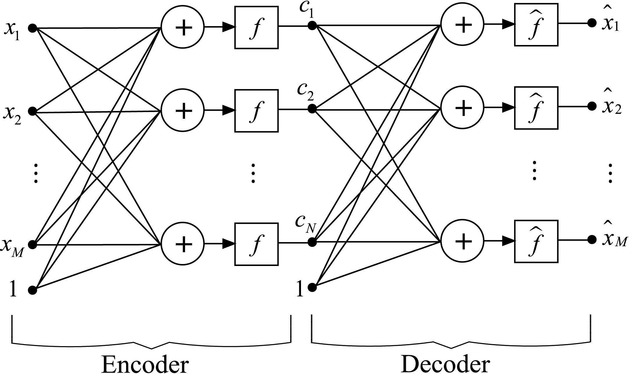The input-output relationship of the encoder is as follows [23]: $c = f (b + W^{T} x)$ (1) where c = [c₁ c₂ … c_N] ^T, which is output of the hidden layer, x = [x₁ x₂ … x_M] ^T, b = [b₁ b₂ … b_N] ^T, W = [w₁ w₂ … w_N] and f is the neuron activation function, which is generally of sigmoid type. Here the W matrix contains the weights connecting the input nodes to the neurons in the hidden layer. Therefore, each of its columns, w_i, contains the weights connecting input nodes to the ith neuron in the hidden layer: w_i = [w_i1 w_i2 … w_iM] ^T where i = 1 … N.

Fig.1

A model of the autoencoder network.

The input-output relationship of the encoder section may shortly be denoted by: $c = g_{E} (W, b; x)$ (2) where g_E may be considered as the encoding function.

The right half of the AE is called the decoder, whose input is the output of the hidden layer and output is the output of the AE. The decoder converts a given code vector into the original input vector that generated it [23].

The input-output relationship of the decoder is as follows: $\hat{x} = \hat{f} (\hat{b} + {\hat{W}}^{T} \hat{c})$ (3) where $\hat{x} = [{\hat{x}}_{1} {\hat{x}}_{2} \dots {\hat{x}}_{M}]^{T}$ , $\hat{b} = [{\hat{b}}_{1} {\hat{b}}_{2} \dots {\hat{b}}_{M}]^{T}$ , $\hat{W} = [{\hat{w}}_{1} {\hat{w}}_{2} \dots {\hat{w}}_{M}]$ and $\hat{f}$ is the neuron activation function of the neurons in the output layer, which is generally a sigmoid type function too.

Similarly, the $\hat{W}$ matrix contains the weights connecting the neurons in the hidden layer of the AE to neurons in the output layer. Therefore, each of its columns, ${\hat{w}}_{i}$ , contains the weights connecting outputs of the neurons in the hidden layer to the ith neuron in the output layer of the AE. ${\hat{w}}_{i} = [{\hat{w}}_{i 1} {\hat{w}}_{i 2} \dots {\hat{w}}_{iN}]^{T}$ where i = 1 … M.

The input-output relationship of the decoder section may shortly be denoted by: $\hat{x} = g_{D} (\hat{W}, \hat{b}; c)$ (4) where g_D may be considered as the decoding function.

Based on the definitions above, the AE may be viewed as being constructed by cascading an encoder layer and a decoding layer as illustrated in Fig. 2.

Fig.2

The block diagram of the AE network.

2.2 Training of the autoencoder

Let {x⁽¹⁾, x⁽²⁾ … x^(S)} denote theS input vectors that are to be used for training the AE discussed in the previous subsection. For any of these input vectors, the output of the AE may be computed as follows [23 –25]: $\hat{x} = g_{D} (\hat{W}, \hat{b}; g_{E} (W, b; x))$ (5) which can be expressed shortly as: $\hat{x} = g_{AE} (W, b, \hat{W}, \hat{b}; x))$ (6)

The error vector is the difference between the desired and the actual outputs: $e_{k} = x^{(k)} - {\hat{x}}^{(k)}$ (7) where k = 1, 2 … S.

Hence the total mean squared error for the AE may be calculated as: $E_{T} = \frac{1}{S} \sum_{k = 1}^{S} e_{k}^{2} + \frac{λ}{2} (\sum_{i = 1}^{N} ∥ w_{i} ∥ + \sum_{i = 1}^{M} ∥ {\hat{w}}_{i} ∥)$ (8) where λ is a regularization term (also known as a weight decay term). This term is used to prevent overfitting [23].

It is easy to observe that the E_T is a function of the internal weights of the AE: $E_{T} = E_{AE} (W, b, \hat{W}, \hat{b})$ (9)

A sparsity constraint is imposed to complete the total mean formulation and to discover interesting features on the hidden unit of the AE [23 –25]: $E_{sparse} = E_{T} + β \sum_{j = 1}^{N} KL (ρ ∥ {\hat{ρ}}_{j})$ (10) where β is the weight of the sparsity penalty term and Kullback–Leibler divergence [23 –25] given as: $KL (ρ ∥ {\hat{ρ}}_{j}) = ρ \log \frac{ρ}{{\hat{ρ}}_{j}} + (1 - ρ) \log \frac{1 - ρ}{1 - {\hat{ρ}}_{j}}$ (11) where ρ is a constant called sparsity parameter chosen by the user and ${\hat{ρ}}_{j}$ is the mean activation value of jth neuron for all training set, which may be computed as follows: ${\hat{ρ}}_{j} = \frac{1}{S} \sum_{i = 1}^{S} f_{j} (x^{(i)})$ (12)

2.3 The stacked autoencoder

The sAE network is constructed by cascading the encoder sections of a desired number of trained AEs, as illustrated in Fig. 3. By recalling the input-output relationship of the AE from the previous subsection, the input-output relationship of the sAE network with L cascaded AEs can easily be obtained as follows: $g_{SAE} = g_{E}^{1} \circ g_{E}^{2} \circ \dots \circ g_{E}^{L}$ (13)

Fig.3

A stacked autoencoder.

It should be noted that each layer of a sAE network is the encoder part of a trained AE. The decoder parts of the individual AEs are not used in the construction of the sAE network as they are only necessary for training the individual encoder layers, which will be discussed in detail later.

2.4 Softmax classifier

The softmax classifier, which is also called the multinomial logistic regression, can be used to separate multiple classes and is the advanced version of the logistic regression which can handle only two classes. Hence, the logistic regression forms the basis for the softmax classifier.

The logistic regression is a binary classifier defined as follows: $h_{θ} (x) = \frac{1}{1 + e^{- θ^{T} x}}$ (14) where θ is the parameter vector of the model which is optimized by using the following cost function [31]:

$\begin{matrix} J (θ) & = & - \frac{1}{T} ⌊ \sum_{i = 1}^{T} y^{(i)} log h_{θ} (x^{(i)}) \\ + (1 - y^{(i)}) log (1 - h_{θ} (x^{(i)})) ⌋ \end{matrix}$ (15) where y⁽ⁱ⁾ ∈ {0, 1} and $x^{(i)} \in ℝ^{N + 1}$ .

The softmax classifier has a similar structure to the logistic regression and is defined as:

$\begin{matrix} h_{θ} (x^{(i)}) \\ = [\begin{matrix} p (y^{(i)} = 1 | x^{(i)}; θ) \\ p (y^{(i)} = 2 | x^{(i)}; θ) \\ ⋮ \\ p (y^{(i)} = k | x^{(i)}; θ) \end{matrix}] \\ = \frac{1}{\sum_{j = 1}^{k} exp (θ_{j}^{(T)} x^{(i)})} [\begin{matrix} exp (θ_{1}^{(T)} x^{(i)}) \\ exp (θ_{2}^{(T)} x^{(i)}) \\ ⋮ \\ exp (θ_{k}^{(T)} x^{(i)}) \end{matrix}] \end{matrix}$ (16) where y⁽ⁱ⁾ ∈ {1, 2 … k}, k denotes the number of classes and ${θ_{1}, θ_{2}, \dots θ_{k}} \in ℝ^{N + 1}$ . The cost function of the softmax regression is derived from that of the logistic regression and given as follows:

$\begin{matrix} J (θ) & = & - \frac{1}{T} [\sum_{i = 1}^{T} \sum_{j = 1}^{k} I {y^{(i)} = j} \\ log \frac{exp (θ_{j}^{(T)} x^{(i)})}{\sum_{j = 1}^{k} exp (θ_{j}^{(T)} x^{(i)})}] \end{matrix}$ (17) where I{ * } is defined as the indicator function [31]. Training of the softmax classifier corresponds to the minimization of the cost function J (θ) by using a suitable optimization algorithm.

2.5 The deep neural network

The DNN consists of sAE and a softmax layer. The desired number of the trained AE is used to form the sAE. The softmax is a multi-class classifier, which has ability to classify the two or more classes [31]. The training of the DNN is achieved by using convenient optimization algorithm such as limited memory BFGS (L-BFGS) [18], which used in this study. The pseudo code is given in Algorithm 1 for all training procedure of the DNN. The training procedure shown in Fig. 4 is very challenging procedure and summarized as follows [23]:

The first AE is trained with an unsupervised manner and it uses the raw input data set to obtain new features from the output of the hidden layer as illustrated in Fig. 5a.

The second AE is trained with the features obtained from the first trained AE of the hidden layer’s output. This is illustrated in Fig. 5b.

The softmax layer is trained with the features generated by the second trained AE of the hidden layer’s output and output labels with a supervised manner. This is illustrated in Fig. 5c.

The training process completed by combining the encoder part of the first trained AE, the encoder part of the second trained AE and trained softmax to construct the DNN, whose weights are tuned one more time, which is illustrated in Fig. 5d.

Fig.4

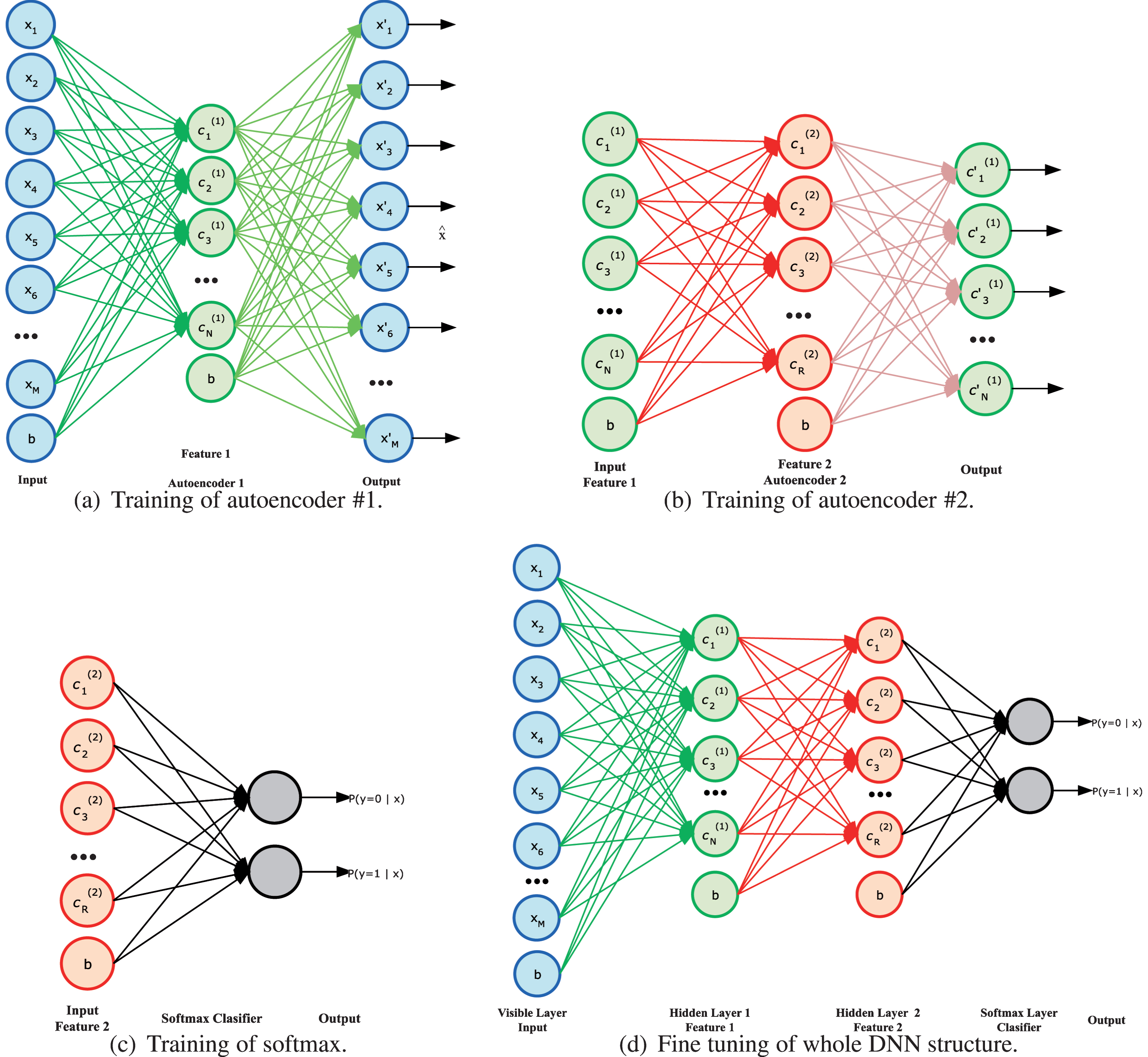
The training procedure of the DNN.

Fig.5

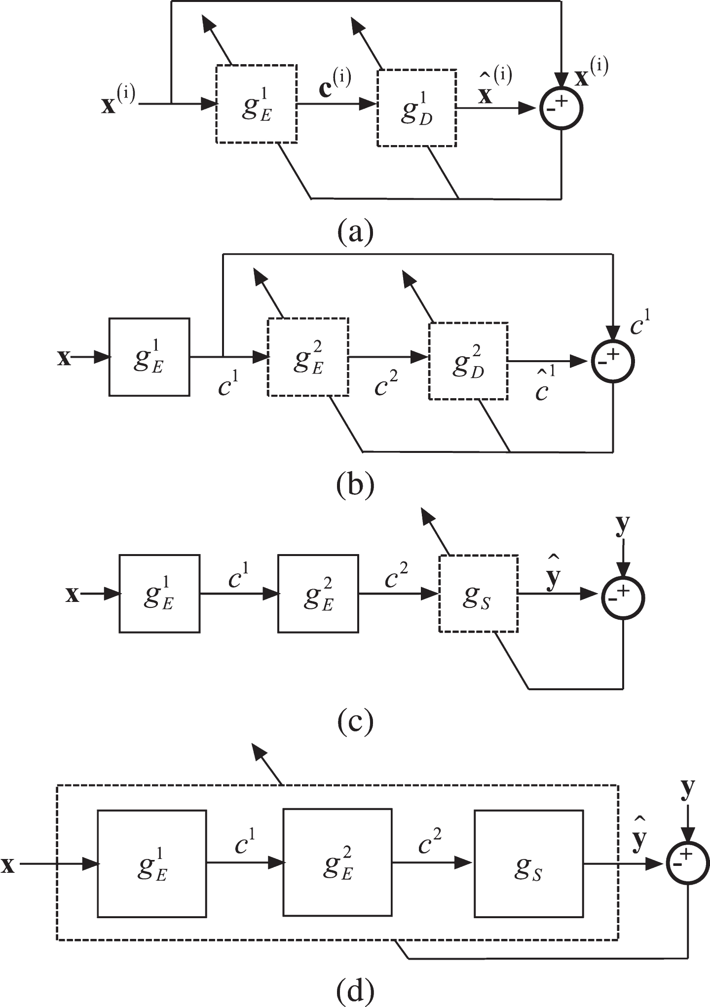
Layer by layer training of the proposed deep neural network based classification operator. (a) Training of the first encoder layer. (b) Training of the second encoder layer. (c) Training of the softmax layer. (d) Fine-tuning the whole network.

Algorithm 1

Fundamental steps of the proposed DNN.

1: Training of AE networks:

2: for t = 1 to N do

3: Train AEt with L-BFGS algorithm.

4: end for

5: Softmax:

6: Train Softmax with L-BFGS algorithm.

7: Fine-Tuning:

8: Fine-Tune DNN with L-BFGS algorithm.

2.5.1 L-BFGS optimization algorithm

The training of the DNN is achieved by using a limited number of the optimization algorithms such as L-BFGS algorithm, which is reported by Nocedal in 1980 [14]. The L-BFGS emerge to solve the problems with a high number of optimization parameters. The L-BFGS algorithm is a variant of the BFGS algorithm. This algorithm uses a different technique to predict the inverse Hessian matrix, which shows the direction of the local minima of the function.

The Hessian matrix is initialized in the first step which is iteratively corrected by the BFGS algorithm. As the number of the correction increases, the BFGS algorithm removes the oldest correction, replaces new ones due to limited memory. An user decides how many corrections (m) must be used to predict the Hessian matrix. After that, initialization of the Hessian matrix is performed to generate positive define symmetric matrix H₀, which is then used for approximating the inverse Hessian of a function (f). After H₀ is evaluated, H_k (k > m) can be found by applying m BFGS updates to H₀ using information from the m previous iterations.

Application of the L-BFGS algorithm is similar to the BFGS algorithm in the first m steps. H_k is acquired by applying m BFGS updates to H₀ using information from the m previous steps. The detailed mathematical explanation of the L-BFGS is given in Algorithm 2.

Algorithm 2
Fundamental steps of L-BFGS algorithm [18].

1: Step1. Choose x₀, m, $0 < β' < \frac{1}{2}, β' < β < 1$ and positive definite starting matrix H₀, set k = 0

2: Step2. Compute

$d_{k} = - H_{k} g_{k}$

$x_{k + 1} = x_{k} + α_{k} d_{k}$

where α_k satisfies the Wolfe conditions:

$f (x_{k} + α_{k} d_{k}) \leq f (x_{k}) + β^{'} α_{k}$

$g (x_{k} + α_{k} d_{k}) \geq β g_{k}^{T} d_{k}$

(take step length alpha_k = 1 first.)

3: Step3. Let $\hat{m} = \min (k, m - 1)$ . Update $H_{0} \hat{m} + 1$ times using pairs ${y_{j}, s_{j}}_{j = k - \hat{m}}^{k}$ i. e. let

$H_{k + 1} = (V_{k}^{T} \dots V_{k - \hat{m}}^{T}) H_{0} (V_{k - \hat{m}} \dots V_{k}) + ρ_{k - \hat{m}} (V_{k}^{T} \dots V_{k - \hat{m} + 1}^{T}) s_{k - \hat{m}} s_{k - \hat{m}}^{T} (V_{k - \hat{m} + 1} \dots V_{k}) + ρ_{k - \hat{m} + 1} (V_{k}^{T} \dots V_{k - \hat{m} + 2}^{T}) s_{k - \hat{m} + 1} s_{k - \hat{m} + 1}^{T} (V_{k - \hat{m} + 2} \dots V_{k}) ⋮ + ρ_{k} s_{k} s_{k}^{T}$

4: Step 4. Set k : = k + 1 and go to Step 2.

3 Experimental results and discussion

In this study, a DNN classifier is proposed for the classification of hyperspectral images. The proposed DNN is compared with the state-of-the-art-methods including the SVM, KNN, NB and DT classifiers over high resolution hyperspectral remote sensing data sets. All methods are run for 30 times and the average of the obtained results are compared.

3.1 The high resolution hyperspectral remote sensing data sets

The proposed DNN and compared methods are tested with 3 different high resolution hyperspectral remote sensing data sets. First data set is “the Forest Type Mapping” and is taken from UCI repository of machine learning databases [17]. The other data sets are “Salinas-A Scene Data Set” and “Pavia Centre Scene Data Set” and are obtained from Computational Intelligence, University of the Basque Country repository of Hyperspectral Remote Sensing Scenes [2].

3.1.1 Forest type mapping data set

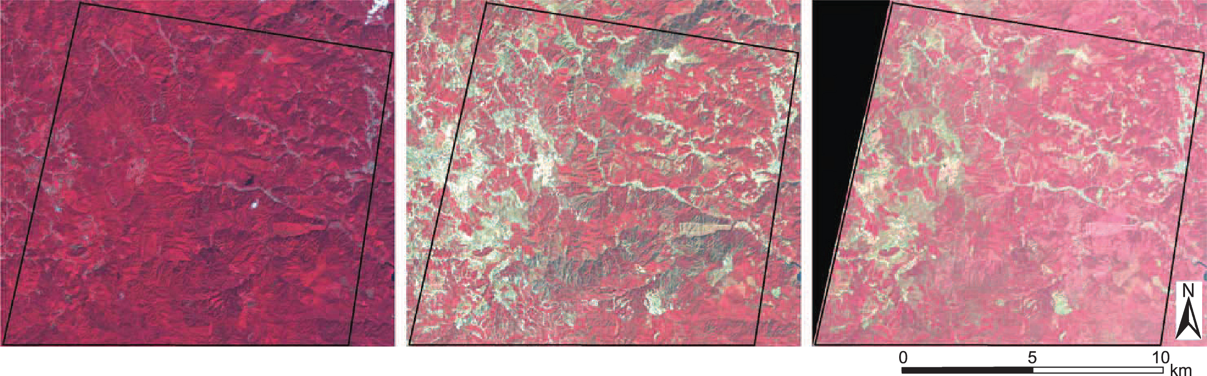
The Forest Type Mapping (Forest) data set has the high resolution hyperspectral remote sensing data, which includes approximately 13 km by 12 km forested area data in Ibaraki Prefecture in Japan. The area contains four different land cover types, two of them are the plated forest Cryptomeria Japonica (Sugi) and Chamaecyparis Obtusa (Hinoki), third one is the mixed deciduous broadleaf natural forest and the last one is different land covers such as agriculture, roads, buildings, etc. The aim of the data set is to classify the forest types by using hyperspectral data which are taken from the ASTER [1]. The data set is available in Data Mining Repository of the University of California, Irvine (UCI) [17] and is reorganized by [13]. Some examples from this data set can be seen in Fig. 6.

Fig.6

Some examples of the hyperspectral remote sensing figures from Forest data set. These ASTER false colour composite images are from an area located in Ibaraki Prefecture, Japan. Centre of this area is located at 36° 57’ N, 140° 38’ E [1, 13].

3.1.2 SalinasA Scene data set

SalinasA Scene (SalinasA) data set has been collected by the 204-band AVIRIS sensor over Salinas Valley, California. SalinasA data set is defined by high spatial resolution (3.7-meter pixels). The area covered comprises 86 × 83 pixel samples and contains six classes, namely Brocoli green weeds, Corn senesced green weeds, Lettuce romaine 4wk, Lettuce romaine 5wk, Lettuce romaine 6wk and Lettuce romaine 7wk [2].

3.1.3 Pavia Centre Scene data set

Pavia Centre Scene data set (Pavia) acquired by the ROSIS sensor during a flight campaign over Pavia, northern Italy. The number of spectral bands of Pavia is 102. The resolution of Pavia is a 1096 × 715 pixels for each band as the same time the geometric resolution of it is 1.3 meters. The Pavia data set has 9 different classes, including Water, Trees, Asphalt, Self-Blocking Bricks, Bitumen, Tiles, Shadows, Meadows and Bare Soil [2].

3.2 Simulation results

All experiments are related with random starting condition and the random ranking of the data sets, every realization of the same experiment has different results even if the experimental conditions are identical. Hence, each individual experiment performed in this paper is repeated for thirty times yielding thirty different accuracy rates for the same experiment. The averages of these accuracy rates are then taken as the representative average value for that experiment. All runs are performed on a system with 3.4 GHz Intel i7 2600 CPU and 12 GB RAM.

The proposed DNN based classifier has a few tuning parameters including the sparsity parameter (ρ), the weight decay term (λ) and the weight of the sparsity penalty term (β). Unfortunately, there is no systematical technique to decide the most convenient values for these parameters that yield the best classification performance. Therefore, the values of these parameters are heuristically determined and experimentally checked. The most optimal values of these parameters determined in this way are reported in Table 1 for each data set.

Table 1
Chosen parameter values for the proposed DNN

Phase Layer User supplied parameters Forest SalinasA Pavia

Pre-learning AE #1 Num. of Neurons 14 12 18

ρ 0.2 0.01 0.1

β 4 3 1

λ 0.003 0.003 0.003

Max iter. 1000 1000 1000

AE #2 Num. of Neurons 8 N/A N/A

ρ 0.15 N/A N/A

β 3 N/A N/A

λ 0.003 N/A N/A

Max iter. 1000 N/A N/A

SM Class 4 6 9

λ 0.003 0.003 0.003

Max iter. 1000 1000 1000

Fine Tuning Whole DNN Class 4 6 9

λ 0.003 0.003 0.003

Max iter. 1000 1000 1000

Phase	Layer	User supplied parameters	Forest	SalinasA	Pavia
Pre-learning	AE #1	Num. of Neurons	14	12	18
		ρ	0.2	0.01	0.1
		β	4	3	1
		λ	0.003	0.003	0.003
		Max iter.	1000	1000	1000
	AE #2	Num. of Neurons	8	N/A	N/A
		ρ	0.15	N/A	N/A
		β	3	N/A	N/A
		λ	0.003	N/A	N/A
		Max iter.	1000	N/A	N/A
	SM	Class	4	6	9
		λ	0.003	0.003	0.003
		Max iter.	1000	1000	1000
Fine Tuning	Whole DNN	Class	4	6	9
		λ	0.003	0.003	0.003
		Max iter.	1000	1000	1000

3.2.1 Experimental results on forest data set

The evaluation and comparison of the classification performance of the proposed DNN and the state-of-the-art-methods including SVM, KNN, NB and DT are performed over Forest data set for 30 different runs and the means and standard deviations of their accuracy rate, sensitivity and specificity rates are reported in Table 2. Besides, these obtained rates for 30 different runs are sorted and illustrated in Fig. 7a. While the experiment is realized, the data set is separated into two parts, of which 70% is employed for training and 30% for testing.

Fig.7

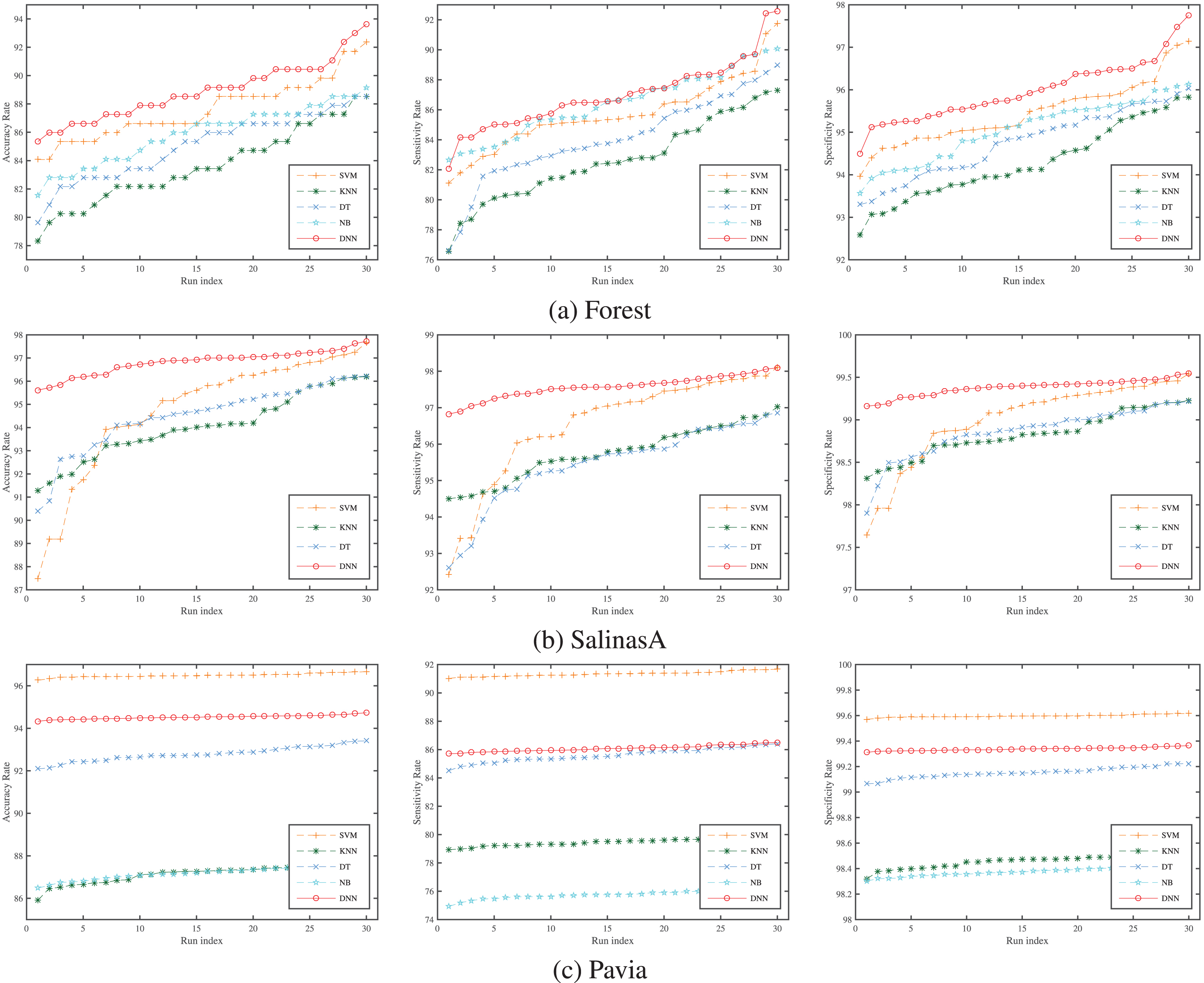
The classification performances graphics of competing methods over Forest data set for 30 runs. left: Sorted accuracy rate graphics, middle: Sorted sensitivity rate graphics, right: Sorted specificity rate graphics.

Table 2

The mean and standard deviations of the performances of competing methods on accuracy, sensitivity and specificity rates over Forest data set for 30 different runs

Method	Criteria
	Accuracy		Sensitivity		Specificity
	Mean	Std	Mean	Std	Mean	Std
SVM	87.643	2.165	85.726	2.165	95.454	0.763
KNN	83.630	2.739	82.645	2.739	94.286	0.891
DT	85.053	2.369	84.056	2.932	94.760	0.813
NB	85.881	2.062	86.387	2.196	95.059	0.731
Proposed DNN	88.896	2.087	86.986	2.284	95.979	0.730

The confusion matrix is an important tool to analyze the performance of the classification method which is utilized to compare the performances of the classification methods used in this paper. The confusion matrices for average performance valued accuracy rate of each classification method are shown in Fig. 8. All confusion matrices demonstrate that the performance of the DNN is better than the state-of-the-art methods including SVM, NB, DT and KNN.

Fig.8

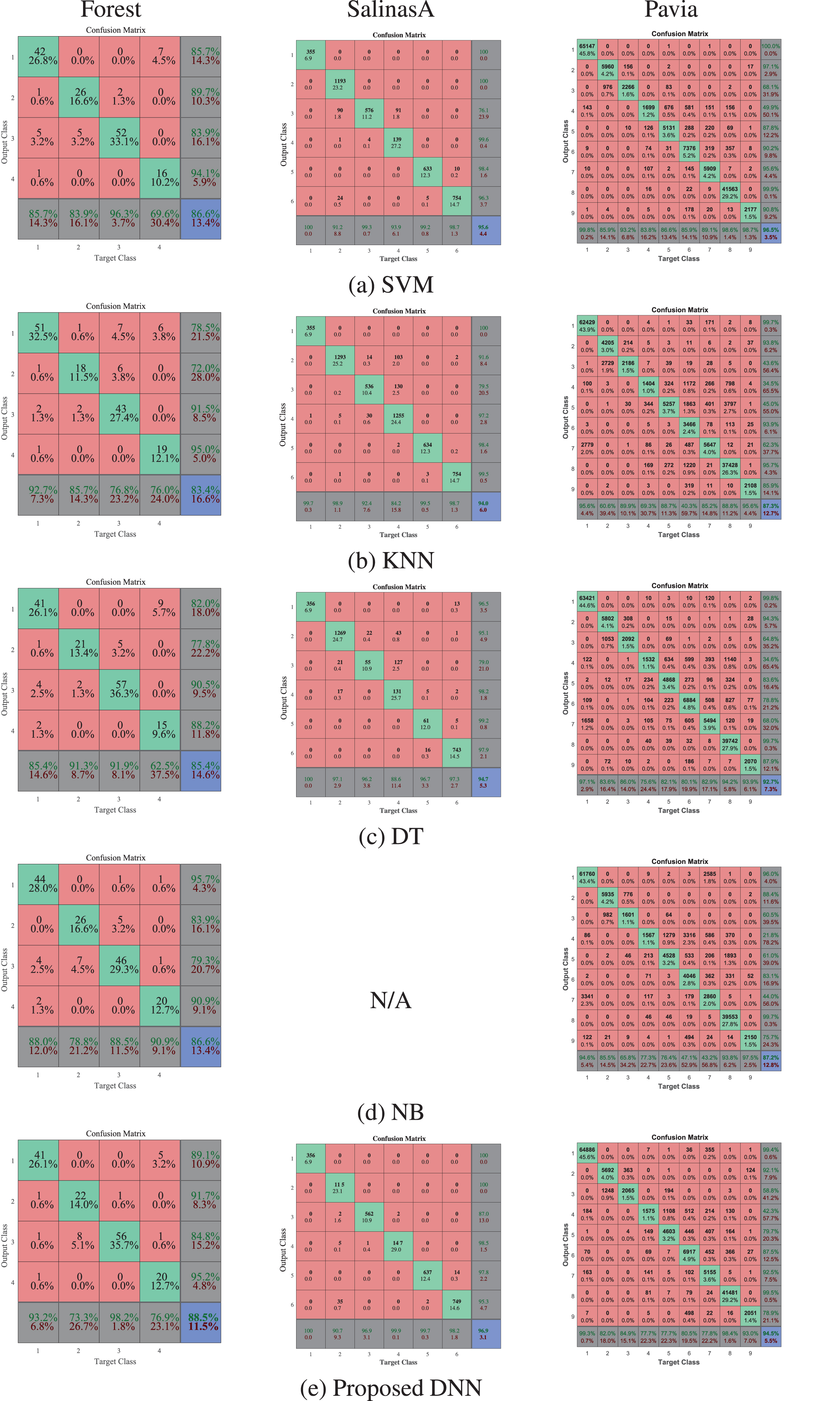
The classification average performances of the methods are presented by the confusion matrices generated using their accuracy rates over Forest, SalinasA and Pavia data set. The left, middle, and right columns show the average performance of each method over Forest, SalinasA and Pavia, respectively.

When Table 2 and Figs. 7a and 8 are investigated, it is seen that the proposed method has the best performance. As it is seen from this table and the figures, the performances of the KNN, NB and DT classification methods have nearly same classification performances, with the NB being slightly better than the DT and KNN. Besides, the SVM has the best of the state-of-the-art methods used in this study. The proposed method DNN, however, demonstrates the best classification performance of all.

Although the proposed DNN generally produces similar or better results than the others, results must be supported with statistical analyses. For this reason, Mann Whitney-U test [20] with significance level of 0.05 is conducted to compare the significance of methods to validate the performance of the proposed DNN. The results of the statistical Mann Whitney-U test are given in Table 3. The columns of the mean difference and p-value shows which one is better among two method in this table. The results of statistical analysis show that DNN is much better than the other classification methods with that p-value (p) is less than 0.05.

Table 3

The Mann-Whitney U statistical test results of competing methods over Forest data set for 30 different runs

Comparison	Mean Dif.	Z-value	p-value	Sig. (p < 0.05)
DNN-SVM	1.253	-2.253	0.024	DNN
DNN-KNN	5.266	-5.785	0.000	DNN
DNN-DT	3.843	-5.191	0.000	DNN
DNN-NB	3.015	-4.550	0.000	DNN

3.2.2 Experimental results on SalinasA data set

The classification performance of the proposed DNN and the-state-of-the-art methods, including SVM, KNN and DT are performed over SalinasA data set for 30 different runs and the means and standard deviations of their accuracy rate, sensitivity and specificity rates are reported in Table 4. Sorted values for 30 different runs are illustrated in Fig. 7b. The salinasA data set is divided as %4 training and the rest as testing parts. It is noted that, since the NB classifier is not suitable for SalinasA data set due to its nature, this classifier could not use for this data set.

Table 4
The mean and standard deviations of the performances of competing methods on accuracy, sensitivity and specificity rates over SalinasA data set for 30 different runs

Method Criteria

Accuracy Sensitivity Specificity

Mean Std Mean Std Mean Std

SVM 94.751 2.626 96.538 2.626 99.003 0.491

KNN 94.036 1.404 95.756 1.404 98.825 0.263

DT 94.483 1.468 95.460 1.109 98.854 0.299

Proposed DNN 96.817 0.531 97.564 0.317 99.380 0.098

Method	Criteria
SVM	94.751	2.626	96.538	2.626	99.003	0.491
KNN	94.036	1.404	95.756	1.404	98.825	0.263
DT	94.483	1.468	95.460	1.109	98.854	0.299
Proposed DNN	96.817	0.531	97.564	0.317	99.380	0.098

The confusion matrices for minimum, median and maximum valued accuracy rates of each classification method are shown in Fig. 8 through the left, middle, and right columns, respectively. All confusion matrices supported Fig. 7b that the performance of the DNN is better than the state-of-the-art methods.

When Table 4 and Figs. 7b and 8 are analyzed, it is clearly seen that the proposed method has the best performance. Besides, this table and these figures show that the performances of the KNN and DT have nearly same accuracy, sensitivity and specificity trends. It needs to be supported by statistical analysis in order to make these results meaningful. Therefore, the results of Mann Whitney-U statistical test are given in Table 5.

Table 5

The Mann-Whitney U statistical test results of competing methods over SalinasA data set for 30 different runs

Comparison	Mean Dif.	Z-value	p-value	Sig. (p < 0.05)
DNN-SVM	2.065	-4.156	0.000	DNN
DNN-KNN	2.781	-6.366	0.000	DNN
DNN-DT	2.334	-6.358	0.000	DNN

When the Table 5 is investigated, the statistical significance is found in terms of the proposed DNN compared with each classification method (p ≤ 0.05).

3.2.3 Experimental results on Pavia data set

The proposed DNN and the-state-of-the-art-methods, including SVM, KNN, DT and NB are differently run over Pavia data set for 30 times. The means and standard deviations of their accuracy rate, sensitivity and specificity rates are presented in Table 6. In addition, these values as sorted are given in Fig. 7c. Moreover, the %4 of Pavia data set is used as training set and the rest of this data set is utilized as testing part.

Table 6
The mean and standard deviations of the performances of competing methods on accuracy, sensitivity and specificity rates over Pavia data set for 30 different runs

Method Criteria

Accuracy Sensitivity Specificity

Mean Std Mean Std Mean Std

SVM 96.493 0.092 91.344 0.092 99.597 0.010

KNN 87.175 0.449 79.482 0.449 98.458 0.051

DT 92.793 0.349 85.611 0.491 99.154 0.041

NB 87.195 0.316 75.790 0.343 98.375 0.035

Proposed DNN 94.526 0.091 86.079 0.220 99.338 0.013

Method	Criteria
SVM	96.493	0.092	91.344	0.092	99.597	0.010
KNN	87.175	0.449	79.482	0.449	98.458	0.051
DT	92.793	0.349	85.611	0.491	99.154	0.041
NB	87.195	0.316	75.790	0.343	98.375	0.035
Proposed DNN	94.526	0.091	86.079	0.220	99.338	0.013

The confusion matrices of each classification method are illustrated in Fig. 8. These confusion matrices show that the performance of the DNN is better than the state-of-the-art methods except the SVM.

When Table 6 and Figs. 7c and 8 are analyzed, it is clearly seen that the proposed method has better classification accuracy than the KNN, DT and NB methods. However, the performance of SVM is slightly better than the proposed DNN. Besides, according to this table, the sensitivity rates of all methods have similar trends in terms of their accuracy rate. Moreover, when Table 6 is analyzed in terms of specificity rate, all methods have nearly same specificity rates.

The difference between DNN and the other classification methods may be better observed by looking at the statistical results from Table 7. The Mann Whitney U Statistical Test is applied to classification results. The DNN is compared with each classification method. We report the performance of classification methods in Table 7. When the Table 7 is investigated, the statistical significance is found in terms of the proposed DNN compared with each classification method (p ≤ 0.05) except for SVM.

Table 7

The Mann-Whitney U statistical test results of competing methods over Pavia data set for 30 different runs

Comparison	Mean Dif.	Z-value	p-value	Sig. (p < 0.05)
DNN-SVM	-1.967	-6.653	0.000	SVM
DNN-KNN	7.351	-6.653	0.000	DNN
DNN-DT	1.734	-6.653	0.000	DNN
DNN-NB	7.331	-6.653	0.000	DNN

4 Conclusion

In this paper, we propose a DNN classifier for the classification of the high resolution hyperspectral remote sensing data. The analyzing and mapping of the land cover area is very important, because of its economic and environmental values. The DNN aims to extract the hidden patterns within the hyperspectral remote sensing data by using the AEs and to distinguish different land covers including agriculture, roads, buildings, etc. by using the softmax classifier. Compared to other traditional classifiers, the DNN classifier is seen to efficiently classify the high resolution hyperspectral remote sensing data, as demonstrated by the experimental results in this paper.

References

Advanced spaceborne thermal emission and reflection radiometer (2013), https://asterweb.jpl.nasa.gov/

Hyperspectral remote sensing scenes repository. computational intelligence, university of the basque country, (2017).

Badem

, Basturk

, Caliskan

and Yuksel

M.E.

, A new efficient training strategy for deep neural networks by hybridization of artificial bee colony and limited– memory bfgs optimization algorithms, Neurocomputing 266 (2017), 506–526.

Benediktsson

J.A.

and Ghamisi

, Artech House, Spectral-Spatial Classification of Hyperspectral Remote Sensing Images (2015).

Benediktsson

J.A.

, Palmason

J.A.

and Sveinsson

J.R.

, Classification of hyperspectral data from urban areas based on extended morphological profiles, IEEE Trans. on Geoscience and Remote Sensing 43(3) (2005), 480–491.

Bengio

, Practical recommendations for gradient-based training of deep architectures, in Neural networks: Tricks of the trade (2012), Springer, pp 437–478.

Caliskan

, Badem

, Basturk

and Yuksel

M.E.

, Diagnosis of the parkinson disease by using deep neural network classifier, Istanbul University - Journal of Electrical & Electronics Engineering 17 (2017), 3311–3318.

Caliskan

, Yuksel

M.E.

, Badem

and Basturk

, A deep neural network classifier for decoding human brain activity based on magnetoencephalography, Elektronika ir Elektrotechnika 23(2) (2017), 63–67.

Caliskan

, Yuksel

M.E.

, Badem

and Basturk

, Performance improvement of deep neural network classifiers by a simple training strategy, Engineering Applications of Artificial Intelligence 67 (2018), 14–23.

10.

Delalieux

, Somers

, Haest

, Spanhove

, Borre

J.V.

and Mücher

, Heathland conservation status mapping through integration of hyperspectral mixture analysis and decision tree classifiers, Remote Sensing of Environment 126 (2012), 222–231.

11.

Ghamisi

, Plaza

, Chen

, Li

and J.

, Plaza, Advanced spectral classifiers for hyperspectral images: A review, IEEE Geoscience and Remote Sensing Magazine 5(1) (2017), 8–32.

12.

Huang

, Li

, Kang

and Fang

, Spectral– spatial hyperspectral image classification based on knn, Sensing and Imaging 17(1) (2016), 1.

13.

Johnson

, Tateishi

and Xie

, Using geographically weighted variables for image classification, Remote Sensing Letters 3(6) (2012), 491–499.

14.

Jorge

, Updating Quasi-Newton Matrices with Limited Storage, Mathematics of Computation 35(151) (1980), 773–782.

15.

LeCun

, Bengio

and Hinton

, Deep learning, Nature 521(7553) (2015), 436–444.

16.

Leslie

C.S.

, Eskin

and Noble

W.S.

, The spectrum kernel: A string kernel for svm protein classification, Pacific symposium on biocomputing (2002), in Vol. 7 pp 566–575.

17.

Lichman

, UCI Machine Learning Repository, University of California, Irvine, School of Information and Computer Sciences (2013), http://archive.ics.uci.edu/ml

18.

Liu

D.C.

and Nocedal

, On the Limited Memory BFGS Method for Large Scale Optimization, Mathematical Programming 45(1–3) (1989), 503–528.

19.

and Getoor

, Link-based classification, in ICML, Vol. 3 (2003), pp 496–503.

20.

Mann

H.B.

and Whitney

D.R.

, On a test of whether one of two random variables is stochastically larger than the other, The Annals of Mathematical Statistics (1947), 50–60.

21.

Melgani

and Bruzzone

, Classification of hyperspectral remote sensing images with support vector machines, IEEE Trans. on Geoscience and Remote Sensing 42(8) (2004), 1778–1790.

22.

Mou

, Ghamisi

and Zhu

X.X.

, Deep recurrent neural networks for hyperspectral image classification, IEEE Trans. on Geoscience and Remote Sensing 55 (2017), 3639–3655.

23.

, Sparse autoencoders CS294A Lecture Notes, Stanford Univ., USA, Stanford, CA, (2011).

24.

Ngiam

, Coates

, Lahiri

, Prochnow

, Le

Q.V.

and Ng

A.Y.

, On optimization methods for deep learning, in Proceedings of the 28th international conference on machine learning (ICML-11) (2011), pp. 265–272.

25.

Poultney

, Chopra

and Cun

Y.L.

, et al., Efficient learning of sparse representations with an energy-based model, in Advances in neural information processing systems (2007), pp. 1137–1144.

26.

Quinlan

J.R.

, C4. 5: programs for machine learning, Elsevier, 2014.

27.

Rokach

and Maimon

, Top-down induction of decision trees classifiers-a survey, Systems, Man, and Cybernetics, Part C: Applications and Reviews, IEEE Transactions on 35(4) (2005), 476–487.

28.

Shawe-Taylor

and Cristianini

, Kernel methods for pattern analysis cambridge univ, (2004).

29.

Solares

and Sanz

A.M.

, Different bayesian network models in the classification of remote sensing images, in International Conference on Intelligent Data Engineering and Automated Learning (2007), pp. 10–16.

30.

, Jia

and Xu

, Convolutional neural networks for hyperspectral image classification, Neurocomputing 219 (2017), 88–98.

31.

Zhang

, Zhang

and Chen

, Deep neural network for halftone image classification based on sparse auto-encoder, Engineering Applications of Artificial Intelligence 50 (2016), 245–255.

32.

Zhong

, Gong

, Li

and Schönlieb

C.B.

, Learning to diversify deep belief networks for hyperspectral image classification, IEEE Trans. on Geoscience and Remote Sensing 55(6) (2017), 3516–3530.