A novel car-following model considering conditional heteroskedasticity of acceleration fluctuation and driving force

2.1 Fluctuation characteristics of acceleration

Acceleration is one of the most basic variables in the process of driving. Its fluctuation characteristic can not only reflect the driver’s personal driving habit, but also can be used as an important index to study the car-following behavior. Therefore, it is very important to study the fluctuation characteristics of acceleration.

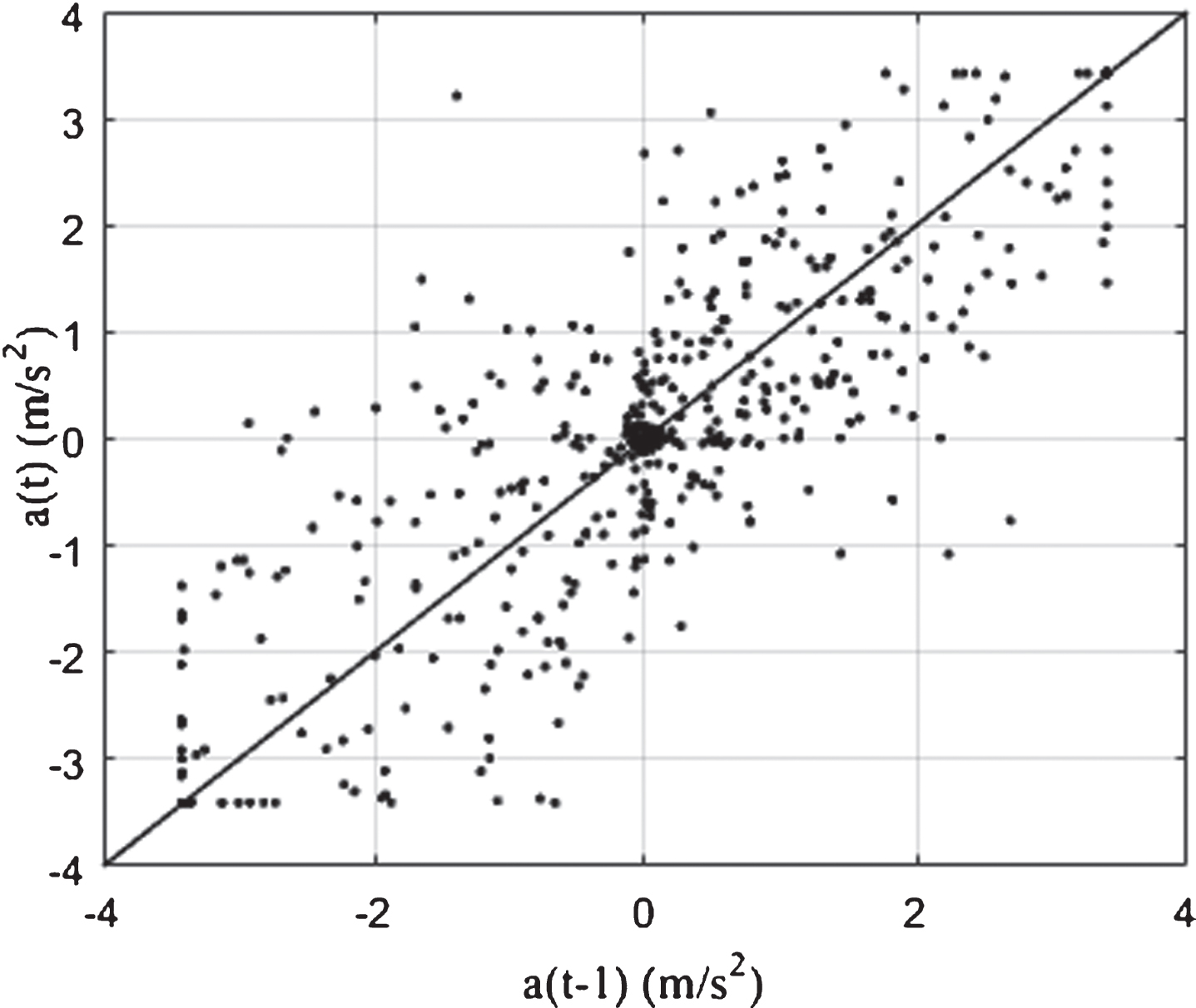
Influenced by functionality of vehicles, acceleration and deceleration is always a continuous process, and acceleration at time t fluctuates based on acceleration at time t - 1, and considering the acquisition frequency of NGSIM data is 0.1 s, so t - 1 in this paper means 0.1 s earlier. All data of NGSIM is studied, and Fig. 1 is a set of acceleration data randomly selected from our research, when the acceleration a (t - 1) is determined in the preceding period, the acceleration a (t) in the latter period changes in the range of (a (t - 1) - u _t , a (t - 1) + u _t ), where u _t is the fluctuation item affected by factors such as spacing, velocity of preceding and following vehicles, and driver’s driving habit. Figures 2 and 3 show the frequency distribution of u _t and Q-Q figure when acceleration is in the range of (–2, –1) (m/s²) and (1, 2) (m/s²). It can be seen from the Q-Q figure that the sample scatter is close to the line described by the normal distribution, so in general it can be assumed that u _t obeys a normal distribution. At the same time, effected by precision of driver’s control, u _t usually fluctuates in a certain range under the same external conditions [15, 16]. Therefore, this paper uses equation (5) to describe the fluctuation of acceleration. a n ( t ) = a n ( t - 1 ) + u t , u t ∼ N ( 0 , σ t 2 )(5)

where σ t 2 is the variance of u _t , and it changes with time.

OPEN IN VIEWER

Fig.1

Fluctuation characteristics of acceleration.

OPEN IN VIEWER

Fig.2

Frequency distribution and Q-Q figure of u _t when acceleration is in the range of (– 2, – 1) (m/s²).

OPEN IN VIEWER

Fig.3

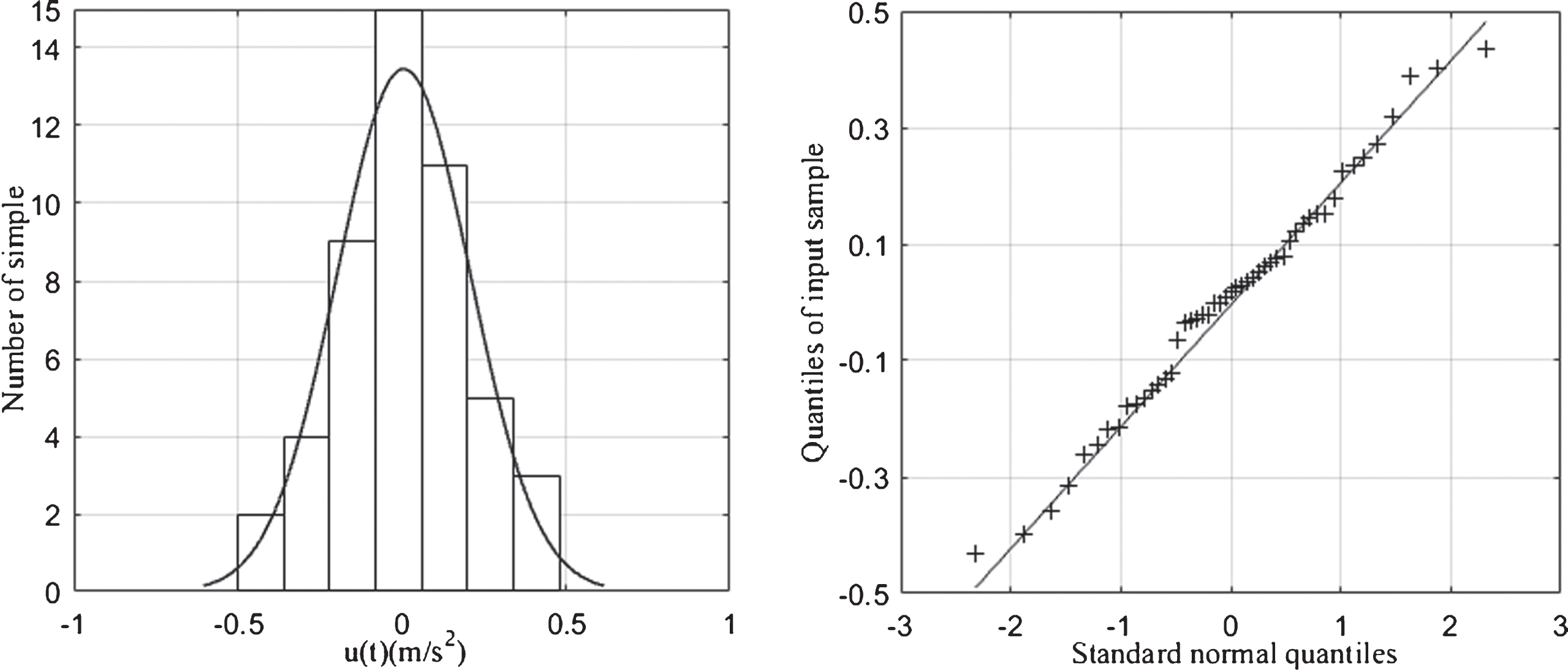
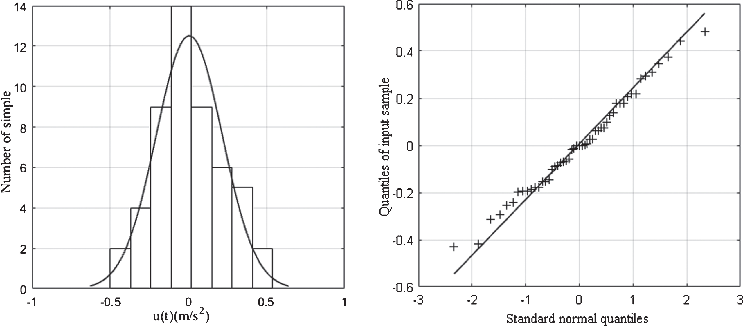
Frequency distribution and Q-Q figure of u _t when acceleration is in the range of (1, 2) (m/s²).

In the process of studying car-following behaviour, Xing [17] and Chen [18] believe that there is a desired distance between the following and preceding vehicles, that is, the spacing is always within a certain range when velocity is determined, because the driver of following vehicle always try to maintain a suitable distance which is called desired spacing. As shown in Fig. 5, when velocity is about 11 m/s, the spacing is slightly adjusted within a small range, and Weidman calls this behaviour as Oscillating processes [19]. Because drivers usually cannot accurately judge the current driving environment, and also cannot accurately maintain the pressure applied to the throttle, resulting in the actual spacing always oscillating near the desired spacing. Therefore, the desired spacing can be considered as the mean in this range and the actual spacing is evenly distributed on both sides of the desired spacing. In the actual driving process, drivers often adjust spacing according to velocity. When velocity becomes large, the driver tends to stay away from the preceding vehicle for security considerations in light of the security concerns; in contrast, when velocity becomes small, the driver tends to be close to the preceding vehicle. Therefore, velocity is the most important factors which effects spacing. The relationship between velocity and desired spacing is discussed below by the data which we chose in Section 3.1.

Average spacing under various velocity conditions is shown in Fig. 4. It can be seen from the Fig. 4 that there is a clear positive relationship between the desired spacing and velocity, which means when velocity increases gradually, the average spacing would also gradually increase. This is consistent with the reality that the driver controls spacing according to velocity. Therefore, this paper attempts to find a best equation to fit the curve (or straight line), and the results are shown in Table 1.

OPEN IN VIEWER

Fig.4

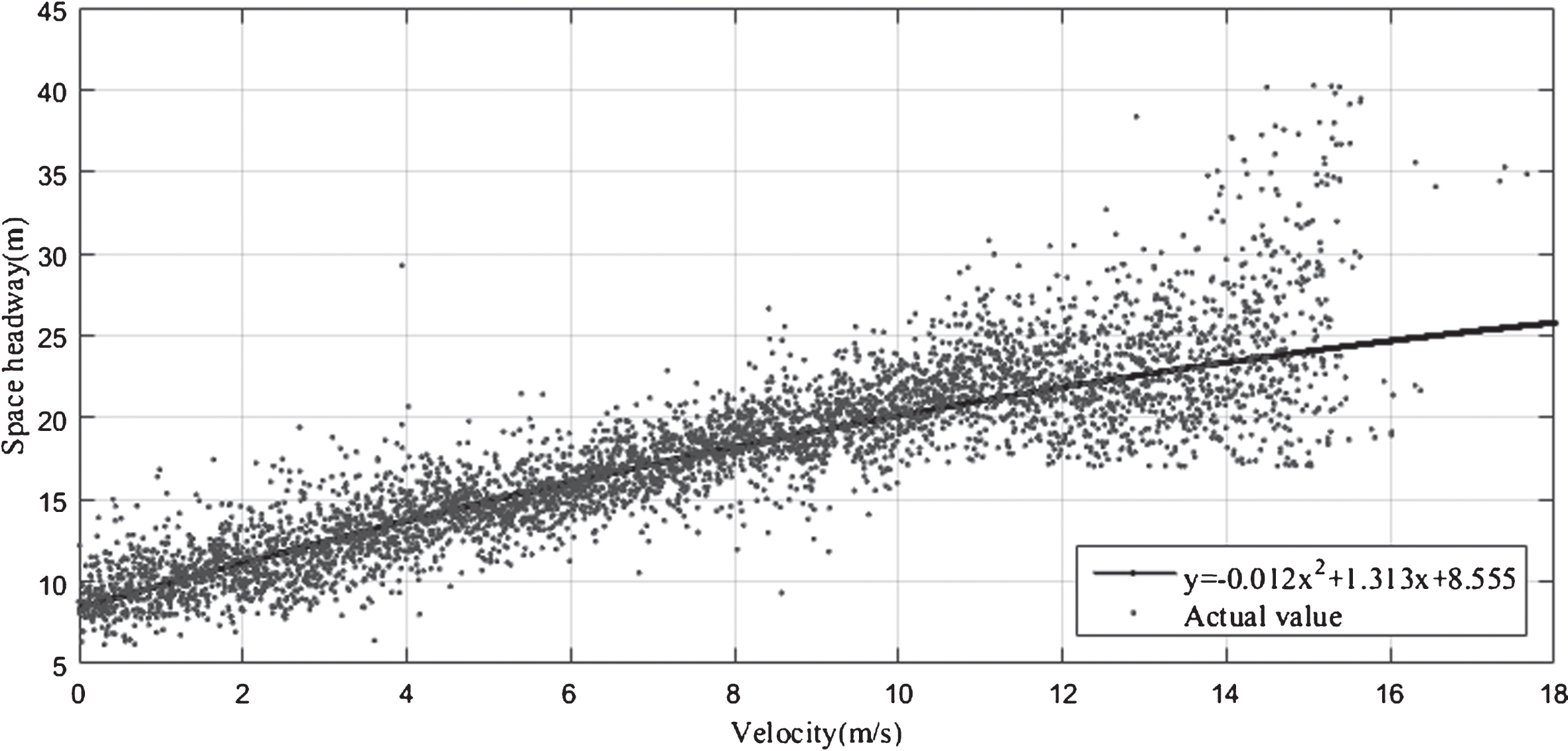
Desired spacing.

OPEN IN VIEWER

Fig.5

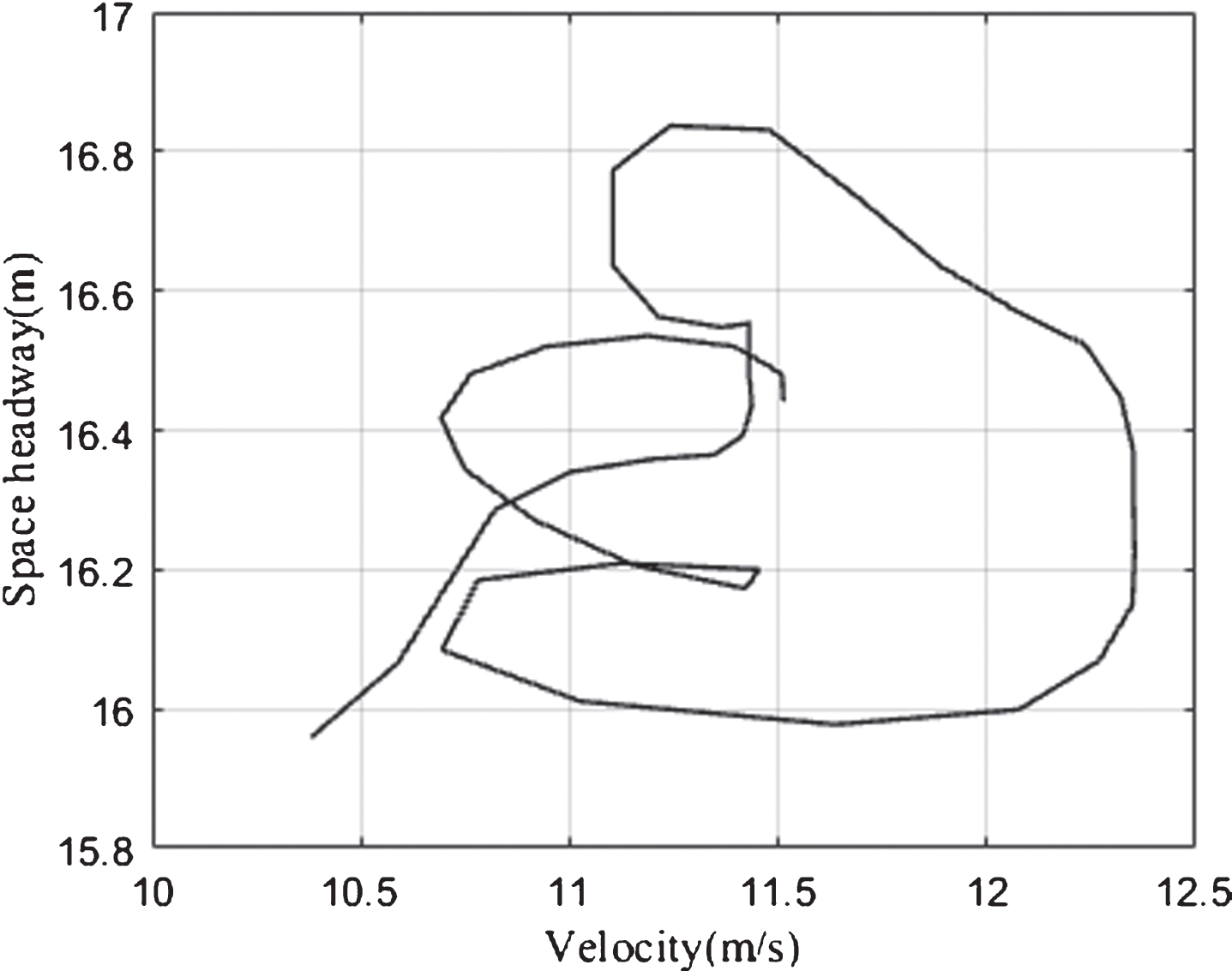
Oscillating processes of spacing when velocity is in the range of (10, 12.5) (m/s).

In fact, we have made a lot of attempts to choose a better fitting equation to fit the relation of velocity and spacing, but limited by space of paper, we can’t put all results in Table 1. According to Table 1, we can see that quadratic function can fit this relation best, and the fitting curve equation is as Equation (6). S ( t ) = - 0.012 v 2 + 1.313 v + 8.555(6)

And we will use Equation (6) as the desired spacing in the following research.

After recognizing the law of acceleration fluctuations in Section 2.1, we need to know why acceleration fluctuates. Based on the idea of classic IDM model, this paper considers the concept of the driving force and establishes the relationship. Delpiano [20] and Lin [21] have applied the concept of the driving force to the transportation field. The driving force refers to the force that helps drivers to achieve some purpose. It doesn’t act on a person’s body, but is a quantity that describes his/her motivation to take actions. In the traffic discipline, the driving force can only affect traffic participants (including drivers, riders) rather than traffic tools. Note that the driving force is very similar to social force, since both of these force correspond to social interactions. We specifically put forward the driving force concept but not borrow the generalized or social force concept directly because the driving force is more appropriate for this paper which emphasizes a person’s different motivations. The most important kinds of driving force are the efficiency force and safety force [22], which represent the driver’s motivation to improve his/her safety and efficiency respectively. However, drivers cannot know the objective value of their safety and efficiency, but they can perceive the degree to which they are safe and efficient. If the driver believes that driving is not safe enough, the safety force increases, and if the driver believes that driving efficiency is low, the efficiency force rises. The two kinds of driving force are recorded as P _efficiency and P _safety ; the car-following behaviour is the dynamic equilibrium process under the combined action of the two driving forces. P = P efficiency - P safety(7)

The driving force acts on the acceleration of the vehicle. When P _efficiency  > P _safety , the vehicle speeds up; when P _efficiency  < P _safety , the vehicle slows down; and when P _efficiency  = P _safety , the vehicle travels at an approximately constant acceleration.

In car-following behaviour, the efficiency force of the vehicle is primarily determined by the velocity of preceding and following vehicles. The following vehicle will always try to reach the destination as soon as possible. If the velocity of the preceding vehicle increases or the velocity of the following vehicle decreases, the efficiency force will increase, and then, the following vehicle would tend to accelerate consistent with the preceding vehicle; if the driving force decreases, the vehicle will slow down. The efficiency force can be defined as P efficiency = c 1 v n - 1 ( t ) v n ( t )(8)

The driver’s perception of safety is primarily affected by the spacing between the following and preceding vehicles. When spacing is less than the desired spacing, the driver of the following vehicle would feel less safe, so the safety force would be smaller; on the other hand, the safety force would be greater, so the safety driving force can be defined as P safety = c 2 S ( t ) s n ( t )(9)

In the above formulas, both c₁ and c₂ are sensitivity coefficients, and they have the effect of adjusting the dimensions and sizes of the efficiency force and safety force. S (t) is desired spacing used in this paper, and it is different from S^*, we have conduct a detailed study of it in Section 2.2. Therefore, the driving force can be defined as P t = c 1 v n - 1 ( t ) v n ( t ) - c 2 S ( t ) s n ( t )(10)

Further considering the basic characteristics of the car-following behaviour, the conditional heteroskedasticity σ t 2 of the fluctuation item u _t is affected not only by the inertia of the pre-volatility information but also by the stimulus of the preceding vehicle, both of which act on the motion state of the vehicle. Therefore, we add exogenous variables to the original GARCH model, and the novel conditional variance equation would be

σ t 2 = ω + ∑ i = 1 α i u t - i 2 + ∑ j = 1 β j σ t - j 2 + | c 1 v n - 1 ( t - 1 ) v n ( t - 1 ) - c 2 S ( t - 1 ) s n ( t - 1 ) | .(11)

The meaning of the novel conditional variance equation is as follows:

The conditional heteroskedasticity σ t 2 of u _t is affected by the driving habits of driver and the driving force.

Based on the acceleration equation and the conditional variance equation, the novel car-following model based on velocity fluctuation is as follows.

a n ( t ) = a n ( t - 1 ) + u t , u t ∼ N ( 0 , σ t 2 )(12-1)

σ t 2 = ω + ∑ i = 1 α i u t - i 2 + ∑ j = 1 β j σ t - j 2 + | c 1 v n - 1 ( t - 1 ) v n ( t - 1 ) - c 2 S ( t - 1 ) s n ( t - 1 ) |(12-2)

Before applying the GCF model, we need to verify the established model conditions. For the GARCH model, we need to know the parameter condition when the GCF model is a stationary process. Stationary process means that characteristics of its probability distribution don’t change, so we can predict σ t 2 by (12-2). Considering the consistency of properties of GARCH (1, 1) model with GARCH (i, j) model, for the sake of simplicity, it is assumed that i = 1, j = 1.

Definition 1. Time series {X _t , t = 0, ± 1, ± 2, . . .} is called stationary if for every t there is E ( X t 2 ) < ∞ and the following conditions are satisfied:

E (X _t ) is a constant independent of t;

Theorem 1. The necessary and sufficient condition for the GCF model to be a stationary process is α + β < 1 and α > 0, β > 0.

Proof. To simplify the proof process, let u t = η t σ t , η t ∼ iid N ( 0 , 1 ) .

From P = c 1 v n - 1 ( t ) v n ( t ) - c 2 S ( t ) s n ( t ) in Equation (12-2), it can assumed that F t = | P t | + ω = | c 1 v n - 1 ( t - 1 ) v n ( t - 1 ) - c 2 S ( t - 1 ) s n ( t - 1 ) | + ω .

Then σ t 2 = F t + α u t - 1 2 + β σ t - 1 2 = F t + α η t - 1 2 σ t - 1 2 + β σ t - 1 2 = F t + ( α η t - 1 2 + β ) σ t - 1 2 = F t + ( α η t - 1 2 + β ) ( F t - 1 + α u t - 2 2 + β σ t - 2 2 ) ⋮ = ∑ k = 1 ∞ [ F t - k ∏ r = 1 k ( α η t - r 2 + β ) ]

Let H ( t , k ) = ∏ r = 1 k ( α η t - r 2 + β ) . Since η t 2 is i.i.d, and the moment of H (t, k) do not depend on t, thus, we can know E (H (t, k + 1)) = (α + β) E (H (t, k)) and E (H (t, k)) = (α + β)  ^k . E ( ∑ k = 1 n H ( k , t ) ) = ∑ k = 1 n E ( H ( k , t ) ) = 1 - ( α + β ) n 1 - ( α + β )

Since η t 2 is also independent and identically distributed and satisfies E ( η t 2 ) = 1 , cov ( F t - k , H ( t , k ) ) = 0 . E ( u t 2 ) = E ( η t 2 σ t 2 ) = E { ∑ k = 1 ∞ F t - k H ( t , k ) } = ∑ k = 1 ∞ E ( F t - k H ( t , k ) ) = ∑ k = 1 ∞ ( E ( F t - k ) E ( H ( t , k ) ) )

It is easy to see that E (F_t-k)< ∞, and for a particular vehicle, E (F_t-k) is a constant c _n .

If and only if 0 < α + β < 1, E ( u t 2 ) = c n ∑ k = 1 ∞ E { H ( t , k ) } = c n 1 1 - α - β .

Therefore, u t 2 converges almost everywhere.

At the same time, both E (u _t ) =0 and cov (u _t , u _s ) =0 (t ≠ s) hold. Therefore, theorem 1 is proven. The condition for the GCF model to hold is 0 < α + β < 1.

To better use GCF model to describe and determine traffic conditions, we will further explore the properties of the model and its parameters.

Property 1. The current fluctuation of acceleration is influenced by the driving force and fluctuation values of the past period, and it decreases with increasing time interval.

Proof. σ t 2 = | c 1 v n - 1 ( t - 1 ) v n ( t - 1 ) - c 2 S ( t - 1 ) s n ( t - 1 ) | + ω + α u t - 1 2 + β σ t - 1 2 = | c 1 v n - 1 ( t - 1 ) v n ( t - 1 ) - c 2 S ( t - 1 ) s n ( t - 1 ) | + ω + α u t - 1 2 + β { c 1 v n - 1 ( t - 2 ) v n ( t - 2 ) - c 2 S ( t - 2 ) s n ( t - 2 ) + ω + α u t - 2 2 + β σ t - 2 2 } ⋮ = ∑ k = 1 ∞ β k - 1 ( | c 1 v n - 1 ( t - k ) v n ( t - k ) - c 2 S ( t - k ) s n ( t - k ) | + α u t - k 2 ) + ω 1 - β

From Property 1, we can see that the variance of the acceleration fluctuations is mainly affected by the current and past driving force and the value of the acceleration fluctuation. We know that 0 < β < 1 in Theorem 1, showing that the influence of the driving force and acceleration fluctuation on the velocity variance is smaller as time elapses. Property 1 reflects the gradual decline of the memory of vehicle acceleration fluctuation.

Property 2. The velocity fluctuation term { u t 2 } satisfies the ARMA (1, 1) model, the current acceleration fluctuation is related to the previous period, and the persistence of the fluctuation is influenced by the value of α + β.

Proof. Let δ t = u t 2 - σ t 2 , so u t 2 = | c 1 v n - 1 ( t - 1 ) v n ( t - 1 ) - c 2 S ( t - 1 ) s n ( t - 1 ) | + ω + α u t - 1 2 + β ( u t - 1 2 - δ t - 1 ) + δ t = | c 1 v n - 1 ( t - 1 ) v n ( t - 1 ) - c 2 S ( t - 1 ) s n ( t - 1 ) | + ω + ( α + β ) u t - 1 2 + δ t - β δ t - 1

That is, u t 2 satisfies the ARMA (1, 1) model, and there is autocorrelation. The persistence of fluctuation is mainly determined by the value of α + β, and the closer α + β is to 1, the greater the persistence of fluctuation. In the actual car-following situation, the bigger α + β is, the more the fluctuation of the previous period will affect the fluctuation of the current acceleration, while the value of α + β is mainly affected by the driver’s driving habits and character.

Property 3. No bias estimation of the square of acceleration change value g t 2 is σ t 2 .

Proof. Based on u t ∼ N ( 0 , σ t 2 ) , we can learn that: E ( ( a t - a t - 1 ) 2 ) = E ( g t 2 ) = E ( u t 2 ) = E ( ( u t - 0 ) 2 ) = E ( σ t 2 ) = σ t 2

Therefore, the corresponding conditional heteroskedasticity σ t 2 can be used as an estimate of the square of acceleration change value g t 2 . At the same time, it can be known from the definition of conditional heteroskedasticity that its value is predicted by information before time t. So from Property 3, the value of g t 2 can be predicted forward.

3.1 Data collection

The data source is the next-generation simulation project NGSIM by the United States Federal Highway Administration. The data are collected at Highway 101, Los Angeles, California, USA, from 8:05 to 8:20 am. The target is the driving condition of all the vehicles that meet the car-following behaviour of the section.

The length of the road is approximately 640 metres, and there are five main lanes and an auxiliary lane. As the acquisition time for the traffic is from the early peak to peak recovery, traffic density is relatively moderate, with the occurrence of car-following behaviour more universal. The acquisition method is to use a camera near the road that detects video images. A continuous state of motion information of individual vehicles is recorded and entered into the database. A total of eight cameras are installed along the way and numbered 1 to 8, and their distribution is shown in Fig. 1. Image data are collected by these eight cameras; the acquisition frequency is 10 frames per second. Numbering of the vehicle is automatic when the vehicle enters the range of the 1/8 camera (according to the time of entering the observation area). The vehicle operating conditions are recorded until the vehicle is out of range of the 8/1 camera. The system automatically records vehicle information, including the velocity and acceleration of the following vehicle, number of preceding and following vehicles and other parameters.

In order to ensure that the data is reasonable and the research is accurate, this paper uses the following rules to select the appropriate data:

Select all vehicles of the third lane which possess more car-following characteristics, except for the first vehicle;

Through the above criteria of data screening, a total of 72 sets of data are selected, the following research will focus on these data.

3.2 Heterogeneity test

The basic assumption of the model (5) is that the conditional variance of the fluctuation term of acceleration is affected by the preceding vehicle and varies with time, in other words, there is heteroskedasticity. Therefore, before fitting the data with (12), we need to verify the existence of heteroskedasticity (ARCH effect).

Use equation (5) to fit the acceleration of the following vehicle, and obtain the fluctuation term in Fig. 6. It can be seen that there is an aggregation effect of the fluctuation, which means that the fluctuation is small in some time periods and very large in other time periods, indicating that the fluctuation term may meet heteroskedasticity. To confirm the existence of heteroskedasticity, the Lagrange multiplier rule is used to test the heteroskedasticity.

OPEN IN VIEWER

Fig.6

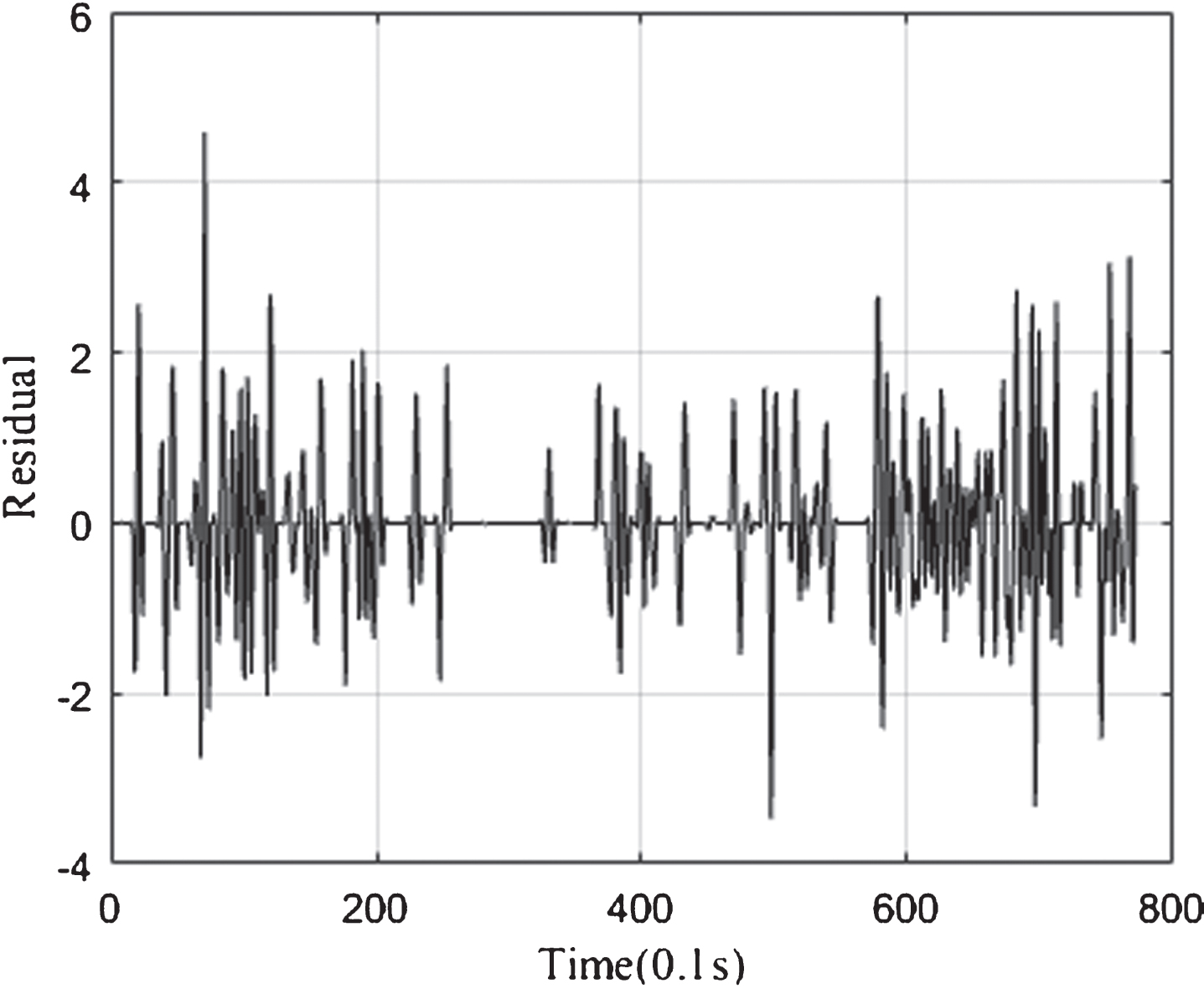
Residual term u _t .

The hypothesis of the Lagrange multiplier rule is that there is no ARCH effect until order p of the residual sequence. The value of P in (Table 2) is 0 significantly, so the hypothesis is rejected and the sequence {u _t } has significant heteroskedasticity.

For GCF model, after verifying the existence of heteroskedasticity of the acceleration fluctuation term series, the car-following data can be further fitted by Equation (12). According to the Property 3, we can predict the square of one order difference value of acceleration by σ t 2 . For IDM model, this paper chooses genetic algorithm (GA) method to estimate related parameters. Matlab and genetic algorithm toolbox are used as simulation tools, then the initial population number is set to 20, no improvement stop algebra is set to 50. When acceleration a _n  (t) of IDM model is estimated, the square of the first order difference of acceleration can be calculated easily.

The comparison of actual values and predicted values of IDM model and GCF model is as following Fig. 7 (the length of data is limited to 400*0.1 s to ensure recognition of Fig. 7). In Fig. 7, there are three groups of experiment fitting results selected by fluctuating frequency and amplitude. After comparison, the peak time and the frequency of fluctuation of GCF model are both found to be in basic agreement, and the amplitude of fluctuation is closer than IDM model. Therefore, it can be preliminary concluded that the GCF model established by the dynamic balance of two driving forces can effectively fit the fluctuation of acceleration. It can also be found that the predicted value of GCF is often lower than the actual value at the time when the acceleration fluctuation is abnormally increasing, mainly because when velocity of the preceding vehicle falls sharply, driver of the following vehicle will overreact, which means that driver will take a bigger deceleration, but the GCF model cannot take it into account. On the other hand, it can be seen from Fig. 7 that it doesn’t affect the overall prediction of acceleration of GCF model, it is mainly because the memory of GCF model can simulate the driver’s driving habits.

OPEN IN VIEWER

Fig.7

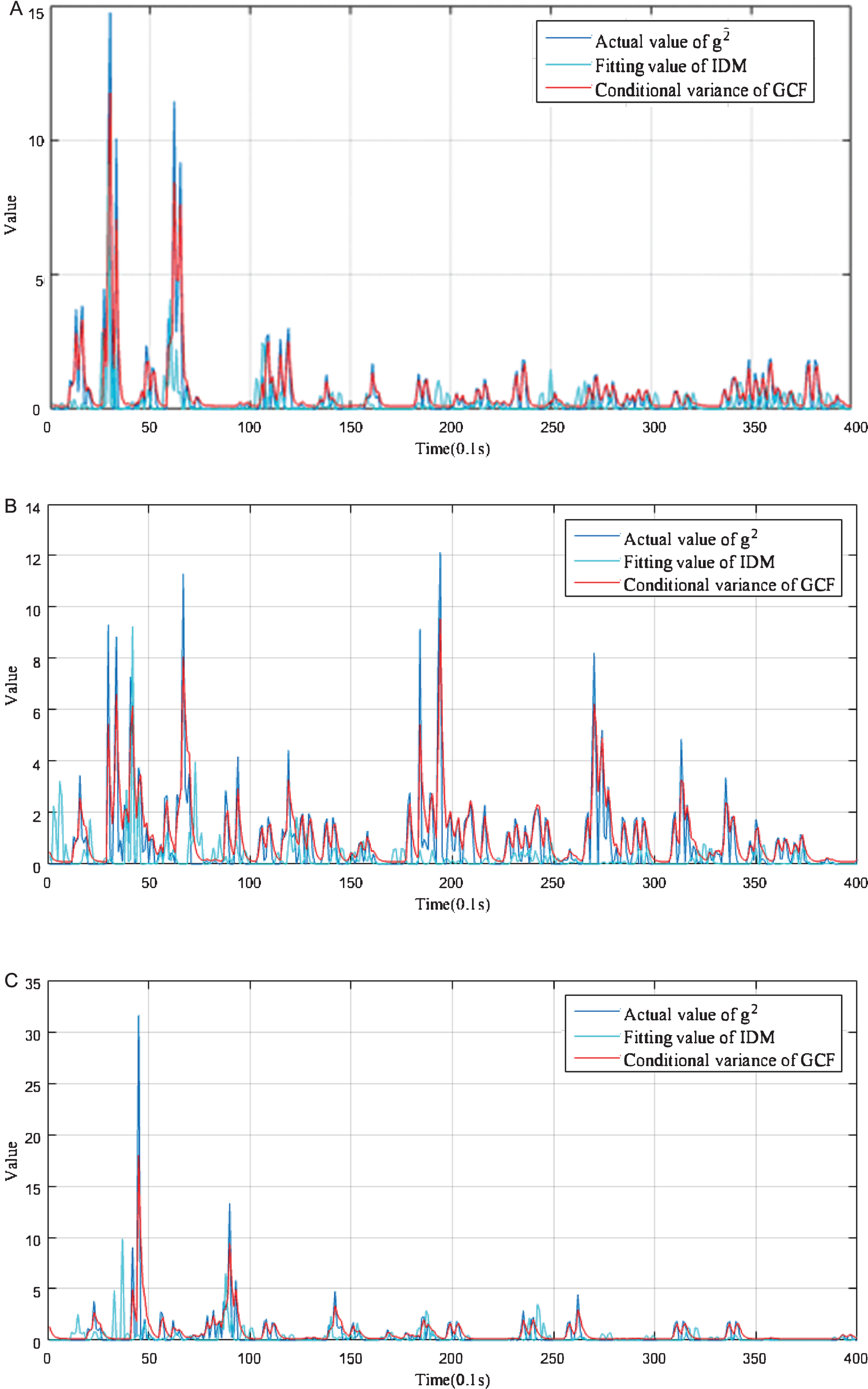
Comparison of predicted and actual values of g t 2 . (a) Number of following vehicle is 1602. (b) Number of following vehicle is 1668. (c) Number of following vehicle is 1748.

Taking into account that the predicted results of the GCF model is good, so we think that it can play the role of security warning. Such as the vehicle 1748, its acceleration fluctuation is gentler than the vehicle 1602 and the vehicle 1668 for most of time, but at 65*0.1 s, the predicted value and actual value are rising violently, and there is a big security risk in this situation, thus, it is possible to provide an early warning to the driver when the GCF model predicts a large increase in fluctuation and then prevent further increase. On the other hand, after comparing the fluctuation feature of vehicles above, it can be found that the fluctuation of the vehicle 1602 and the vehicle 1748 is gentler than vehicle 1668, and the times that the fluctuation value of the vehicle 1668 is greater than 6 is more, so it is obvious that the driver of the vehicle 1668 may be an aggressive driver. Therefore, we can conclude that drivers should be reminded to drive carefully when the GCF model predicted bigger fluctuation continuously.

In order to compare the accuracy of GCF model with it of IDM model, we need to select an error analysis function. Considering that acceleration fluctuation could be 0, we use MSE (Mean Squared Error) function to analyse the accuracy of the two models. MSE = 1 n ∑ t = 1 n ( O t - P t ) 2(14) where O _t is observed value and P _t is predicted value.

The two models are used to fit the data respectively which we screen out in Section 3.1, and the corresponding acceleration fluctuation term is obtained. Finally, compare the accuracy of the two models respectively based on the MSE function.

From the results of Table 3, we can find that the MSE error function value of GCF model is obviously lower than that of IDM model and most of the values is less than 1, so it can be indicated that GCF model can describe the fluctuation of acceleration better. It is mainly affected by the form of IDM, because IDM model is set to avoid impractical acceleration and deceleration, in other word, both of the maximum acceleration a and comfortable deceleration b of IDM are less than actual maximum acceleration and deceleration [23, 24], so it results that the acceleration fitted by IDM model to be significantly lower than actual acceleration, and cannot reflect the real-time change of acceleration. But the GCF model proposed in this paper is based on the idea of IDM model and considering the personal driving habit of the driver in the past, so it is more realistic to reflect the fluctuation characteristics of acceleration. Thus the fitting effect of acceleration fluctuation may be obviously better than that of IDM model.