A multi-item generalized intuitionistic fuzzy inventory model with inventory level dependent demand using possibility mean,variance and covariance

Abstract

Generalized intuitionistic fuzzy numbers (GIFNs), a special kind of intuitionistic fuzzy set (IFSs) on the real number set are useful to deal with ill-known quantities in fuzzy optimization problems. How to measure the value and uncertainty of a GIFN is of eminent importance. The earlier part of the paper describes the concept of the possibility mean, variance and covariance of generalized intuitionistic fuzzy number. Furthermore, we show that possibility mean and variance of linear combination of generalized intuitionistic trapezoidal fuzzy numbers can be computed in a conventional way to those probability theory. Another part of this paper investigates a multi-item inventory model with inventory level dependent demand in generalized intuitionistic fuzzy environment. By employing the possibility mean and variance, the multi-item generalized intuitionistic fuzzy inventory model (MGIFim) is transformed into an equivalent deterministic linear programming problem. Finally, the model is illustrated with the help of numerical example, and to validated the proposed model few sensitivity analyses are also presented under different parameters.

Keywords

Generalized intuitionistic fuzzy number possibility mean & variance multi-items inventory level dependent demand

1 Introduction

Fuzzy set theory has been well exhibited and applied in a wide variety of real problems since it was proposed in 1965 by Zadeh [1]. Zadeh [1] expresses the degree of membership of a given element in a fuzzy set, but very often does not express the corresponding degree of non-membership as the complement to 1. Thus, Atanassov [2] introduced the intuitionistic fuzzy set(IFS) by adding an additional non-membership function, this may express more enormous and supple information as compared with the fuzzy set. The IFS has an eminent characteristic which allots to each element a membership degree and a non-membership degree. Intuitionistic fuzzy numbers are a special instance of fuzzy numbers. As a generalization of fuzzy Set, the intuitionistic fuzzy number (IFN) is a special kind of IFS defined on the real number set, which appears to properly describe an ill-known quantity [33]. At present now, there are three kinds of emblematic IFNs: triangular IFN(TrIFN) [5, 6], trapezoidal IFN(TIFN) [4, 7] and inter-valued trapezoidal IFN [3, 8], which have enticed much research interest currently.

The possibility theory of fuzzy set was introduced by Zadeh [9] and developed by many researchers, e.g. Dubois and Prade [10], Yager [12], Klir [11] and others. The possibility mean and variance are the significant mathematical prominence of fuzzy numbers. The notations of lower and upper possibilistic mean were introduced by Carlsson and Fuller [14]. They also define the interval-valued possibilistic mean and investigate its relationship to the interval-valued probabilistic mean. Fuller and Majlender [13] introduced the notation of weighted interval-valued possibilistic mean value of fuzzy numbers and investigate its relationship to the interval-valued probabilistic mean. Recently, Wan et al. [15] introduced the possibility mean, variance and covariance of TrIFNs. A correlation coefficient of generalized intuitionistic fuzzy sets with statistical method was introduced by Park et al. [34]. Using a citation network analysis, Yu and Shi [40] have developed the Atanassov intuitionistic fuzzy set. Several research like as: Dejian and Huchang [39], Panigrahi and Nanda [35], Gagr [29], Zhou and He [36], Zhao et al. [37], Garg and Ansha [27] and Zhou et al. [38] are studied on intuitionistic fuzzy set theory and its different applications.

The inventory problem is an expansion that has received important attention in inventory models with stock dependent demand, time-varying demand and partial backlogging. Gupta and Vart [16] were the first to developed an inventory model for stock-dependent consumption rates. Wu et al. [17] presented an inventory model for non-instantaneous deteriorating items with backlogging and stock dependent demand. In the past decades, many researches studied on backlog. Padmanabhan and Vrat [18] presented an inventory model with complete backlogging and partial backlogging. Examples of other studies in this area encircle Chang [19], Dye [20], Garai et al. [28] and Chang et al. [21]. A multi-objective non-linear programming problem in the intuitionistic fuzzy environment was developed by Rani et al. [26]. Gagr [31] presented an Inventory model involving variable lead time, backorder discounts and lost sales using PSO. Recently, Lee and Dye [22] formulated an inventory model for deteriorating items with stock dependent demand and partially backlogged. Other studies in this area include those of Valliathal and Uthayakumar [25], Gagr [30], Tripathi [24], and Pando et al. [23]. However, there was no investigation on possibility mean, variance and covariance of GTIFNs. The aim of this article is to define the possibility mean and variance of GTIFNs, and apply to the multi-item generalized intuitionistic fuzzy inventorymodel.

In spite of the above mentioned developments, following additions can also be made in generalized intuitionistic fuzzy numbers, the formulation and solution of multi-item inventory model with inventory level dependent demand under GTIFNs environments.

Possibility mean, variance and covariance of generalized intuitionistic fuzzy number.

Possibility mean, variance and covariance of generalized trapezoidal intuitionistic fuzzy number.

Multi-item inventory model with inventory level dependent demand under GTIFNs environments.

Possibilistic mean, variance methods to solve Multi-item intuitionistic fuzzy inventory model.

The rest of the paper is organized as follows: In Section 2, we present some basic knowledge of GIFNs, and gives also the concepts of possibility mean, variance and covariance of GIFNs. In Section 3, we formulate the possibility mean, variance and covariance of GTIFNs. In Section 4, we introduce the notations used throughout the paper and the assumptions of MGIFim. In Section 5, A multi-item inventory problem has been developed in GTIFN environment and discuss also its two solution methods. The numerical examples are illustrated in Section 6. In Section 7, the result of change in different parameters are discussed graphically. Finally, the conclusion and scope of future work plan affair in Section 8.

2 Basic preliminaries

Definition 2.1. Let $w_{\tilde{a}} \in [0, 1]$ and $u_{\tilde{a}} \in [0, 1]$ be any two real numbers $ℝ$ , which satisfy that $0 \leq w_{\tilde{a}} + u_{\tilde{a}} \leq 1$ . A generalized intuitionistic fuzzy(GIFN) number ${\tilde{a}}^{I}$ is a special type intuitionistic fuzzy set [4] on the set of real number $ℝ$ , whose membership function and non membership function are $μ_{{\tilde{a}}^{I}} : ℝ ⟶ [0, w_{\tilde{a}}]$ and $ν_{{\tilde{a}}^{I}} : ℝ ⟶ [u_{\tilde{a}}, 1]$ respectively, which are satisfies the following conditions (1) ↔ (4).

∃ at least two real number x₁ and x₂ such that $μ_{{\tilde{a}}^{I}} (x_{1}) = w_{\tilde{a}}$ and $ν_{{\tilde{a}}^{I}} (x_{2}) = u_{\tilde{a}}$ .

$μ_{{\tilde{a}}^{I}}$ is a upper semi continuous and quasi concave on the real number $ℝ$ .

$ν_{{\tilde{a}}^{I}}$ is a lower semi continuous and quasi convex on the real number $ℝ$ .

the support of ${\tilde{a}}^{I} (i . e {\tilde{a}}_{< 0, 1 >}^{I} = {μ_{{\tilde{a}}^{I}} (x) \geq 0, ν_{{\tilde{a}}^{I}} (x) \leq 1; \forall x \in ℝ})$ is bonded.

From the above definition of the generalized intuitionistic fuzzy number, we can easily construct a generalized intuitionistic fuzzy number ${\tilde{a}}^{I} = {(\underline{a_{1}}, a_{1 l}, a_{1 r}, \bar{a_{1}}); w_{\tilde{a}}, (\underline{a_{2}}, a_{2 l}, a_{2 r}, \bar{a_{2}}); u_{\tilde{a}}}$ whose membership and non membership functions are given by $μ_{{\tilde{a}}^{I}} (x) = {\begin{matrix} 0 & if x < \underline{a_{1}} \\ g_{μ l} (x) & if \underline{a_{1}} \leq x < a_{1 l} \\ w_{\tilde{a}} & if a_{1 l} \leq x \leq a_{1 r} \\ g_{μ r} (x) & if a_{1 r} < x \leq \bar{a_{1}} \\ 0 & if x > \bar{a_{1}} \end{matrix}$ and $ν_{{\tilde{a}}^{I}} (x) = {\begin{matrix} 1 & if x < \underline{a_{2}} \\ g_{ν l} (x) & if \underline{a_{2}} \leq x < a_{2 l} \\ u_{\tilde{a}} & if a_{2 l} \leq x \leq a_{2 r} \\ g_{ν r} (x) & if a_{2 r} < x \leq \bar{a_{2}} \\ 1 & if x > \bar{a_{2}} \end{matrix}$ respectively. Where the functions $g_{μ l} : [\underline{a_{1}}, a_{1 l}] \to [0, w_{\tilde{a}}]$ and $g_{ν r} : [a_{2 r}, \bar{a_{2}}] \to [u_{\tilde{a}}, 1]$ are continuous, non decreasing and satisfy the conditions $g_{μ l} (\underline{a_{1}})$ = 0, $g_{μ l} (a_{1 l}) = w_{\tilde{a}}$ , $g_{ν r} (a_{2 r}) = u_{\tilde{a}}$ and $g_{ν r} (\bar{a_{2}}) = 1$ ; the functions $g_{μ r} : [a_{1 r}, \bar{a_{1}}] \to [0, w_{\tilde{a}}]$ and $g_{ν l} : [\underline{a_{2}}, a_{2 l}] \to [u_{\tilde{a}}, 1]$ are continuous, non increasing and satisfy the conditions $g_{μ r} (a_{1 r}) = w_{\tilde{a}}, g_{μ r} (\bar{a_{1}}) = 0$ , $g_{ν l} (\underline{a_{2}}) = 1$ and $g_{ν l} (a_{2 l}) = u_{\tilde{a}}$ . $\bar{a_{1}}$ and $\underline{a_{1}}$ are called upper and lower limits and [a_1l, a_1r] be called the mean interval of the generalized intuitionistic fuzzy number ${\tilde{a}}^{I}$ for the membership function respectively. $\bar{a_{2}}$ and $\underline{a_{2}}$ are called the upper and lower limits and [a_2l, a_2r] be called the mean interval of the generalized intuitionistic fuzzy number ${\tilde{a}}^{I}$ for the non membership function respectively. $u_{\tilde{a}}$ and $w_{\tilde{a}}$ are called the minimum non-membership and maximum membership degree respectively. Then further we can construct some specific forms of generalized intuitionistic fuzzy numbers such as generalized trapezoidal intuitionistic fuzzy number and generalized triangular intuitionistic fuzzy number. For some particular values $\overset{´}{a_{1}}, a_{1}, a_{2}, a_{3}, a_{4}$ and $\overset{´}{a_{4}}$ of the parameters $\underline{a_{1}}, a_{1 l}, a_{1 r}, \bar{a_{1}}, \underline{a_{2}}, a_{2 l}, a_{2 r}$ and $\bar{a_{2}}$ (with a_1l = a_2l, a_1r = a_2r) respectively.

Definition 2.2. Let ${\tilde{a}}^{I}$ be an intuitionistic fuzzy number [7] in the set of real numbers $ℝ$ , whose membership function and non-membership function are defined as follows: $μ_{{\tilde{a}}^{I}} (x) = {\begin{matrix} \frac{x - a_{1}}{a_{2} - a_{1}} w_{\tilde{a}}, & if a_{1} \leq x < a_{2} \\ w_{\tilde{a}}, & if a_{2} \leq x \leq a_{3} \\ \frac{a_{4} - x}{a_{4} - a_{3}} w_{\tilde{a}}, & if a_{3} < x \leq a_{4} \\ 0 & if x < a_{1} or x > a_{4} \end{matrix}$ and $ν_{{\tilde{a}}^{I}} (x) = {\begin{matrix} \frac{(a_{2} - x) + (x - \overset{´}{a_{1}}) u_{\tilde{a}}}{a_{2} - \overset{´}{a_{1}}}, & if \overset{´}{a_{1}} \leq x < a_{2} \\ u_{\tilde{a}}, & if a_{2} \leq x \leq a_{3} \\ \frac{(x - a_{3}) + (\overset{´}{a_{4}} - x) u_{\tilde{a}}}{\overset{´}{a_{4}} - a_{3}}, & if a_{3} < x \leq \overset{´}{a_{4}} \\ 0 & if x < \overset{´}{a_{1}} or x > \overset{´}{a_{4}} \end{matrix}$ respectively, depicted as in Fig. 1. The values of $w_{\tilde{a}}$ and $u_{\tilde{a}}$ represent the maximum degree of membership function and minimum degree of non-membership function. $w_{\tilde{a}}$ and $u_{\tilde{a}}$ satisfying the conditions: $0 \leq w_{\tilde{a}} \leq 1$ , $0 \leq u_{\tilde{a}} \leq 1$ and $0 \leq w_{\tilde{a}} + u_{\tilde{a}} \leq 1$ . Then, the intuitionistic fuzzy number ${\tilde{a}}^{I}$ is called the generalized trapezoidal intuitionistic fuzzy number (GTIFN), denoted by ${\tilde{a}}^{I} = (a_{1}, a_{2}, a_{3}, a_{4}; w_{\tilde{a}}) (\overset{´}{a_{1}}, a_{2}, a_{3}, \overset{´}{a_{4}}; u_{\tilde{a}})$ . When a₂ = a₃, a GTIFN reduce to generalized triangular intuitionistic fuzzy number (GTrIFN), denoted by ${\tilde{a}}^{I} = (a_{1}, a_{2}, a_{3}; w_{\tilde{a}}) (\overset{´}{a_{1}}, a_{2}, \overset{´}{a_{3}}; u_{\tilde{a}})$ . Let $π_{{\tilde{a}}^{I}} (x) = 1 - μ_{\tilde{a}} (x) - ν_{\tilde{a}} (x)$ , which is called an intuitionistic fuzzy index of an element x in ${\tilde{a}}^{I}$ .

Fig. 1

α-cut set of membership and β-cut set of non-membership functions for GTIFNs ( ${\tilde{a}}^{I}$ ).

Definition 2.3. If $\overset{´}{a_{1}}, a_{1} \geq 0$ , and one of six [7] values $\overset{´}{a_{1}}, a_{1}, a_{2}, a_{3}, a_{4}$ and $\overset{´}{a_{4}}$ is not equal to zero, then the GTIFN ${\tilde{a}}^{I} = (a_{1}, a_{2}, a_{3}, a_{4}; w_{\tilde{a}}) (\overset{´}{a_{1}}, a_{2}, a_{3}, \overset{´}{a_{4}}; u_{\tilde{a}})$ is called a positive GTIFN and its denotedby ${\tilde{a}}^{I} > 0$ .

Definition 2.4. Let ${\tilde{a}}^{I} = (a_{1}, a_{2}, a_{3}, a_{4}; w_{\tilde{a}}) (\overset{´}{a_{1}}, a_{2}, a_{3}, \overset{´}{a_{4}}; u_{\tilde{a}})$ , ${\tilde{b}}^{I} = (b_{1}, b_{2}, b_{3}, b_{4}; w_{\tilde{b}}) (\overset{´}{b_{1}}, b_{2}, b_{3}, \overset{´}{b_{4}}; u_{\tilde{b}})$ be two GTIFNs and k ≥ 0. Then the operations [7] laws for GTIFNs defined as follows:

${\tilde{a}}^{I} + {\tilde{b}}^{I} = (a_{1} + b_{1}, a_{2} + b_{2}, a_{3} + b_{3}, a_{4} + b_{4}; w_{\tilde{a}} \lor w_{\tilde{b}}) (\overset{´}{a_{1}} + \overset{´}{b_{1}}, a_{2} + b_{2}, a_{3} + b_{3}, \overset{´}{a_{4}} + \overset{´}{b_{4}}; u_{\tilde{a}} \land u_{\tilde{b}})$ , where the symbols ‘∧’ and ‘∨’ mean that min and max operators, respectively.

$k {\tilde{a}}^{I} = ({ka}_{1}, {ka}_{2}, {ka}_{3}, {ka}_{4}; w_{\tilde{a}}) (k \overset{´}{a_{1}}, {ka}_{2}, {ka}_{3}, k \overset{´}{a_{4}}; u_{\tilde{a}})$

Definition 2.5. Let ${\tilde{a}}^{I}$ be an GIFN with two different weights $w_{\tilde{a}}$ and $u_{\tilde{a}}$ , then the (α, β)-cut set, α-cut set and β-cut set [6] are defined as: ${\tilde{a}}_{α, β}^{I} = {x : μ_{{\tilde{a}}^{I}} (x) \geq α, ν_{{\tilde{a}}^{I}} (x) \leq β}$ , ${\tilde{a}}_{α}^{I} = {x : μ_{{\tilde{a}}^{I}} (x) \geq α}$ and ${\tilde{a}}_{β}^{I} = {x : ν_{{\tilde{a}}^{I}} (x) \leq β}$ , respectively, where 0 ≤ α + β ≤ 1, $0 \leq α \leq w_{\tilde{a}}$ and $u_{\tilde{a}} \leq β \leq 1$ .

2.1 Possibility mean value of GIFN

Let ${\tilde{a}}_{α}^{I} = [a_{α}^{l}, a_{α}^{r}]$ be the α-cut set of a GIFN with $0 \leq α \leq w_{\tilde{a}}$ . The f weighted lower and upper possibility(Pos) means of membership function [15] for the GIFN ${\tilde{a}}^{I}$ are respectively defined as follows: $\begin{matrix} {\underline{M}}_{μ} ({\tilde{a}}^{I}) & = & \int_{0}^{w_{\tilde{a}}} f (Pos [{\tilde{a}}^{I} \leq a_{α}^{l}]) a_{α}^{l} d α \\ = & \int_{0}^{w_{\tilde{a}}} f (α) a_{α}^{l} d α \end{matrix}$ (1) $\begin{matrix} {\bar{M}}_{μ} ({\tilde{a}}^{I}) & = & \int_{0}^{w_{\tilde{a}}} f (Pos [{\tilde{a}}^{I} \geq a_{α}^{r}]) a_{α}^{r} d α \\ = & \int_{0}^{w_{\tilde{a}}} f (α) a_{α}^{r} d α \end{matrix}$ (2) where, $f : [0, w_{\tilde{a}}] \to ℝ$ is a monotonic increasing and non-negative weighted function satisfying that $\int_{0}^{w_{\tilde{a}}} f (α) d α = w_{\tilde{a}}$ and f (0) =0, and $Pos [{\tilde{a}}^{I} \leq a_{α}^{l}] = sup_{x \leq a_{α}^{l}} {μ_{{\tilde{a}}^{I}} (x)} = α$ (3) $Pos [{\tilde{a}}^{I} \geq a_{α}^{r}] = sup_{x \geq a_{α}^{r}} {μ_{{\tilde{a}}^{I}} (x)} = α$ (4)

Let ${\tilde{a}}_{β}^{I} = [a_{β}^{l}, a_{β}^{r}]$ be the β-cut set of a GIFN with $u_{\tilde{a}} \leq β \leq 1$ . The g weighted lower and upper possibility(Pos) means of non-membership function [15] for the GIFN ${\tilde{a}}^{I}$ are respectively defined as follows: $\begin{matrix} {\underline{M}}_{ν} ({\tilde{a}}^{I}) & = & \int_{u_{\tilde{a}}}^{1} g (Pos [{\tilde{a}}^{I} \leq a_{β}^{l}]) a_{β}^{l} d β \\ = & \int_{u_{\tilde{a}}}^{1} g (β) a_{β}^{l} d β \end{matrix}$ (5) $\begin{matrix} {\bar{M}}_{ν} ({\tilde{a}}^{I}) & = & \int_{u_{\tilde{a}}}^{1} g (Pos [{\tilde{a}}^{I} \geq a_{β}^{r}]) a_{β}^{r} d β \\ = & \int_{u_{\tilde{a}}}^{1} g (β) a_{β}^{r} d β \end{matrix}$ (6) where, $g : [u_{\tilde{a}}, 1] \to ℝ$ is a monotonic deccreasing and non-negative weighted function satisfying that $\int_{u_{\tilde{a}}}^{1} g (β) d β = 1 - u_{\tilde{a}}$ and g (1) =1, and $Pos [{\tilde{a}}^{I} \leq a_{β}^{l}] = sup_{x \leq a_{β}^{l}} {ν_{{\tilde{a}}^{I}} (x)} = β$ (7) $Pos [{\tilde{a}}^{I} \geq a_{β}^{r}] = sup_{x \geq a_{β}^{r}} {ν_{{\tilde{a}}^{I}} (x)} = β$ (8)

Definition 2.6. Let ${\tilde{a}}^{I}$ be a GIFN, then the f weighted possibility mean of membership function and g weighted possibility mean of non-membership function are respectively defined as follows: $M_{μ} ({\tilde{a}}^{I}) = \frac{{\underline{M}}_{μ} ({\tilde{a}}^{I}) + {\bar{M}}_{μ} ({\tilde{a}}^{I})}{2}$ (9) and $M_{ν} ({\tilde{a}}^{I}) = \frac{{\underline{M}}_{ν} ({\tilde{a}}^{I}) + {\bar{M}}_{ν} ({\tilde{a}}^{I})}{2}$ (10)

The weighted possibility mean of GIFN ${\tilde{a}}^{I}$ defined as: $M ({\tilde{a}}^{I}) = \frac{M_{μ} ({\tilde{a}}^{I}) + M_{ν} ({\tilde{a}}^{I})}{2}$ (11)

2.2 Possibility variance of GIFN

Let ${\tilde{a}}_{α}^{I} = [a_{α}^{l}, a_{α}^{r}]$ be the α-cut set of a GIFN with $0 \leq α \leq w_{\tilde{a}}$ and ${\tilde{a}}_{β}^{I} = [a_{β}^{l}, a_{β}^{r}]$ be the β-cut set of a GIFN with $u_{\tilde{a}} \leq β \leq 1$ . The f weighted possibility variance of membership function and g weighted possibility variance of non-membership function [15] are respectively, defined as follows: $V_{μ} ({\tilde{a}}^{I}) = \frac{1}{4} \int_{0}^{w_{\tilde{a}}} {(a_{α}^{r} - a_{α}^{l})}^{2} f (α) d α$ (12) and $V_{ν} ({\tilde{a}}^{I}) = \frac{1}{4} \int_{u_{\tilde{a}}}^{1} {(a_{β}^{r} - a_{β}^{l})}^{2} g (β) d β$ (13)

Definition 2.7. If V_μ be the f weighted possibility variance of membership function and V_ν be the g weighted possibility variance of non-membership function for GIFN ${\tilde{a}}^{I}$ respectively, then the weighted possibility variance of GIFN ${\tilde{a}}^{I}$ defined as: $V ({\tilde{a}}^{I}) = \frac{V_{μ} ({\tilde{a}}^{I}) + V_{ν} ({\tilde{a}}^{I})}{2}$ (14)

2.3 Possibility covariance of GIFNs

Let ${\tilde{a}}_{α}^{I} = [a_{α}^{l}, a_{α}^{r}]$ be the α-cut set and ${\tilde{a}}_{β}^{I} = [a_{β}^{l}, a_{β}^{r}]$ be the β-cut set of a GIFN ${\tilde{a}}^{I}$ . Let ${\tilde{b}}_{α}^{I} = [b_{α}^{l}, b_{α}^{r}]$ be the α-cut set and ${\tilde{b}}_{β}^{I} = [b_{β}^{l}, b_{β}^{r}]$ be the β-cut set of a GIFN ${\tilde{b}}^{I}$ . The f weighted possibility covariance of membership function and g weighted possibility covariance of non-membership function [15] are respectively, defined asfollows:

$\begin{matrix} {Cov}_{μ} ({\tilde{a}}^{I}, {\tilde{b}}^{I}) \\ = \frac{1}{4} \int_{0}^{w_{\tilde{a}} \land w_{\tilde{b}}} (a_{α}^{r} - a_{α}^{l}) (b_{α}^{r} - b_{α}^{l}) f (α) d α \end{matrix}$ (15) and

$\begin{matrix} {Cov}_{ν} ({\tilde{a}}^{I}, {\tilde{b}}^{I}) \\ = \frac{1}{4} \int_{u_{\tilde{a}} \lor u_{\tilde{b}}}^{1} (a_{β}^{r} - a_{β}^{l}) (b_{β}^{r} - b_{β}^{l}) g (β) d β \end{matrix}$ (16)

Definition 2.8. If Cov_μ be the f weighted possibility covariance of membership function and Cov_ν be the g weighted possibility covariance of non-membership function for GIFNs ${\tilde{a}}^{I}, {\tilde{b}}^{I}$ respectively, then the weighted possibility covariance of GIFNs ${\tilde{a}}^{I}, {\tilde{b}}^{I}$ defined as: $Cov ({\tilde{a}}^{I}, {\tilde{b}}^{I}) = \frac{{Cov}_{μ} ({\tilde{a}}^{I}, {\tilde{b}}^{I}) + {Cov}_{ν} ({\tilde{a}}^{I}, {\tilde{b}}^{I})}{2}$ (17)

3 Possibility mean value, variance and covariance of GTIFNs

Let ${\tilde{a}}^{I} = (a_{1}, a_{2}, a_{3}, a_{4}) (\overset{´}{a_{1}}, a_{2}, a_{3}, \overset{´}{a_{4}})$ be a GTIFN. From Definition 2.5, the α-cut set and β-cut set of GTIFN ${\tilde{a}}^{I}$ defined is as follows:

$\begin{matrix} {\tilde{a}}_{α}^{I} = [a_{α}^{l}, a_{α}^{r}] \\ = [a_{1} + \frac{α (a_{2} - a_{1})}{w_{\tilde{a}}}, a_{4} - \frac{α (a_{4} - a_{3})}{w_{\tilde{a}}}] \end{matrix}$ (18) and

$\begin{matrix} {\tilde{a}}_{β}^{I} & = & [a_{β}^{l}, a_{β}^{I}] \\ = & [\overset{´}{a_{1}} + \frac{(1 - β) (a_{2} - \overset{´}{a_{1}})}{1 - u_{\tilde{a}}}, \\ \overset{´}{a_{4}} - \frac{(1 - β) (\overset{´}{a_{4}} - a_{3})}{1 - u_{\tilde{a}}}] \end{matrix}$ (19)

If f and g are respectively chosen as follows:

$\begin{matrix} f (α) & = & \frac{2 α}{w_{\tilde{a}}} α \in [0, w_{\tilde{a}}] g (β) \\ = & \frac{2 (1 - β)}{1 - u_{\tilde{a}}} β \in [u_{\tilde{a}}, 1] \end{matrix}$ (20) respectively, then according to Equations (1), (2) (5) and (6), we have

$\begin{matrix} {\underline{M}}_{μ} ({\tilde{a}}^{I}) & = & \frac{(a_{1} + 2 a_{2}) w_{\tilde{a}}}{3} \\ {\bar{M}}_{μ} ({\tilde{a}}^{I}) & = & \frac{(2 a_{3} + a_{4}) w_{\tilde{a}}}{3} \end{matrix}$ (21) and

$\begin{matrix} {\underline{M}}_{ν} ({\tilde{a}}^{I}) & = \frac{(\overset{´}{a_{1}} + 2 a_{2})}{3} (1 - u_{\tilde{a}}) \\ {\bar{M}}_{ν} ({\tilde{a}}^{I}) & = \frac{(2 a_{3} + \overset{´}{a_{4}})}{3} (1 - u_{\tilde{a}}) \end{matrix}$ (22)

From Equations (9) and (10), it yields that $M_{μ} ({\tilde{a}}^{I}) = \frac{(a_{1} + 2 a_{2} + 2 a_{3} + a_{4})}{6} w_{\tilde{a}}$ (23) $M_{ν} ({\tilde{a}}^{I}) = \frac{(\overset{´}{a_{1}} + 2 a_{2} + 2 a_{3} + \overset{´}{a_{4}})}{6} (1 - u_{\tilde{a}})$ (24)

Then the possibility mean value of ${\tilde{a}}^{I}$ is $M ({\tilde{a}}^{I}) = \frac{M_{μ} ({\tilde{a}}^{I}) + M_{ν} ({\tilde{a}}^{I})}{2}$

According to Equations (12) and (13), we have

$\begin{matrix} V_{μ} ({\tilde{a}}^{I}) \\ = \frac{1}{4} {(a_{4} - a_{1})}^{2} w_{\tilde{a}} + \frac{1}{8} (a_{4} - a_{3} + a_{2} - a_{1})^{2} w_{\tilde{a}} \\ - \frac{1}{3} (a_{4} - a_{1}) (a_{4} - a_{3} + a_{2} - a_{1}) w_{\tilde{a}} \end{matrix}$ (25) and

$\begin{matrix} V_{ν} ({\tilde{a}}^{I}) & = & \frac{1}{4} {(\overset{´}{a_{4}} - \overset{´}{a_{1}})}^{2} (1 - u_{\tilde{a}}) \\ + \frac{1}{8} (\overset{´}{a_{4}} - a_{3} + a_{2} - \overset{´}{a_{1}})^{2} (1 - u_{\tilde{a}}) \\ - \frac{1}{3} (\overset{´}{a_{4}} - \overset{´}{a_{1}}) (\overset{´}{a_{4}} - a_{3} + a_{2} - \overset{´}{a_{1}}) (1 - u_{\tilde{a}}) \end{matrix}$ (26)

Then the possibility variance of ${\tilde{a}}^{I}$ is $V ({\tilde{a}}^{I}) = \frac{V_{μ} ({\tilde{a}}^{I}) + V_{ν} ({\tilde{a}}^{I})}{2}$

For two GTIFNs ${\tilde{a}}^{I} = (a_{1}, a_{2}, a_{3}, a_{4}; w_{\tilde{a}}) (\overset{´}{a_{1}}, a_{2}, a_{3}, {\overset{´}{a}}_{4}; u_{\tilde{a}})$ and ${\tilde{b}}^{I} = (b_{1}, b_{2}, b_{3}, b_{4}; w_{\tilde{b}}) (\overset{´}{b_{1}}, b_{2}, b_{3}, {\overset{´}{b}}_{4}; u_{\tilde{b}})$ , according to Equations (15) and (16), it yields that

$\begin{matrix} {Cov}_{μ} ({\tilde{a}}^{I}, {\tilde{b}}^{I}) \\ = \frac{w_{\tilde{a}} \land w_{\tilde{b}}}{24 w_{\tilde{a}} w_{\tilde{b}}} [6 (a_{4} - a_{1}) (b_{4} - b_{1}) w_{\tilde{a}} w_{\tilde{b}} \\ - 4 w_{\tilde{b}} (w_{\tilde{a}} \land w_{\tilde{b}}) (a_{4} - a_{3} + a_{2} - a_{1}) (b_{4} - b_{1}) \\ - 4 w_{\tilde{a}} (w_{\tilde{a}} \land w_{\tilde{b}}) (a_{4} - a_{1}) (b_{4} - b_{3} + b_{2} - b_{1}) \\ + 3 (w_{\tilde{a}} \land w_{\tilde{b}}) (a_{4} - a_{3} + a_{2} - a_{1}) \\ \times (b_{4} - b_{3} + b_{2} - b_{1})] \end{matrix}$ (27)

$\begin{matrix} {Cov}_{ν} ({\tilde{a}}^{I}, {\tilde{b}}^{I}) \\ = \frac{1 - (u_{\tilde{a}} \lor u_{\tilde{b}})}{24 (1 - u_{\tilde{a}}) (1 - u_{\tilde{b}})} \\ [6 (\overset{´}{a_{4}} - \overset{´}{a_{1}}) (\overset{´}{b_{4}} - \overset{´}{b_{1}}) (1 - u_{\tilde{a}}) (1 - u_{\tilde{b}}) \\ - 4 (1 - u_{\tilde{b}}) (1 - (u_{\tilde{a}} \lor u_{\tilde{b}})) \\ (\overset{´}{a_{4}} - a_{3} + a_{2} - \overset{´}{a_{1}}) (\overset{´}{b_{4}} - \overset{´}{b_{1}}) \\ - 4 (1 - u_{\tilde{a}}) (1 - (u_{\tilde{a}} \lor u_{\tilde{b}})) (\overset{´}{a_{4}} - \overset{´}{a_{1}}) \\ (\overset{´}{b_{4}} - b_{3} + b_{2} - \overset{´}{b_{1}}) + 3 (1 - (u_{\tilde{a}} \lor u_{\tilde{b}}))^{2} \\ (\overset{´}{a_{4}} - a_{3} + a_{2} - \overset{´}{a_{1}}) (\overset{´}{b_{4}} - b_{3} + b_{2} - \overset{´}{b_{1}})] \end{matrix}$ (28)

Remark 3.1. If a₂ = a₃, then the GTIFN ${\tilde{a}}^{I}$ degenerate to a GTrIFN ${\tilde{a}}^{I}$ . The weighted possibility mean, variance and covariance of GTIFN ${\tilde{a}}^{I}$ reduces to weighted possibility mean, variance and covariance for GTrIFN ${\tilde{a}}^{I}$ .

Theorem 3.1. Let ${\tilde{a}}^{I} = (a_{1}, a_{2}, a_{3}, a_{4}; w_{\tilde{a}}) (\overset{´}{a_{1}}, a_{2}, a_{3}, \overset{´}{a_{4}}; u_{\tilde{a}})$ and ${\tilde{b}}^{I} = (b_{1}, b_{2}, b_{3}, b_{4}; w_{\tilde{b}}) (\overset{´}{b_{1}}, b_{2}, b_{3}, \overset{´}{b_{4}}; u_{\tilde{b}})$ be two GTIFNs with $w_{\tilde{a}} = w_{\tilde{b}}$ and $u_{\tilde{a}} = u_{\tilde{b}}$ . Then for any $λ_{1}, λ_{2} \in ℝ$ , the following equalities are valid: $M_{μ} (λ_{1} {\tilde{a}}^{I} + λ_{2} {\tilde{b}}^{I}) = λ_{1} M_{μ} ({\tilde{a}}^{I}) + λ_{2} M_{μ} ({\tilde{b}}^{I})$ (29) $M_{ν} (λ_{1} {\tilde{a}}^{I} + λ_{2} {\tilde{b}}^{I}) = λ_{1} M_{ν} ({\tilde{a}}^{I}) + λ_{2} M_{ν} ({\tilde{b}}^{I})$ (30)

Proof. Let us assume λ₁, λ₂ > 0. From the definition 2.5, we get that the α-cut set of a GTIFN $λ_{1} {\tilde{a}}^{I} + λ_{2} {\tilde{b}}^{I}$ is $(λ_{1} {\tilde{a}}^{I} + λ_{2} {\tilde{b}}^{I})_{α} = [λ_{1} a_{α}^{l} + λ_{2} b_{α}^{l}, λ_{1} a_{α}^{r} + λ_{2} b_{α}^{r}]$ . Using Equation (9), we obtain $\begin{matrix} M_{μ} (λ_{1} {\tilde{a}}^{I} + λ_{2} {\tilde{b}}^{I}) \\ = \frac{1}{2} \int_{0}^{w_{\tilde{a}} \land w_{\tilde{b}}} (λ_{1} a_{α}^{l} + λ_{2} b_{α}^{l} + λ_{1} a_{α}^{r} + λ_{2} b_{α}^{r}) f (α) d α \\ = \frac{1}{2} \int_{0}^{w_{\tilde{a}}} (λ_{1} a_{α}^{l} + λ_{1} a_{α}^{r}) f (α) d α \\ + \frac{1}{2} \int_{0}^{w_{\tilde{b}}} (λ_{2} b_{α}^{l} + λ_{2} b_{α}^{r}) f (α) d α \\ = λ_{1} M_{μ} ({\tilde{a}}^{I}) + λ_{2} M_{μ} ({\tilde{b}}^{I}) \end{matrix}$

Further, from the definition 2.5, we get that the β-cut set of a GTIFN $λ_{1} {\tilde{a}}^{I} + λ_{2} {\tilde{b}}^{I}$ is $(λ_{1} {\tilde{a}}^{I} + λ_{2} {\tilde{b}}^{I})_{β} = [λ_{1} a_{β}^{l} + λ_{2} b_{β}^{l}, λ_{1} a_{β}^{r} + λ_{2} b_{β}^{r}]$ . Using Equation (10), we have $\begin{matrix} M_{ν} (λ_{1} {\tilde{a}}^{I} + λ_{2} {\tilde{b}}^{I}) \\ = \frac{1}{2} \int_{u_{\tilde{a}} \lor u_{\tilde{b}}}^{1} (λ_{1} a_{β}^{l} + λ_{2} b_{β}^{l} + λ_{1} a_{β}^{r} + λ_{2} b_{β}^{r}) g (β) d β \\ = \frac{1}{2} \int_{u_{\tilde{a}}}^{1} (λ_{1} a_{β}^{l} + λ_{1} a_{β}^{r}) g (β) d β \\ + \frac{1}{2} \int_{u_{\tilde{b}}}^{1} (λ_{2} b_{β}^{l} + λ_{2} b_{β}^{r}) g (β) d β \\ = λ_{1} M_{ν} ({\tilde{a}}^{I}) + λ_{2} M_{ν} ({\tilde{b}}^{I}) \end{matrix}$

Using the Equations (9) and (10). We can also verify that for λ₁ > 0, λ₂ < 0; λ₁ < 0, λ₂ > 0; λ₁ < 0, λ₂ < 0.

This completes the proof.

Theorem 3.2. Let ${\tilde{a}}^{I} = (a_{1}, a_{2}, a_{3}, a_{4}; w_{\tilde{a}}) (\overset{´}{a_{1}}, a_{2}, a_{3}, \overset{´}{a_{4}}; u_{\tilde{a}})$ and ${\tilde{b}}^{I} = (b_{1}, b_{2}, b_{3}, b_{4}; w_{\tilde{b}}) (\overset{´}{b_{1}}, b_{2}, b_{3}, \overset{´}{b_{4}}; u_{\tilde{b}})$ be two GTIFNs with $w_{\tilde{a}} = w_{\tilde{b}}$ and $u_{\tilde{a}} = u_{\tilde{b}}$ , and let ${\tilde{a}}^{I} ⪯ {\tilde{b}}^{I}$ . Then $M_{μ} ({\tilde{a}}^{I}) \leq M_{μ} ({\tilde{b}}^{I})$ and $M_{ν} ({\tilde{a}}^{I}) \leq M_{ν} ({\tilde{b}}^{I})$ .

Proof: Since ${\tilde{a}}^{I} ⪯ {\tilde{b}}^{I}$ , it follows that $b_{α}^{l} \leq a_{α}^{l} \leq a_{α}^{r} \leq b_{α}^{r}$ for all $α \in [0, w_{\tilde{a}} \land w_{\tilde{b}}]$ . That is $\frac{a_{α}^{l} + a_{α}^{r}}{2} \leq \frac{b_{α}^{l} + b_{α}^{r}}{2}$ for all $α \in [0, w_{\tilde{a}} \land w_{\tilde{b}}]$ . Therefore, wehave $\begin{matrix} \int_{0}^{w_{\tilde{a}} \land w_{\tilde{b}}} (\frac{a_{α}^{l} + a_{α}^{r}}{2}) f (α) d α \\ \leq \int_{0}^{w_{\tilde{a}} \land w_{\tilde{b}}} (\frac{b_{α}^{l} + b_{α}^{r}}{2}) f (α) d α \\ \Rightarrow \frac{1}{2} \int_{0}^{w_{\tilde{a}}} a_{α}^{l} f (α) d α + \frac{1}{2} \int_{0}^{w_{\tilde{a}}} a_{α}^{r} f (α) d α \\ \leq \frac{1}{2} \int_{0}^{w_{\tilde{b}}} b_{α}^{l} f (α) d α + \frac{1}{2} \int_{0}^{w_{\tilde{b}}} b_{α}^{r} f (α) d α \\ \Rightarrow \frac{{\underline{M}}_{μ} ({\tilde{a}}^{I}) + {\bar{M}}_{μ} ({\tilde{a}}^{I})}{2} \leq \frac{{\underline{M}}_{μ} ({\tilde{b}}^{I}) + {\bar{M}}_{μ} ({\tilde{b}}^{I})}{2} \\ \Rightarrow M_{μ} ({\tilde{a}}^{I}) \leq M_{μ} ({\tilde{b}}^{I}) \end{matrix}$

Further from ${\tilde{a}}^{I} ⪯ {\tilde{b}}^{I}$ , it follows that $b_{β}^{l} \leq a_{β}^{l} \leq a_{β}^{r} \leq b_{β}^{r}$ for all $β \in [u_{\tilde{a}} \lor u_{\tilde{b}}, 1]$ . That is $\frac{a_{β}^{l} + a_{β}^{r}}{2} \leq \frac{b_{β}^{l} + b_{β}^{r}}{2}$ for all $β \in [u_{\tilde{a}} \lor u_{\tilde{b}}, 1]$ . Consequently, we have $\begin{matrix} \int_{u_{\tilde{a}} \lor u_{\tilde{b}}}^{1} (\frac{a_{β}^{l} + a_{β}^{r}}{2}) g (β) d β \\ \leq \int_{u_{\tilde{a}} \lor u_{\tilde{b}}}^{1} (\frac{b_{β}^{l} + b_{β}^{r}}{2}) g (β) d β \\ \Rightarrow \frac{1}{2} \int_{u_{\tilde{a}}}^{1} g (β) a_{β}^{l} d β + \frac{1}{2} \int_{u_{\tilde{a}}}^{1} g (β) a_{β}^{r} d β \\ \leq \frac{1}{2} \int_{u_{\tilde{b}}}^{1} g (β) b_{β}^{l} d β + \frac{1}{2} \int_{u_{\tilde{b}}}^{1} g (β) b_{β}^{r} d β \\ \Rightarrow \frac{{\underline{M}}_{ν} ({\tilde{a}}^{I}) + {\bar{M}}_{ν} ({\tilde{a}}^{I})}{2} \leq \frac{{\underline{M}}_{ν} ({\tilde{b}}^{I}) + {\bar{M}}_{ν} ({\tilde{b}}^{I})}{2} \\ \Rightarrow M_{ν} ({\tilde{a}}^{I}) \leq M_{ν} ({\tilde{b}}^{I}) \end{matrix}$

This completes the proof.

Theorem 3.3. Let ${\tilde{a}}^{I} = (a_{1}, a_{2}, a_{3}, a_{4}; w_{\tilde{a}}) (\overset{´}{a_{1}}, a_{2}, a_{3}, \overset{´}{a_{4}}; u_{\tilde{a}})$ and ${\tilde{b}}^{I} = (b_{1}, b_{2}, b_{3}, b_{4}; w_{\tilde{b}}) (\overset{´}{b_{1}}, b_{2}, b_{3}, \overset{´}{b_{4}}; u_{\tilde{b}})$ be two GTIFNs with $w_{\tilde{a}} = w_{\tilde{b}}$ and $u_{\tilde{a}} = u_{\tilde{b}}$ . Then for any $λ_{1}, λ_{2} \in ℝ$ , the following equalities are valid: $\begin{matrix} V_{μ} (λ_{1} {\tilde{a}}^{I} + λ_{2} {\tilde{b}}^{I}) = λ_{1}^{2} V_{μ} ({\tilde{a}}^{I}) \\ + λ_{2}^{2} V_{μ} ({\tilde{b}}^{I}) + 2 | λ_{1} λ_{2} | {Cov}_{μ} ({\tilde{a}}^{I}, {\tilde{b}}^{I}) \end{matrix}$ (31) $\begin{matrix} V_{ν} (λ_{1} {\tilde{a}}^{I} + λ_{2} {\tilde{b}}^{I}) = λ_{1}^{2} V_{ν} ({\tilde{a}}^{I}) + λ_{2}^{2} V_{ν} ({\tilde{b}}^{I}) \\ + 2 | λ_{1} λ_{2} | {Cov}_{ν} ({\tilde{a}}^{I}, {\tilde{b}}^{I}) \end{matrix}$ (32)

Proof. Let us assume λ₁, λ₂ > 0. From the Definition 2.5, we get that the α-cut set of a GTIFN $λ_{1} {\tilde{a}}^{I} + λ_{2} {\tilde{b}}^{I}$ is $(λ_{1} {\tilde{a}}^{I} + λ_{2} {\tilde{b}}^{I})_{α} = [λ_{1} a_{α}^{l} + λ_{2} b_{α}^{l}, λ_{1} a_{α}^{r} + λ_{2} b_{α}^{r}]$ . Using Equations (12) and (15), we obtain $\begin{matrix} V_{μ} (λ_{1} {\tilde{a}}^{I} + λ_{2} {\tilde{b}}^{I}) \\ = \frac{1}{4} \int_{0}^{w_{\tilde{a}} \land w_{\tilde{b}}} \\ {(λ_{1} a_{α}^{r} + λ_{2} b_{α}^{r} - λ_{1} a_{α}^{l} - λ_{2} b_{α}^{l})}^{2} f (α) d α \\ = \frac{1}{4} \int_{0}^{w_{\tilde{a}} \land w_{\tilde{b}}} \\ {(λ_{1} (a_{α}^{r} - a_{α}^{l}) + λ_{2} (b_{α}^{r} - a_{α}^{l}))}^{2} f (α) d α \\ = \frac{1}{4} \int_{0}^{w_{\tilde{a}}} λ_{1}^{2} (a_{α}^{r} - a_{α}^{l})^{2} f (α) d α \\ + \frac{1}{4} \int_{0}^{w_{\tilde{b}}} λ_{2}^{2} (b_{α}^{r} - b_{α}^{l})^{2} f (α) d α \\ + \frac{1}{2} λ_{1} λ_{2} \int_{0}^{w_{\tilde{a}} \land w_{\tilde{b}}} (a_{α}^{r} - a_{α}^{l}) (b_{α}^{r} - b_{α}^{l}) f (α) d α \\ = λ_{1}^{2} V_{μ} ({\tilde{a}}^{I}) + λ_{2}^{2} V_{μ} ({\tilde{b}}^{I}) + 2 λ_{1} λ_{2} {Cov}_{μ} ({\tilde{a}}^{I}, {\tilde{b}}^{I}) \\ = λ_{1}^{2} V_{μ} ({\tilde{a}}^{I}) + λ_{2}^{2} V_{μ} ({\tilde{b}}^{I}) + 2 | λ_{1} λ_{2} | {Cov}_{μ} ({\tilde{a}}^{I}, {\tilde{b}}^{I}) \end{matrix}$

Further from the definition 2.5, we get that the β-cut set of a GTIFN $λ_{1} {\tilde{a}}^{I} + λ_{2} {\tilde{b}}^{I}$ is $(λ_{1} {\tilde{a}}^{I} + λ_{2} {\tilde{b}}^{I})_{β} = [λ_{1} a_{β}^{l} + λ_{2} b_{β}^{l}, λ_{1} a_{β}^{r} + λ_{2} b_{β}^{r}]$ . Using Equations (13) and (16), we have $\begin{matrix} V_{ν} (λ_{1} {\tilde{a}}^{I} + λ_{2} {\tilde{b}}^{I}) \\ = \frac{1}{4} \int_{u_{\tilde{a}} \lor u_{\tilde{b}}}^{1} {(λ_{1} a_{β}^{r} + λ_{2} b_{β}^{r} - λ_{1} a_{β}^{l} - λ_{2} b_{β}^{l})}^{2} g (β) d β \\ = \frac{1}{4} \int_{u_{\tilde{a}} \lor u_{\tilde{b}}}^{1} {(λ_{1} (a_{β}^{r} - a_{β}^{l}) + λ_{2} (b_{β}^{r} - a_{β}^{l}))}^{2} g (β) d β \\ = \frac{1}{4} \int_{u_{\tilde{a}}}^{1} λ_{1}^{2} (a_{β}^{r} - a_{β}^{l})^{2} g (β) d β \\ + \frac{1}{4} \int_{u_{\tilde{b}}}^{1} λ_{2}^{2} (b_{β}^{r} - b_{β}^{l})^{2} g (β) d β \\ + \frac{1}{2} λ_{1} λ_{2} \int_{u_{\tilde{a}} \lor u_{\tilde{b}}}^{1} (a_{β}^{r} - a_{β}^{l}) (b_{β}^{r} - b_{β}^{l}) g (β) d β \\ = λ_{1}^{2} V_{ν} ({\tilde{a}}^{I}) + λ_{2}^{2} V_{ν} ({\tilde{b}}^{I}) + 2 λ_{1} λ_{2} {Cov}_{ν} ({\tilde{a}}^{I}, {\tilde{b}}^{I}) \\ = λ_{1}^{2} V_{ν} ({\tilde{a}}^{I}) + λ_{2}^{2} V_{ν} ({\tilde{b}}^{I}) + 2 | λ_{1} λ_{2} | {Cov}_{ν} ({\tilde{a}}^{I}, {\tilde{b}}^{I}) \end{matrix}$

Using the Equations (12), (13), (15) and (16). We can also verify that for λ₁ > 0, λ₂ < 0; λ₁ < 0, λ₂ > 0; λ₁ < 0, λ₂ < 0.

This completes the proof.

Theorem 3.4. Let ${\tilde{a}}^{I} = (a_{1}, a_{2}, a_{3}, a_{4}; w_{\tilde{a}}) (\overset{´}{a_{1}}, a_{2}, a_{3}, \overset{´}{a_{4}}; u_{\tilde{a}})$ and ${\tilde{b}}^{I} = (b_{1}, b_{2}, b_{3}, b_{4}; w_{\tilde{b}}) (\overset{´}{b_{1}}, b_{2}, b_{3}, \overset{´}{b_{4}}; u_{\tilde{b}})$ be two GTIFNs with $w_{\tilde{a}} = w_{\tilde{b}}$ and $u_{\tilde{a}} = u_{\tilde{b}}$ , and let ${\tilde{a}}^{I} ⪯ {\tilde{b}}^{I}$ . Then $V_{μ} ({\tilde{a}}^{I}) \leq V_{μ} ({\tilde{b}}^{I})$ and $V_{ν} ({\tilde{a}}^{I}) \leq V_{ν} ({\tilde{b}}^{I})$ .

Proof. Since ${\tilde{a}}^{I} ⪯ {\tilde{b}}^{I}$ , it follows that $b_{α}^{l} \leq a_{α}^{l} \leq a_{α}^{r} \leq b_{α}^{r}$ , for all $α \in [0, w_{\tilde{a}} \land w_{\tilde{b}}]$ . That is $a_{α}^{r} - a_{α}^{l} \leq b_{α}^{r} - b_{α}^{l}$ for all $α \in [0, w_{\tilde{a}} \land w_{\tilde{b}}]$ .

Therefore, we have $\begin{matrix} \int_{0}^{w_{\tilde{a}} \land w_{\tilde{b}}} (a_{α}^{r} - a_{α}^{l})^{2} f (α) d α \\ \leq \int_{0}^{w_{\tilde{a}} \land w_{\tilde{b}}} (b_{α}^{r} - b_{α}^{l})^{2} f (α) d α \\ \Rightarrow \frac{1}{4} \int_{0}^{w_{\tilde{a}}} (a_{α}^{r} - a_{α}^{l})^{2} f (α) d α \\ \leq \frac{1}{4} \int_{0}^{w_{\tilde{b}}} (b_{α}^{r} - b_{α}^{l})^{2} f (α) d α \\ \Rightarrow V_{μ} ({\tilde{a}}^{I}) \leq V_{μ} ({\tilde{b}}^{I}) \end{matrix}$

Further, from ${\tilde{a}}^{I} ⪯ {\tilde{b}}^{I}$ , it follows that $b_{β}^{l} \leq a_{β}^{l} \leq a_{β}^{r} \leq b_{β}^{r}$ , for all $β \in [u_{\tilde{a}} \lor u_{\tilde{b}}, 1]$ . That is $a_{β}^{r} - a_{β}^{l} \leq b_{β}^{r} - b_{β}^{l}$ for all $β \in [u_{\tilde{a}} \lor u_{\tilde{b}}, 1]$ . Therefore, we have $\begin{matrix} \int_{u_{\tilde{a}} \lor u_{\tilde{b}}}^{1} (a_{β}^{r} - a_{β}^{l})^{2} g (β) d β \\ \leq \int_{u_{\tilde{a}} \lor u_{\tilde{b}}}^{1} (b_{β}^{r} - b_{β}^{l})^{2} g (β) d β \\ \Rightarrow \frac{1}{4} \int_{u_{\tilde{a}}}^{1} (a_{β}^{r} - a_{β}^{l})^{2} g (β) d β \\ \leq \frac{1}{4} \int_{u_{\tilde{b}}}^{1} (b_{β}^{r} - b_{β}^{l})^{2} g (β) d β \\ \Rightarrow V_{ν} ({\tilde{a}}^{I}) \leq V_{ν} ({\tilde{b}}^{I}) \end{matrix}$

This completes the proof.

Definition 3.1. Let ${\tilde{a}}^{I} = (a_{1}, a_{2}, a_{3}, a_{4}) (\overset{´}{a_{1}}, a_{2}$ , a₃, $\overset{´}{a_{4}})$ be a IFN, then the expected value [32] of ${\tilde{a}}^{I}$ is defined by $\begin{matrix} E ({\tilde{a}}^{I}) & = & \frac{E_{μ}^{Cr} ({\tilde{a}}^{I}) + E_{ν}^{Cr} ({\tilde{a}}^{I})}{2} \\ = & \frac{{\overset{´}{a}}_{1} + a_{1} + 2 a_{2} + 2 a_{3} + a_{4} + {\overset{´}{a}}_{4}}{8} \end{matrix}$

4 Notations and assumptions

The inventory system involves ‘n’ items and for ith item (i = 1, 2, …, n) the following notations are used throughout the paper:

c_i = purchasing price of each product of ith item, ${\tilde{c}}_{i}^{I}$ being the generalized intuitionistic fuzzy variable

c_2i = shortage cost per unit per unit time for the ith item, ${\tilde{c}}_{2 i}^{I}$ being the generalized intuitionistic fuzzy variable

S_i = selling price per unit of ith item, ${\tilde{S}}_{i}^{I}$ being the generalized intuitionistic fuzzy variable

R_i = opportunity cost per unit of lost sales for the ith item, ${\tilde{R}}_{i}^{I}$ being the generalized intuitionistic fuzzy variable

A_i = ordering cost per order of the ith item, ${\tilde{A}}_{i}^{I}$ being the generalized intuitionistic fuzzy variable

h_i = holding cost per unit quantity per unit time of ith item

ɛ_i = deterioration rate of the ith item

D_i = demand rate per unit time for ith item

Q_i = order quantity for the ith item

w_i = shortage space per unit quantity for the ith item, ${\tilde{w}}_{i}^{I}$ being the generalized intuitionistic fuzzy variable

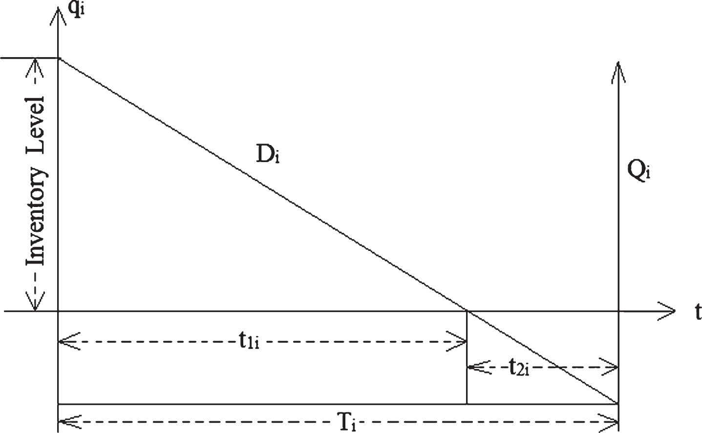
t_1i = the length of time interval in which the inventory level drops to zero

t_2i = the length of time interval in which the inventory reach negative

T_i = length of the inventory per cycle for the ith item, here T_i = t_1i + t_2i

B = budget available for replenishment, ${\tilde{B}}^{I}$ being the generalized intuitionistic fuzzy variable

F = available storage space in the inventory system, ${\tilde{F}}^{I}$ being the generalized intuitionistic fuzzy variable

t = transpose of the matrix.

In addition, the following assumptions are made in developing our mathematical model:

The replenishment rate is infinite and lead time is zero.

Shortages are allowed and completely backlogged.

The deterioration rate of items is constant.

The demand rate D_i (t) is a deterministic function of the stock level; that is: $\begin{matrix} D_{i} (t) \\ = {\begin{matrix} α_{i} + β_{i} q_{i} (t), & if 0 \leq t \leq t_{1 i}, q_{i} (t) \geq 0; \\ \frac{α_{i} + δ_{2 i} q_{i} (t)}{1 + δ_{1 i} (T_{i} - t)}, & if t_{1 i} < t \leq T_{i}, q_{i} (t) > 0; \end{matrix} \end{matrix}$ where, α_i, β_i, δ_1i and δ_2i are positive constants (0 < δ_1i ≤ 1, 0 < δ_2i ≤ 1).

Holding cost per unit per unit time is purchasing price dependent, i.e, $h_{i} = γ_{i} c_{i} 0 < γ_{i} < 1 .$

5 Mathematical formulation of the inventory problem

Using the above notations and assumptions, the inventory model depicted in Fig. 2. Here, the inventory occurs due to combined effects of demand and deterioration in the interval (0, t_1i] and the inventory level reaches zero at t = t_1i, and the demand backlogged in the interval (t_1i, T_i]. Hence, the differential equations representing the inventory level given by:

Fig. 2

Graphical representation of multi-item inventory systems.

$\frac{{dq}_{i} (t)}{dt} = {\begin{matrix} - α_{i} - β_{i} q_{i} (t) & 0 \leq t \leq t_{1 i} \\ - \frac{α_{i} + δ_{2 i} q_{i} (t)}{1 + δ_{1 i} (T_{i} - t)} & t_{1 i} < t \leq T_{i} \end{matrix}$ (33)

From (30), if 0 ≤ t ≤ t_1i, then $\frac{{dq}_{i} (t)}{dt} = - α_{i} - β_{i} q_{i} (t)$

By q_i (t_1i) =0, we have $q_{i} (t) = \frac{α_{i}}{β_{i} + ɛ_{i}} [e^{(β_{i} + ɛ_{i}) (t_{1 i} - t)} - 1]$ (34)

Further, if t_1i < t ≤ T_i, then $\frac{{dq}_{i} (t)}{dt} = - \frac{α_{i} + δ_{2 i} q_{i} (t)}{1 + δ_{1 i} (T_{i} - t)}$

So, we have $q_{i} (t) = - \frac{α_{i}}{δ_{2 i}} [1 - {(\frac{1 + δ_{1 i} (T_{i} - t)}{1 + δ_{1 i} (T_{i} - t_{1 i})})}^{\frac{δ_{2 i}}{δ_{1 i}}}]$ (35)

The ordering quantity over the replenishment cycle for the ith item can be determined as

$\begin{matrix} Q_{i} & = & q_{i} (0) - q_{i} (T_{i}) \\ = & \frac{α_{i} (e^{(β_{i} + ɛ_{i}) t_{1 i}} - 1)}{β_{i} + ɛ_{i}} \\ + \frac{α_{i}}{δ_{2 i}} {1 - {[1 + δ_{1 i} (T_{i} - t_{1 i})]}^{- \frac{δ_{2 i}}{δ_{1 i}}}} \end{matrix}$ (36)

Now we are calculate the different type of cost for the ith item (i = 1, 2, …, n), which are based on previous Equations (33), (34) and (35).

The ordering cost per cycle for ith item is A_i.

Holding cost of the ith item is given by

$\begin{matrix} = & h_{i} \int_{0}^{t_{1 i}} q_{i} (t) dt \\ = & γ_{i} c_{i} \int_{0}^{t_{1 i}} \frac{α_{i}}{β_{i} + ɛ_{i}} [e^{(β_{i} + ɛ_{i}) (t_{1 i} - t)} - 1] dt \\ = & \frac{γ_{i} c_{i} α_{i}}{(β_{i} + ɛ_{i})^{2}} [e^{(β_{i} + ɛ_{i}) t_{1 i}} - 1 - (β_{i} + ɛ_{i}) t_{1 i}] \end{matrix}$ (37)

Sales revenue cost for the ith item is

$\begin{matrix} = & S_{i} \int_{0}^{T_{i}} D_{i} (t) dt \\ = & S_{i} \int_{0}^{t_{1 i}} (α_{i} + β_{i} q_{i} (t)) dt \\ + S_{i} \int_{t_{1 i}}^{T_{i}} \frac{α_{i} + δ_{2 i} q_{i} (t)}{1 + δ_{1 i} (T_{i} - t_{1 i})} dt \\ = & \frac{S_{i} β_{i} α_{i}}{(β_{i} + ɛ_{i})^{2}} [e^{(β_{i} + ɛ_{i}) t_{1 i}} - 1 - (β_{i} + ɛ_{i}) t_{1 i}] \\ - \frac{S_{i} α_{i}}{δ_{2 i}} {[1 + δ_{i} (T_{i} - t_{1 i})]}^{- \frac{δ_{2 i}}{δ_{1 i}}} \\ + \frac{S_{i} α_{i}}{δ_{2 i}} + S_{i} α_{i} t_{1 i} \end{matrix}$ (38)

Purchase cost of the ith the item is given by

$\begin{matrix} = & c_{i} (q_{i} (0) - q_{i} (T_{i})) \\ = & \frac{α_{i} c_{i}}{β_{i} + ɛ_{i}} [e^{(β_{i} + ɛ_{i}) t_{1 i}} - 1] \\ + \frac{α_{i} c_{i}}{δ_{2 i}} {1 - {[1 + δ_{1 i} (T_{i} - t_{1 i})]}^{- \frac{δ_{2 i}}{δ_{1 i}}}} \end{matrix}$ (39)

Opportunity cost of the ith item is given by

$\begin{matrix} = & R_{i} \int_{t_{1 i}}^{T_{i}} (α_{i} - \frac{α_{i} + δ_{2 i} q_{i} (t)}{1 + δ_{1 i} (T_{i} - t)}) dt \\ = & α_{i} R_{i} (T_{i} - t_{1 i}) \\ + \frac{R_{i} α_{i}}{δ_{2 i}} {{[1 + δ_{1 i} (T - t_{1 i})]}^{- \frac{δ_{2 i}}{δ_{1 i}}} - 1} \end{matrix}$ (40)

Shortage cost for the ith item is given by

$\begin{matrix} = & c_{2 i} \int_{t_{1 i}}^{T_{i}} q_{i} (t) dt \\ = & \frac{c_{2 i} α_{i}}{δ_{2 i}} \int_{t_{1 i}}^{T_{i}} (1 - {[\frac{1 + δ_{1 i} (T_{i} - t)}{1 + δ_{1 i} (T_{i} - t_{1 i})}]}^{- \frac{δ_{2 i}}{δ_{1 i}}}) dt \\ = & \frac{c_{2 i} α_{i}}{δ_{2 i}} (T_{i} - t_{1 i}) + \frac{c_{2 i} α_{i}}{δ_{2 i} (δ_{1 i} + δ_{2 i})} \\ {{[1 + δ_{1 i} (T_{i} - t_{1 i})]}^{- \frac{δ_{2 i}}{δ_{1 i}}} - [1 + δ_{1 i} (T_{i} - t_{1 i})]} \end{matrix}$ (41)

Therefore, the total average profit per unit time of our problem is

$\begin{matrix} TP (t_{1 i}, T_{i}) \\ = \frac{1}{T_{i}} [salesrevenue - holdingcost \\ - orderingcost - shortagecost \\ - opportunitycost - purchasingcost] \end{matrix}$

$\begin{matrix} TP (t_{1}, T) \\ = \sum_{i = 1}^{n} \frac{α_{i}}{T_{i}} [\frac{β_{i} S_{i} - γ_{i} c_{i} - (β_{i} + ɛ_{i}) c_{i}}{(β_{i} + ɛ_{i})^{2}} \\ {e^{(β_{i} + ɛ_{i}) t_{1 i}} - 1 - (β_{i} + ɛ_{i}) t_{1 i}} + \frac{(S_{i} - c_{i}) t_{1 i}}{δ_{2 i}} \\ {1 - [1 + δ_{1 i} (T_{i} - t_{1 i})]^{- \frac{δ_{2 i}}{δ_{1 i}}} + δ_{2 i} t_{1 i}} \\ - \frac{c_{2 i} + R_{i} (δ_{1 i} + δ_{2 i})}{(δ_{1 i} + δ_{2 i}) δ_{2 i}} {δ_{2 i} (T - t_{1 i}) \\ + [1 + δ_{1 i} (T_{i} - t_{1 i})]^{- \frac{δ_{2 i}}{δ_{1 i}}} - 1} - A_{i}] \end{matrix}$ (42)

Our problem is to maximize the total average profit under two constraints, such as one budget constraints and another space constraints. Hence, the multi-item crisp inventory problem is given by

$\begin{matrix} Max TP (t_{1}, T) & = & Max \sum_{i = 1}^{n} \frac{α_{i}}{T_{i}} [\frac{β_{i} S_{i} - γ_{i} c_{i} - (β_{i} + ɛ_{i}) c_{i}}{(β_{i} + ɛ_{i})^{2}} {e^{(β_{i} + ɛ_{i}) t_{1 i}} - 1 - (β_{i} + ɛ_{i}) t_{1 i}} \\ + \frac{(S_{i} - c_{i}) t_{1 i}}{δ_{2 i}} {1 - [1 + δ_{1 i} (T_{i} - t_{1 i})]^{- \frac{δ_{2 i}}{δ_{1 i}}} + δ_{2 i} t_{1 i}} \\ - \frac{c_{2 i} + R_{i} (δ_{1 i} + δ_{2 i})}{(δ_{1 i} + δ_{2 i}) δ_{2 i}} {δ_{2 i} (T - t_{1 i}) + [1 + δ_{1 i} (T_{i} - t_{1 i})]^{- \frac{δ_{2 i}}{δ_{1 i}}} - 1} - A_{i}] \\ subject to & \sum_{i = 1}^{n} c_{i} [\frac{α_{i} (e^{(β_{i} + ɛ_{i}) t_{1 i}} - 1)}{β_{i} + ɛ_{i}} + \frac{α_{i}}{δ_{2 i}} {1 - {[1 + δ_{1 i} (T_{i} - t_{1 i})]}^{- \frac{δ_{2 i}}{δ_{1 i}}}}] \leq B; \end{matrix}$ (43) $\begin{matrix} \sum_{i = 1}^{n} w_{i} [\frac{α_{i} (e^{(β_{i} + ɛ_{i}) t_{1 i}} - 1)}{β_{i} + ɛ_{i}} + \frac{α_{i}}{δ_{2 i}} {1 - {[1 + δ_{1 i} (T_{i} - t_{1 i})]}^{- \frac{δ_{2 i}}{δ_{1 i}}}}] \leq F; \\ t_{1} \geq 0, T \geq 0 \end{matrix}$ where t₁ = (t₁₁, t₁₂, …, t_1n) ^t and T = (T₁, T₂, …, T_n) ^t are decision variables.

When the inventory costs c_i, c_2i, R_i, A_i, selling price S_i, storage space w_i, total budget B_i and total available space F_i become generalized intuitionistic fuzzy variables, the present multi-item generalized intuitionistic fuzzy inventory model is of theform:

$\begin{matrix} Max {\tilde{TP}}^{I} (t_{1}, T) & = & Max \sum_{i = 1}^{n} \frac{α_{i}}{T_{i}} [\frac{β_{i} {\tilde{S}}_{i}^{I} - γ_{i} {\tilde{c}}_{i}^{I} - (β_{i} + ɛ_{i}) {\tilde{c}}_{i}^{I}}{(β_{i} + ɛ_{i})^{2}} {e^{(β_{i} + ɛ_{i}) t_{1 i}} - 1 - (β_{i} + ɛ_{i}) t_{1 i}} \\ + \frac{({\tilde{S}}_{i}^{I} - {\tilde{c}}_{i}^{I}) t_{1 i}}{δ_{2 i}} {1 - [1 + δ_{1 i} (T_{i} - t_{1 i})]^{- \frac{δ_{2 i}}{δ_{1 i}}} + δ_{2 i} t_{1 i}} \\ - \frac{{\tilde{c}}_{2 i}^{I} + {\tilde{R}}_{i}^{I} (δ_{1 i} + δ_{2 i})}{(δ_{1 i} + δ_{2 i}) δ_{2 i}} {δ_{2 i} (T - t_{1 i}) + [1 + δ_{1 i} (T_{i} - t_{1 i})]^{- \frac{δ_{2 i}}{δ_{1 i}}} - 1} - {\tilde{A}}_{i}^{I}] \\ subject to & {\tilde{g}}_{1}^{I} (t_{1}, T) = \sum_{i = 1}^{n} {\tilde{c}}_{i}^{I} [\frac{α_{i} (e^{(β_{i} + ɛ_{i}) t_{1 i}} - 1)}{β_{i} + ɛ_{i}} + \frac{α_{i}}{δ_{2 i}} {1 - {[1 + δ_{1 i} (T_{i} - t_{1 i})]}^{- \frac{δ_{2 i}}{δ_{1 i}}}}] \leq {\tilde{B}}^{I}; \\ {\tilde{g}}_{2}^{I} (t_{1}, T) = \sum_{i = 1}^{n} {\tilde{w}}_{i}^{I} [\frac{α_{i} (e^{(β_{i} + ɛ_{i}) t_{1 i}} - 1)}{β_{i} + ɛ_{i}} + \frac{α_{i}}{δ_{2 i}} {1 - {[1 + δ_{1 i} (T_{i} - t_{1 i})]}^{- \frac{δ_{2 i}}{δ_{1 i}}}}] \leq {\tilde{F}}^{I}; \\ t_{1} \geq 0, T \geq 0 \end{matrix}$ (44) where t₁ = (t₁₁, t₁₂, …, t_1n) ^t and T = (T₁, T₂, …, T_n) ^t are decision variables.

Or, $\begin{matrix} Z & = & Max {\tilde{TP}}^{I} (t_{1}, T) \\ subject to & {\tilde{g}}_{1}^{I} (t_{1}, T) \leq {\tilde{B}}^{I}; \end{matrix}$ (45) $\begin{matrix} {\tilde{g}}_{2}^{I} (t_{1}, T) \leq {\tilde{F}}^{I}; \\ t_{1} \geq 0, T \geq 0 \end{matrix}$ where t₁ = (t₁₁, t₁₂, …, t_1n) ^t and T = (T₁, T₂, …, T_n) ^t are decision variables.

5.1 Solution methodology

To solve the multi-items generalized intuitionistic fuzzy inventory problem (Equation 45) is based on possibility mean and possibility variance. Then we have proposed the following methods.

Method-I: We transform the multi-items generalized intuitionistic fuzzy inventory problem (45) into the deterministic problem under the possibility mean. Thus we have the following deterministic multi-items inventory problem. $\begin{matrix} Z_{1} & = & Max M [{\tilde{TP}}^{I} (t_{1}, T)] \\ subject to & M [{\tilde{g}}_{1}^{I} (t_{1}, T) \leq {\tilde{B}}^{I}]; \end{matrix}$ (46) $\begin{matrix} M [{\tilde{g}}_{2}^{I} (t_{1}, T) \leq {\tilde{F}}^{I}]; \\ t_{1} \geq 0, T \geq 0 \end{matrix}$ where t₁ = (t₁₁, t₁₂, …, t_1n) ^t and T = (T₁, T₂, …, T_n) ^t are decision variables.

Method-II: We transform the multi-items generalized intuitionistic fuzzy inventory problem (45) into the deterministic problem through the possibility variance. Thus we have the following deterministic multi-items inventory problem. $\begin{matrix} Z_{2} & = & Max V [{\tilde{TP}}^{I} (t_{1}, T)] \\ subject to & V [{\tilde{g}}_{1}^{I} (t_{1}, T) \leq {\tilde{B}}^{I}]; \end{matrix}$ (47) $\begin{matrix} V [{\tilde{g}}_{2}^{I} (t_{1}, T) \leq {\tilde{F}}^{I}]; \\ t_{1} \geq 0, T \geq 0 \end{matrix}$ where t₁ = (t₁₁, t₁₂, …, t_1n) ^t and T = (T₁, T₂, …, T_n) ^t are decision variables.

6 Numerical example

A manufacturing company produces some items and stock these items in a warehouse. The company has a warehouse whose total floor area (F) = (2500, 3000, 3500, 4500 ; 0.6) (2000, 3000, 3500, 5000 ; 0.4) m² and total available budget (B) = $ (4000, 5500, 5750, 7500 ; 0.6) (3500, 5500, 5750, 8000 ; 0.4). The costs of these inventory problem are given in Table-2 and input crisp parameters are given in Table-1. Find out optimal length of the inventory (T_i), length of the non-negative inventory (t_1i), optimal order quantity (Q_i) and total average profit (TP).

Table 1
Input crisp parameters

Item α _i β _i δ _1i δ _2i

I 650 0.35 0.7 0.3

II 600 0.45 0.6 0.4

Item	α _i	β _i	δ _1i	δ _2i
I	650	0.35	0.7	0.3
II	600	0.45	0.6	0.4

Table 2

Input generalized intuitionistic fuzzy parameters

Item	I	II
${\tilde{c}}_{i}^{I}$	$(6.0,7.00,9.00,11; 0.6)(4.0,7.00,9.00,12; 0.4)	$(5.0,6.00,9.00,10; 0.6)(3.0, 6.00,9.00,11; 0.4)
${\tilde{c}}_{2 i}^{I}$	$(3.0,4.00,6.00,7.0;0.6)(2.0,4.00,6.00,9.0;0.4)	$(2.0,3.00,4.00,5.0;0.6)(1.0, 3.00,4.00,6.0;0.4)
${\tilde{w}}_{i}^{I}$	(1.5,2.00,2.50,4.0;0.6)(0.5,2.0,2.50,5.50;0.4)m²	(2.0,2.50,3.50,4.0;0.6)(1.0, 2.50,3.50,5.0;0.4)m²
${\tilde{R}}_{i}^{I}$	$(6.0,8.00,9.00,10; 0.6)(4.0,8.00,9.00,12; 0.4)	$(7.0,9.00,11.0,12; 0.6)(6.0, 9.00,11.0,14; 0.4)
${\tilde{S}}_{i}^{I}$	$(9.0,11.0,13.0,14; 0.6)(6.0,11.0,13.0,15; 0.4)	$(8.0,10.0,12.0,13; 0.6)(5.0,10.0,12.0,14; 0.4)
${\tilde{A}}_{i}^{I}$	$(300,400,420,560; 0.6)(260,400,420,600;0.4)	$(310,420,482,580;0.6)(280,420,482,620; 0.4)

The above problem can be solved by two different proposed methods as Method-I & Method-II. Method-I give different optimal solutions for different values of ɛ_i & γ_i as shown in Tables-3 and 4 respectively. Similarly, Method-II gives different optimal solutions for different values of ɛ_i & γ_i as shown in Tables-5 and 6 respectively.

Table 3

Optimal solutions (Method-I) for fixed value of γ₁ = 0.5, γ₂ = 0.6

Item	ɛ _i	t _1i	t _2i	T _i	Q _i	Z ₁
I	0.02	0.5396	0.1245	0.6641	464.445	906.915
II	0.03	0.5666	0.1475	0.7141	473.143
I	0.03	0.5309	0.1260	0.6569	459.506	891.814
II	0.04	0.5584	0.1490	0.7075	468.653
I	0.04	0.5226	0.1275	0.6501	454.761	877.001
II	0.05	0.5505	0.1506	0.7011	464.322
I	0.05	0.5145	0.1289	0.6435	450.199	862.465
II	0.06	0.5428	0.1521	0.6950	460.141
I	0.06	0.5068	0.1304	0.6372	445.808	848.199
II	0.07	0.5354	0.1536	0.6834	456.101
I	0.07	0.4993	0.1318	0.6312	441.578	834.199
II	0.08	0.5282	0.1551	0.6834	452.195
I	0.08	0.4921	0.1332	0.6253	437.499	820.436
II	0.09	0.5212	0.1566	0.6779	448.417

Table 4

Optimal solutions (Method-I) for fixed value of ɛ₁ = 0.04, ɛ₂ = 0.05

Item	γ _i	t _1i	t _2i	T _i	Q _i	Z ₁
I	0.45	0.5622	0.1203	0.6825	482.446	984.831
II	0.50	0.6304	0.1351	0.7656	520.708
I	0.50	0.5226	0.1275	0.6501	454.761	909.963
II	0.55	0.5870	0.1432	0.7303	489.612
I	0.55	0.4893	0.1341	0.6234	432.175	842.116
II	0.60	0.5505	0.1506	0.7011	464.322
I	0.60	0.4608	0.1401	0.6010	413.339	780.147
II	0.65	0.5191	0.1574	0.6760	443.282
I	0.65	0.4360	0.1458	0.5818	397.353	723.183
II	0.70	0.4918	0.1638	0.6556	425.461
I	0.70	0.4142	0.1510	0.5653	383.589	670.542
II	0.75	0.4678	0.1697	0.6375	410.142

Table 5

Optimal solutions (Method-II) for fixed value of γ₁ = 0.5, γ₂ = 0.6

Item	ɛ _i	t _1i	t _2i	T _i	Q _i	Z ₂
I	0.02	0.7696	0.4466	1.2196	681.095	739.011
II	0.03	0.4896	0.2813	0.7711	479.404
I	0.03	0.7729	0.4394	1.2117	677.209	734.142
II	0.04	0.4845	0.2830	0.7675	477.115
I	0.04	0.7748	0.4324	1.2073	673.443	729.365
II	0.05	0.4795	0.2846	0.7642	474.875
I	0.05	0.7774	0.4257	1.2031	669.791	724.677
II	0.06	0.4746	0.2863	0.7610	472.683
I	0.06	0.7798	0.4191	1.1990	666.249	720.076
II	0.07	0.4698	0.2879	0.7578	470.539
I	0.07	0.7822	0.4128	1.1950	662.810	715.558
II	0.08	0.4651	0.2895	0.7546	468.439
I	0.08	0.7845	0.4066	1.1912	659.472	711.122
II	0.09	0.4605	0.2910	0.7516	466.383

Table 6

Optimal solutions (Method-II) for fixed value of ɛ₁ = 0.04, ɛ₂ = 0.05

Item	γ _i	t _1i	t _2i	T _i	Q _i	Z ₂
I	0.45	0.7621	0.4653	1.2274	694.405	768.169
II	0.50	0.5251	0.2690	0.7942	502.764
I	0.50	0.7748	0.4324	1.2073	673.443	744.608
II	0.55	0.5011	0.2771	0.7783	487.942
I	0.55	0.7860	0.4040	1.1901	655.612	723.107
II	0.60	0.4795	0.2846	0.7642	474.875
I	0.60	0.7958	0.3793	1.1751	640.247	703.379
II	0.65	0.4599	0.2917	0.7517	463.258
I	0.65	0.8045	0.3574	1.2274	626.802	685.191
II	0.70	0.4420	0.2984	0.7405	452.857
I	0.70	0.8123	0.3380	1.2274	615.091	668.353
II	0.75	0.4256	0.3047	0.7304	443.485

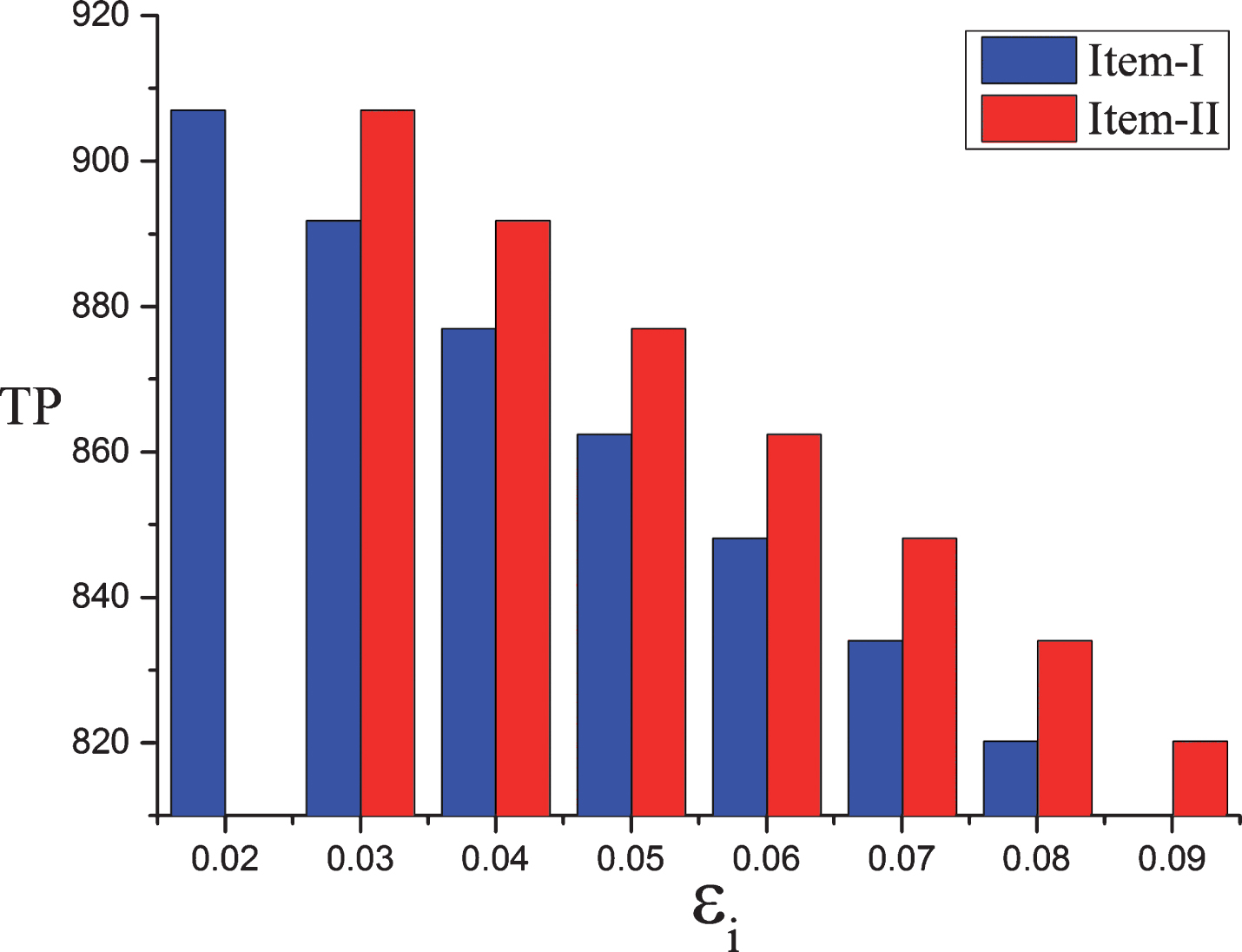
As shown in Tables-3 and 5, if ɛ_i increasing, the length of the non-negative inventory (t_1i) and ordering cycle (T) will decrease, but the length of shortage period (t_2i) will increase. The optimal profit (TP) and ordering quantity (Q_i) are also decreasing in ɛ_i. In this case, the seller will increase the ordering frequency and shorten the ordering cycle.

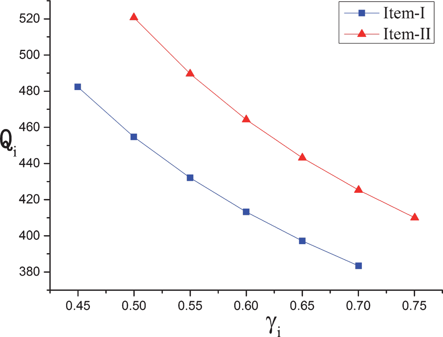
Further, from Tables-4 and 6 we can see that if γ_i is increasing, the length of shortage period (t_2i) will increase, but the length of time interval with non-negative inventory (t_1i) and ordering cycle (T) will decrease. As same γ_i the optimal profit (TP) and ordering quantity (Q_i) are also decreasing. From the computing results, optimal order quantity (Q_i), ordering cycle (T) and total profit (TP) are effected as very higher deterioration (ɛ_i). As ɛ_i increasing, the length of shortage period (t_2i) is very high. In this case, many people are willing to accept the back order, so the sellers have no loser by extending the length of shortage period.

6.1 Comparison analysis with the Chakraborty et al. method based on IFN expected value

If we consider GTIFNs parameters, i.e., ${\tilde{c}}_{i}^{I}$ , ${\tilde{c}}_{2 i}^{I}$ , ${\tilde{w}}_{i}^{I}$ , ${\tilde{R}}_{i}^{I}$ , ${\tilde{S}}_{i}^{I}$ , ${\tilde{A}}_{i}^{I}$ , ${\tilde{B}}^{I}$ , ${\tilde{F}}^{I}$ as IFNs parameters, then the generalized intuitionistic fuzzy inventory problem (44) will transform to the intuitionistic fuzzy inventory problem. The input value of intuitionistic fuzzy parameters ${\tilde{c}}_{i}^{IN}$ , ${\tilde{c}}_{2 i}^{IN}$ , ${\tilde{w}}_{i}^{IN}$ , ${\tilde{R}}_{i}^{IN}$ , ${\tilde{S}}_{i}^{IN}$ , ${\tilde{A}}_{i}^{IN}$ , ${\tilde{B}}^{IN}$ , ${\tilde{F}}^{IN}$ of the proposed inventory problem are given in Table-7. A comparative analysis is presented between proposed methodology and methodology proposed by Chakraborty et al. [32]. Using [32], we have solved intuitionistic fuzzy inventory problem (44) and the optimize results are shown in Table-8. From Tables-3 and 8, it is clearly visible that if retailer’s adopt the proposed methodology then it will be beneficial. In addition, Table-9 described the optimal results of problem (44) with different weighted values.

Table 7
Input intuitionistic fuzzy parameters

Item I II

${\tilde{c}}_{i}^{IN}$ $(6.0,7.00,9.00,11)(4.0,7.00,9.00,12) $(5.0,6.00,9.00,10)(3.0, 6.00,9.00,11)

${\tilde{c}}_{2 i}^{IN}$ $(3.0,4.00,6.00,7.0)(2.0,4.00,6.00,9.0) $(2.0,3.00,4.00,5.0)(1.0, 3.00,4.00,6.0)

${\tilde{w}}_{i}^{IN}$ (1.5,2.00,2.50,4.0)(0.5,2.0,2.50,5.50)m² (2.0,2.50,3.50,4.0)(1.0, 2.50,3.50,5.0)m²

${\tilde{R}}_{i}^{IN}$ $(6.0,8.00,9.00,10)(4.0,8.00,9.00,12) $(7.0,9.00,11.0,12)(6.0, 9.00,11.0,14)

${\tilde{S}}_{i}^{IN}$ $(9.0,11.0,13.0,14)(6.0,11.0,13.0,15) $(8.0,10.0,12.0,13)(5.0,10.0,12.0,14)

${\tilde{A}}_{i}^{IN}$ $(300,400,420,560)(260,400,420,600) $(310,420,482,580)(280,420,482,620)

Item	I	II
${\tilde{c}}_{i}^{IN}$	$(6.0,7.00,9.00,11)(4.0,7.00,9.00,12)	$(5.0,6.00,9.00,10)(3.0, 6.00,9.00,11)
${\tilde{c}}_{2 i}^{IN}$	$(3.0,4.00,6.00,7.0)(2.0,4.00,6.00,9.0)	$(2.0,3.00,4.00,5.0)(1.0, 3.00,4.00,6.0)
${\tilde{w}}_{i}^{IN}$	(1.5,2.00,2.50,4.0)(0.5,2.0,2.50,5.50)m²	(2.0,2.50,3.50,4.0)(1.0, 2.50,3.50,5.0)m²
${\tilde{R}}_{i}^{IN}$	$(6.0,8.00,9.00,10)(4.0,8.00,9.00,12)	$(7.0,9.00,11.0,12)(6.0, 9.00,11.0,14)
${\tilde{S}}_{i}^{IN}$	$(9.0,11.0,13.0,14)(6.0,11.0,13.0,15)	$(8.0,10.0,12.0,13)(5.0,10.0,12.0,14)
${\tilde{A}}_{i}^{IN}$	$(300,400,420,560)(260,400,420,600)	$(310,420,482,580)(280,420,482,620)

Table 8

Optimal solutions (by Chakraborty et al. [32] method) for fixed value of γ₁ = 0.5, γ₂ = 0.6

Item	ɛ _i	t _1i	t _2i	T _i	Q _i	Z ₁
I	0.02	0.2547	0.1802	0.4349	281.162	798.367
II	0.03	0.3353	0.1809	0.5174	318.491
I	0.03	0.2499	0.1809	0.4309	278.400	784.240
II	0.04	0.3284	0.1830	0.5115	314.525
I	0.04	0.2453	0.1817	0.4270	275.752	770.519
II	0.05	0.3218	0.1841	0.5059	310.748
I	0.05	0.2409	0.1824	0.4234	273.212	757.169
II	0.06	0.3155	0.1850	0.5006	307.146
I	0.06	0.2367	0.1831	0.4199	270.772	744.189
II	0.07	0.3095	0.1860	0.4956	303.708
I	0.07	0.2326	0.1838	0.4165	268.427	731.556
II	0.08	0.3037	0.1869	0.4907	300.420

Table 9

Optimal Solution(Method-I) for Different Weighted Value

$w_{\tilde{a}}$	$u_{\tilde{a}}$	Max TP
0.6	0.4	906.9150
0.7	0.3	956.4150
0.8	0.2	985.5010
0.9	0.1	1005.132
1	0.0	1032.884

7 Discussion

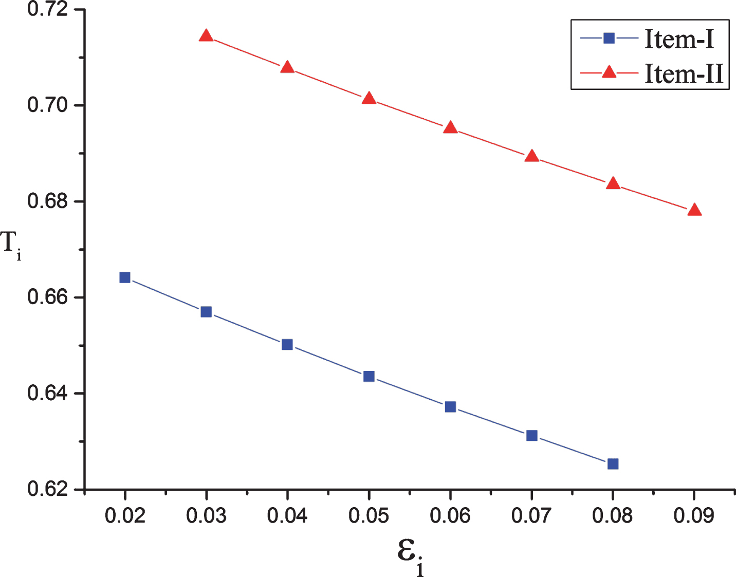
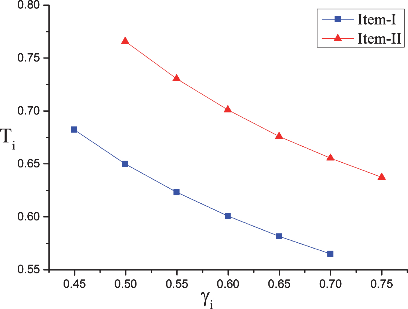
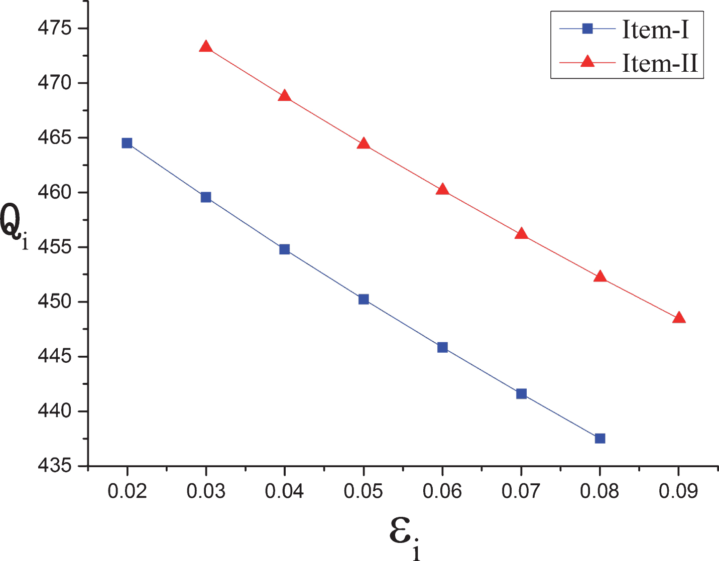
Based on the solutions obtained in Tables-3– 6, and 9 we can say that manufacturing company keep in mind maximum profit gained for certain values of purchasing cost coefficient (γ), when deterioration is fixed. Here, the manufacturing company try to invest huge amount as far as possible in order to ensure the maximum profit, but anyhow it should not exceed the production cost of absolute demand quantity. For slight deterioration of the products, we suggested that manufacturing company to fixed γ. In this case, we have seen company will earn better profit. Therefore, from the Tables 3–6, and 9 following observations can be constructed. These are also depicted in Figs. 3–8.

Fig. 3

ɛ_i Vs. T_i.

Fig. 4

γ_i Vs. T_i.

Fig. 5

ɛ_i Vs. Q_i.

Fig. 6

γ_i Vs. Q_i.

Fig. 7

ɛ_i Vs. TP.

Fig. 8

γ_i Vs. TP.

Increasing the both deterioration rate ɛ_i and parameter γ_i, then the time length of total inventory T_i decreases (cf. Figs. 1 and 4).

The ordering quantity Q_i of the inventory system decreases with the increase of both parameter γ_i and deterioration rate ɛ_i (cf. Figs. 5 and 6).

The total average profit TP of the inventory problem decreases with the increase of both deterioration rate ɛ_i and parameter γ_i (cf. Figs. 7 and 8).

The total average profit TP of the proposed inventory problem is increases when degrees of both membership value $w_{\tilde{a}}$ increase and non-membership value $u_{\tilde{a}}$ decrease for all the generalized intuitionistic fuzzy parameters.

8 Conclusion

As an eminent issue of IFSs, GIFNs are the consistent tools to fleet the fuzzy and uncertain quantities with hesitance degrees. The notion of a GIFNs are of great importance in fuzzy optimization. For the first time the mathematical representation of possibility mean, variance and covariance in GTIFNs environment has carried out in this paper. We have formulated a MGIFim with inventory level dependent demand. In this model the holding cost is considered as a function of purchasing price and backlogging is permitted. Possibility mean and variance technique (Method-I and Method-II) are exercised to solve multi-item generalized intuitionistic fuzzy inventory problem. In Tables-3 and 4, we have shown the optimal solutions of problem (46) for different values of ɛ_i & γ_i respectively. In Tables-5 and 6, we have shown the optimal solutions of problem (47) for different values of ɛ_i & γ_i respectively.

For future researches in this area, the followings are recommended:

Possibility mean, variance and covariance of other intuitionistic fuzzy numbers can be formulated.

The Possibility mean and variance of GTIFN can be employed in MADM problems.

In the proposed model, quantity discounts can be allowed. In addition to back orders, lost sales can also be assumed for shortages.

The present methodology can be applied to three layer supply chain model considering inflation, variable deterioration, stock-dependent holding cost, etc.

Possibility mean, variance and covariance oftype-2 intuitionistic fuzzy number can not trace out in this way. The proposed methodology not applicable for large non-linear inventory problems. These are the limitation of the proposed methodology.

References

Zadeh

L.A.

, Fuzzy sets, Information and Control 8 (1965), 338–356.

Atanassov

T.K.

, Intuitionistic fuzzy sets, Fuzzy Sets and System 20 (1986), 87–96.

Dubois

, Prade

, Fuzzy Sets and Systems: Theory and Applications Academic Press, New York 1980.

D.F.

, A note on “using intuitionistic fuzzy sets for fault-tree analysis on printed circuit board assembly”, Microelectronics Reliability 48 (2008), 17–41.

Wan

S.P.

, Multi-attribute decision making method based on possibility variance coefficient of triangular intuitionistic fuzzy numbers, International Journal Uncertainty Fuzziness Knowledge Based System 21 (2013), 223–243.

Wan

S.P.

and Dong

J.Y.

, Possibility method for triangular intuitionistic fuzzy multi-attribute group decision making with incomplete weight information, Intentional Journal Computation Intelligent System 7 (2015), 65–79.

Wang

J.Q.

and Zhang

, Aggregation operators on intuitionistic trapezoidal fuzzy number and its application to multi-criteria decision making problems, Journal of System Engineering Electronic 20 (2019), 321–326.

and Liu

Y.J.

, An approach for multiple attribute group decision making problems with interval-valued intuitionistic trapezoidal fuzzy numbers, Computational Industrial Engineering 66 (2013), 311–324.

Zadeh

L.A.

, Fuzzy sets as a basis for a theory of possibility, Fuzzy Sets and System 1 (1978), 3–28.

10.

Dubois

and Prade

, Possibility theory, An approach to computerized processing of uncertainty, Plenum, New York, 1988.

11.

Klir

K.J.

, On fuzzy set interpretation of possibility, Fuzzy Sets and System 108 (1999), 263–273.

12.

Yager

, On the specificity of a possibility distribution, Fuzzy Sets and System 50 (1992), 279–292.

13.

Fuller

and Majlender

, On weighted possibilistic mean and variance of fuzzy numbers, Fuzzy Sets and Systems 136 (2003), 363–374.

14.

Carlsson

and Fuller

, On possibilistic mean value and variance of fuzzy numbers, Fuzzy Sets and System 122 (2001), 315–326.

15.

Wan

S.P.

, Li

D.F.

and Rui

Z.F.

, Possibility mean, variance and covariance of triangular intuitionistic fuzzy numbers, Journal of Intelligent & Fuzzy Systems 24 (2013), 847–858.

16.

Guptaand

and Vrat

, Inventory model with multi-items under constraint systems for stock dependent consumption rate, Operation Research 24 (1986), 41–42.

17.

S.K.

, Ouyang

L.Y.

and Yang

T.C.

, An optimal replenishment policy for non instantaneous deteriorating items with stock-dependent demand and partial backlogging, International Journal of Production & Economics 101 (2006), 369–384.

18.

Padmanabhan

and Vrat

, EOQ models for perishable items under stock dependent selling rate, European Journal Operation Research 86 (1995), 281–292.

19.

Chang

H.J.

and Dye

C.Y.

, An EOQ model for deteriorating items with time varying demand and partial backlogging, Journal of Operation Research Society 50 (1999), 1176–1182.

20.

Chung

C.Y.

and Ouyang

L.Y.

, An EOQ model for perishable items under stock-dependent selling rate and time-dependent partial backlogging, European Journal Operation Research 163 (2005), 776–783.

21.

Chang

C.T.

, Goyal

S.K.

and Teng

J.T.

, On An EOQ model for perishable items under stock-dependent selling rate and timedependent partial backlogging by Dye and Ouyang, European Journal Operation Research 174 (2006), 923–929.

22.

Lee

Y.P.

and Dye

C.Y.

, An inventory model for deteriorating items under stock-dependent demand and controllable deterioration rate, European Journal of Operation Research 63 (2012), 474–482.

23.

Pando

, San-Jose

A.L.

, Garcia-Laguna

and Sicilia

, An economic lot size model with non-linear holding cost hinging on time and quantity, International Journal of Production Economics 145 (2013), 294–303.

24.

Tripathi

P.E.

, Inventory model with different demand rate and different holding cost, International Journal of Industrial Engineering & Computation 4 (2013), 437–446.

25.

Valliathal

and Unthayakumar

, Designing a new computational approach of partial backlogging on the economic production quantity model for deterioration items with non-linear holding cost under inflationary conditions, Optimization Letters 5 (2011), 515–530.

26.

Rani

, Gulati

T.R.

and Garg

, Multi-objective non-linear programming problem in intuitionistic fuzzy environment: Optimistic and pessimistic view point, Expert Systems with Applications 64 (2016), 228–238.

27.

Garg

and Ansha , Arithmetic operations on generalized parabolic fuzzy number and its Applications, Proceeding of the National Academy of Sciences, India Section A: Physical Sciences, Springer 2016.

28.

Garai

, Chakraborty

and Roy

T.K.

, Expected value of exponential fuzzy number and its application to multi-item deterministic inventory model for deteriorating items, Journal of Uncertainty Analysis and Applications 5 (2017), 1–20.

29.

Garg

, A novel approach for analyzing the reliability of series-parallel system using credibility theory and different types of intuitionistic fuzzy numbers, Journal of Brazilian So Ciety of Mechanical Sciences and Engineering 8 (2016), 1021–1035.

30.

Garg

, Fuzzy Inventory model for deteriorating items using different types of lead-time distributions, Intelligent Techniques in Engineering Management 87 (2015), 247–274.

31.

Garg

, Inventory model involving variable lead time, backorder discounts and lost sales using, World Conference on Soft computing in Industrial Application 1 (2014), pp. 1–12.

32.

Chakraborty

, Jana

D.K.

and Roy

T.K.

, Expected value of intuitionistic fuzzy number and its application to solve multiobjective multi-item solid transportation problem for damageable items in intuitionistic fuzzy environment, Journal of Intelligent & Fuzzy Systems 30 (2016), 1109–1122.

33.

Z.S.

and Yager

R.R.

, Some geometric aggregation operators based on intuitionistic fuzzy sets, International Journal of General Systems 35 (2006), 417–433.

34.

Park

J.H.

, Park

and Lim

K.M.

, Correlation coefficient of generalized intuitionistic fuzzy sets by statistical method, Honam Mathematical Journal 28 (2006), 317–326.

35.

Panigrahi

and Nanda

, A comparison between intuitionistic fuzzy sets and generalized intuitionistic fuzzy sets, Hacettepe University Bulletin of Natural Sciences & Engineering 2006.

36.

Zhou

and He

J.M.

, Intuitionistic fuzzy geometric Bonferroni means and their application in multi-criteria decision making, International Journal of Intelligent Systems 27 (2012), 995–1019.

37.

Zhao

, Xu

, Ni

and Liu

, Generalized aggregation operators for intuitionistic fuzzy sets, 25 (2010), 1–30.

38.

Zhou

, Xu

and Chen

, Preference relations based on hesitant-intuitionistic fuzzy information and their application in group decision making, Computers & Industrial Engineering 87 (2015), 163–175.

39.

Dejian

and Huchang

, Visualization and quantitative research on intuitionistic fuzzy studies, Journal of Intelligent & Fuzzy Systems 30 (2016), 3653–3663.

40.

and Shi

, Researching the development of Atanassov intuitionistic fuzzy set: Using a citation network analysis, Applied Soft Computing 32 (2015), 189–198.

A multi-item generalized intuitionistic fuzzy inventory model with inventory level dependent demand using possibility mean,variance and covariance

Abstract

Keywords

1 Introduction

2 Basic preliminaries

5 Mathematical formulation of the inventory problem

Table 1 Input crisp parameters Item α i β i δ 1i δ 2i I 650 0.35 0.7 0.3 II 600 0.45 0.6 0.4

References

Table 1
Input crisp parameters

Item α _i β _i δ _1i δ _2i

I 650 0.35 0.7 0.3

II 600 0.45 0.6 0.4