Numerical solution of a singularly perturbed problem with Robin boundary conditions using particle swarm optimization algorithm

Abstract

In this paper, a numerical method on a Shishkin mesh to solve the singularly perturbed reaction-diffusion problem with Robin boundary conditions is considered. Especially, for the Robin boundary conditions, a high precision discrete scheme is developed. Then, we first transform the Shishkin mesh transition parameter selection problem into a nonlinear unconstrained optimization problem which is solved by using the basic particle swarm optimization (PSO) algorithm. The experimental results show that the accuracy of numerical solution to singularly perturbed problem on the boundary layers is improved by using the PSO algorithm to optimize Shishkin mesh parameters. It further verifies the feasibility and effectiveness of the proposed method.

Keywords

Singularly perturbed Robin boundary conditions particle swarm optimization Shishkin mesh parameter inversion

1 Introduction

It is well known that singularly perturbed two-points boundary value problems are used to describe the transport processes involving fluid motion, heat transfer, astrophysics, oceanography, meteorology, pollutant and sediment transport, and chemical reactor et al. [1]. Such problems contain one or more perturbation parameters, which can reflect the physical character of the equations. The solution of these problems has a multi-scale character. It has two components, one changes slowly and the other changes quickly. Many standard numerical methods applied to these problems, such as (1) below, may yield inaccurate results. Therefore, in order to obtain a reliable numerical solution, one important approach is the use of suitable layer-adapted meshes that are very fine where layers appear in the solution. In recently years, there has been tremendous interest in developing layer-adapted mesh method to solve the following linear reaction-diffusion problem with Dirichlet boundary conditions $\begin{matrix} - ɛ u^{″} (x) + b (x) u (x) = f (x), \\ x \in Ω = (0, 1), \\ u (0) = u (1) = 0, \end{matrix}$ (1) where b (x) and f (x) are sufficiently smooth functions, and 0 < ɛ ⪡ 1 is a parameter. Specifically, Linß [2] used finite element method to solve the problem (1) on a Shishkin mesh. Cai et al. [3] presented a non-equidistant finite difference method according to the property of boundary layer. Kummar [4] gave a new piecewise uniform mesh of Shishkin type, and used the high order compact finite difference scheme to solve the above problem (1) on this type of mesh. Linß et al. [5] proposed a quadratic C¹ splines collocation method on a modified Shishkin mesh for the above singularly perturbed problem (1). Vulanović [6] considered a modification of the Shishkin mesh and designed a numerical solution to solve one-dimensional reaction-diffusion problem.

However, limited work has been done in numerical methods for the singularly perturbed reaction-diffusion equations with Robin boundary conditions. Thus, in this paper, we consider the following singularly perturbed reaction-diffusion problems $\begin{matrix} ℒ u (x) : = - ɛ u^{″} (x) + b (x) u (x) = f (x), \\ x \in (0, 1) \end{matrix}$ (2) with the Robin boundary conditions, $\begin{matrix} α_{1} u (0) - β_{1} \sqrt{ɛ} u^{'} (0) = γ_{1}, \\ α_{2} u (1) + β_{2} \sqrt{ɛ} u^{'} (1) = γ_{2}, \end{matrix}$ (3) where the parameter 0 < ɛ ⪡ 1 is the singular perturbation parameter. We assume that the functions b (x), f (x) are sufficiently smooth and there exist two positive constants ρ^* and ρ such that $ρ^{*} > b (x) > ρ > 0, x \in [0, 1] .$ (4)

It is also assumed that the coefficients of the conditions (3) satisfy α_k, β_k ≥ 0, α_k + β_k > 0 for k = 1, 2 with $α_{1} \neq β_{1} \sqrt{b (0)}$ . Under condition (4), the problem (2)–(3) has a unique solution, which exhibits sharp boundary layers of width O (ɛ| ln ɛ|) at x = 0 and x = 1. Recently, Natesan et al. [7] developed a parameter uniform numerical method on a Shishkin mesh for these problems, they used a cubic spline function to approximate the derivative boundary conditions.

In conclusion, the Shishkin mesh method is very popular in solving the above singularly perturbed reaction-diffusion equations. This type of mesh contains a grid transition point τ which has some different definitions in some recent papers. In [7], Natesan and Bawa defined τ as follows: $τ = min {\frac{1}{4}, σ_{0} ɛ ln N},$ (5) where σ₀ is a positive parameter. Then, they divided interval [0, 1] into three subintervals, on each of which the mesh is uniform.

As far as we know, in practical computation, most of the authors haven’t given a method to determine the grid parameter σ₀ defined in (5). Therefore, one work of this paper is motivated by the needs for a numerical method to obtain the best mesh transition point. More specifically, we may transform the choice of mesh parameter problem into an unconstrained nonlinear optimization problem. For the complicated nonlinear optimization problem, the traditional optimization methods may not obtain the global optimization efficiently.

Particle swarm optimization (PSO) algorithm is a population-based heuristic global optimization method proposed by Kennedy and Eberhart [13] in 1995. It was first intended for simulating social behaviour, as a stylized representation of the movement of organisms in a bird flock or fish school. PSO can be used to solve multi-objective, non-differentiable problems, and so on. It is very efficient in a lot of research fields such as parameter estimation [15], controller design [14], neural networks [16], image processing [17], signal processing [18]. Very recently, the application of PSO algorithm in the field of numerical analysis has a lot of successful examples: Saidi et al. [19] used PSO algorithm to solve the Schrödinger equation. Lee [20] applied PSO algorithm to the solution of Blasius equation. Pérez et al. [21] presented a discrete PSO algorithm for solving a non-linear Diophantine systems of equations. Babaei [22] introduced a PSO to solve the nonlinear differential equations. Ouyang et al. designed a parallel hybrid PSO algorithm with CUDA for lD heat conduction equation [23], Many others also used evolutionary algorithm to solve differential equations [24, 25].

Another work of this paper is to design a higher accuracy finite difference scheme to discrete the derivative boundary conditions in (3). As far as we know, the derivative boundary conditions in (3) are much more difficult to handle than Dirichlet conditions. We have found that, when the first-order accurate scheme of the derivative boundary conditions is employed, it effects the accuracy of the overall numerical solution even if a second order numerical approach is given at the interior grid points. Recently, some researches [8 –12] considered some differential equations with Neumann boundary conditions, and developed a class of higher accuracy difference schemes to approximate the derivative boundary conditions. In this work, we will use some techniques developed in [10 –12] to study the difference scheme for the Robin boundary conditions (3).

In general, a novel method for the solution of the above problem (2)–(3) based on PSO is introduced. Specifically, based on the finite difference scheme and Shishkin mesh, we first use the double mesh principle to estimate the errors, which is given in (16). Then, we will utilize the basic PSO algorithm to get two suitable mesh transition points. Furthermore, we can obtain the best Shishkin mesh and the corresponding numerical results for the problem (2)–(3).

The remainder of this paper is organized as follows. Section 2 reviews the Proposed methodology for solving problem. Section 3 describes the development and main steps of PSO algorithm. Section 4 presents the experimental results and analysis of PSO and differential evolution (DE), genetic algorithm (GA), and other traditional algorithms. Section 5 concludes this paper.

2 Proposed methodology for solving problem (2)–(3)

2.1 The construction of Shishkin mesh

In this section, we first define τ₁ and τ₂ as $\begin{matrix} τ_{1} & = & min {\frac{1}{4}, θ_{1} ɛ ln N} and \\ τ_{2} & = & min {\frac{1}{4}, θ_{2} ɛ ln N}, \end{matrix}$ (6) where θ_i (i = 1, 2) are two positive parameters. Then, we divide [0, 1] into three subintervals [0, τ₁], [τ₁, 1 - τ₂] and [1 - τ₂, 1] and subdivide [τ₁, 1 - τ₂] into N/2 mesh intervals, and subdivide each of the other two subintervals into N/4 mesh intervals. The mesh widths are given as follows: $h_{i} = {\begin{matrix} H_{1} = \frac{4 τ_{1}}{N}, 1 \leq i \leq \frac{N}{4}, \\ H_{2} = \frac{2 (1 - τ_{1} - τ_{2})}{N}, \frac{N}{4} < i \leq \frac{3 N}{4}, \\ H_{3} = \frac{4 (1 - τ_{2})}{N}, \frac{3 N}{4} < i \leq N . \end{matrix}$

2.2 Discrtetization

For i = 1, 2, ⋯ , N, let h_i = x_i - x_i-1 be the local mesh size and set $ℏ_{i} = \frac{h_{i} + h_{i + 1}}{2}$ for i = 1, 2, ⋯ , N - 1.

Given a mesh function $ν = {ν_{i}}_{i = 0}^{N}$ , we first define the following difference operators $\begin{matrix} D^{-} v_{i} & = & \frac{v_{i} - v_{i - 1}}{h_{i}}, D^{+} v_{i} = \frac{v_{i + 1} - v_{i}}{h_{i + 1}}, \\ {Dv}_{i} & = & \frac{v_{i + 1} - v_{i}}{ℏ_{i}} . \end{matrix}$

Then, at the interior points, the approximation solution ${U_{i}}_{i = 0}^{N}$ of u (x_i) is required to satisfy the following second-order center finite difference scheme: $- ɛ {DD}^{-} U_{i} + b_{i} U_{i} = f_{i}, i = 1, \dots, N - 1,$ (7) where b_i = b (x_i), f_i = f (x_i).

Next, we design a new method to discrete the derivative boundary conditions (3). First, by using the Taylor series expand at the boundary points, we can obtain the following difference scheme [10, 12] $\begin{matrix} \frac{5}{12} u^{″} (x_{0}) + \frac{1}{12} u^{″} (x_{1}) = - \frac{1}{h_{1}} u^{'} (x_{0}) \\ + \frac{u (x_{1}) - u (x_{0})}{h_{1}^{2}} - \frac{1}{12} h_{1} \\ \frac{d^{3} u}{d x^{3}} (x_{0}) + O (h_{1}^{3}), \end{matrix}$ (8) $\begin{matrix} \frac{5}{12} u^{″} (x_{n}) + \frac{1}{12} u^{″} (x_{n - 1}) = - \frac{1}{h_{N}} u^{'} (x_{n}) \\ - \frac{u (x_{n}) - u (x_{n - 1})}{h_{N}^{2}} - \frac{1}{12} \\ h_{N} \frac{d^{3} u}{d x^{3}} (x_{0}) + O (h_{N}^{3}) . \end{matrix}$ (9)

Assume that the Equation (2) is satisfied at point x = x₀, then from (2) and (8), we can obtain $u^{″} (x_{0}) = \frac{1}{ɛ} [b (x_{0}) u (x_{0}) - f (x_{0})],$ (10) $u^{″} (x_{1}) = \frac{1}{ɛ} [b (x_{1}) u (x_{1}) - f (x_{1})],$ (11) $\begin{matrix} \frac{d^{3} u}{d x^{3}} (x_{0}) \\ = \frac{d}{d x} [\frac{b (x) u (x) - f (x)}{ɛ}] |_{x = x_{0}} \\ = \frac{1}{ɛ} [b^{'} (x) u (x) + b (x) u^{'} (x) - f^{'} (x)] |_{x = x_{0}} \\ = \frac{1}{ɛ} [b^{'} (x_{0}) u (x_{0}) + b (x_{0}) u^{'} (x_{0}) - f^{'} (x_{0})] . \end{matrix}$ (12)

Substituting Equations (10), (11) and (12) into (8), yield $\begin{matrix} [\frac{5}{12 ɛ} b (x_{0}) + \frac{1}{h_{1}^{2}} + \frac{1}{12 ɛ} b^{'} (x_{0})] u (x_{0}) \\ + [\frac{1}{12 ɛ} b (x_{1}) - \frac{1}{h_{1}^{2}}] u (x_{1}) \\ = - [\frac{1}{h_{1}} + \frac{1}{12 ɛ} h_{1} b (x_{0})] u^{'} (x_{0}) \\ + \frac{5}{12 ɛ} f (x_{0}) + \frac{1}{12 ɛ} f (x_{1}) \\ + \frac{1}{12 ɛ} h_{1} f^{'} (x_{0}) + O (h_{1}^{3}) . \end{matrix}$ (13)

From the first equation of (3) and (13), and neglecting the truncation error, we have $\begin{matrix} [\frac{5}{12 ɛ} b_{0} + \frac{1}{h_{1}^{2}} + \frac{1}{12 ɛ} h_{1} b_{0}^{'} + p_{1}] U_{0} \\ + [\frac{1}{12 ɛ} b_{1} - \frac{1}{h_{1}^{2}}] U_{1} = \frac{5}{12 ɛ} f_{0} \\ + \frac{1}{12 ɛ} f_{1} + \frac{1}{12 ɛ} h_{1} f_{0}^{'} + q_{1}, \end{matrix}$ (14) where $\begin{matrix} p_{1} & = & \frac{α_{1}}{β_{1} \sqrt{ɛ}} (\frac{1}{h_{1}} + \frac{h_{1} b_{0}}{12 ɛ}), \\ q_{1} & = & \frac{γ_{1}}{β_{1} \sqrt{ɛ}} (\frac{1}{h_{1}} + \frac{h_{1} b_{0}}{12 ɛ}) . \end{matrix}$

Similarly, we can obtain the difference scheme at point x = x_n $\begin{matrix} [\frac{5}{12 ɛ} b_{N} + \frac{1}{h_{N}^{2}} + \frac{1}{12 ɛ} h_{N} b_{N}^{'} + p_{2}] U_{N} \\ + [\frac{1}{12 ɛ} b_{N - 1} - \frac{1}{h_{N}^{2}}] U_{N - 1} = \frac{5}{12 ɛ} f_{N} \\ + \frac{1}{12 ɛ} f_{N - 1} + \frac{1}{12 ɛ} h_{N} f_{N}^{'} + q_{2}, \end{matrix}$ (15) where $\begin{matrix} p_{2} & = & \frac{α_{2}}{β_{2} \sqrt{ɛ}} (\frac{1}{h_{N}} + \frac{h_{N} b_{N}}{12 ɛ}), \\ q_{2} & = & \frac{γ_{2}}{β_{2} \sqrt{ɛ}} (\frac{1}{h_{N}} + \frac{h_{N} b_{N}}{12 ɛ}) . \end{matrix}$

2.3 Fitness function

In general, the analytic solution of problem (2)–(3) is not available, especially for a nonlinear problem. So, we estimate the error of the numerical solution by comparing it to the numerical solution calculated on a finer mesh. In addition, for each ɛ and N, the solution of (7) is a binary function about variable θ₁ and θ₂. Thus, let $U_{ɛ}^{N} (θ_{1}, θ_{2})$ be the solution of the difference scheme on the original Shishkin mesh and $U_{ɛ}^{2 N} (θ_{1}, θ_{2})$ be the solution on the mesh produced by uniformly bisecting the origin mesh. Then we can use the following formula to estimate the maximum point-wise error $E_{ɛ}^{N} (θ_{1}, θ_{2}) = ∥ U_{ɛ}^{N} (θ_{1}, θ_{2}) - U_{ɛ}^{2 N} (θ_{1}, θ_{2}) ∥_{\infty} .$ (16)

Here, it is very essential to determine the suitable parameters θ₁, θ₂ to make the value of $E_{ɛ}^{N} (θ_{1}, θ_{2})$ as small as possible. In this paper, in order to obtain two suitable parameters θ₁, θ₂ for various values of ɛ and N, we construct the following nonlinear optimization problem $Fitness = min ∥ U_{ɛ}^{N} (θ_{1}, θ_{2}) - U_{ɛ}^{2 N} (θ_{1}, θ_{2}) ∥_{\infty} .$ (17)

In order to illustrate the complication of the above error function (16), we briefly give a numerical example.

Example 2.1. Consider the following singularly perturbed reaction-diffusion problem $\begin{matrix} - ɛ u^{″} (x) + u (x) = - {cos}^{2} (π x) \\ - 2 ɛ π^{2} cos (2 π x), x \in (0, 1) \end{matrix}$ with the Robin boundary conditions $\begin{matrix} u (0) - \sqrt{ɛ} u^{'} (0) = 1, u (1) + \sqrt{ɛ} u^{'} (1) = 0 . \end{matrix}$

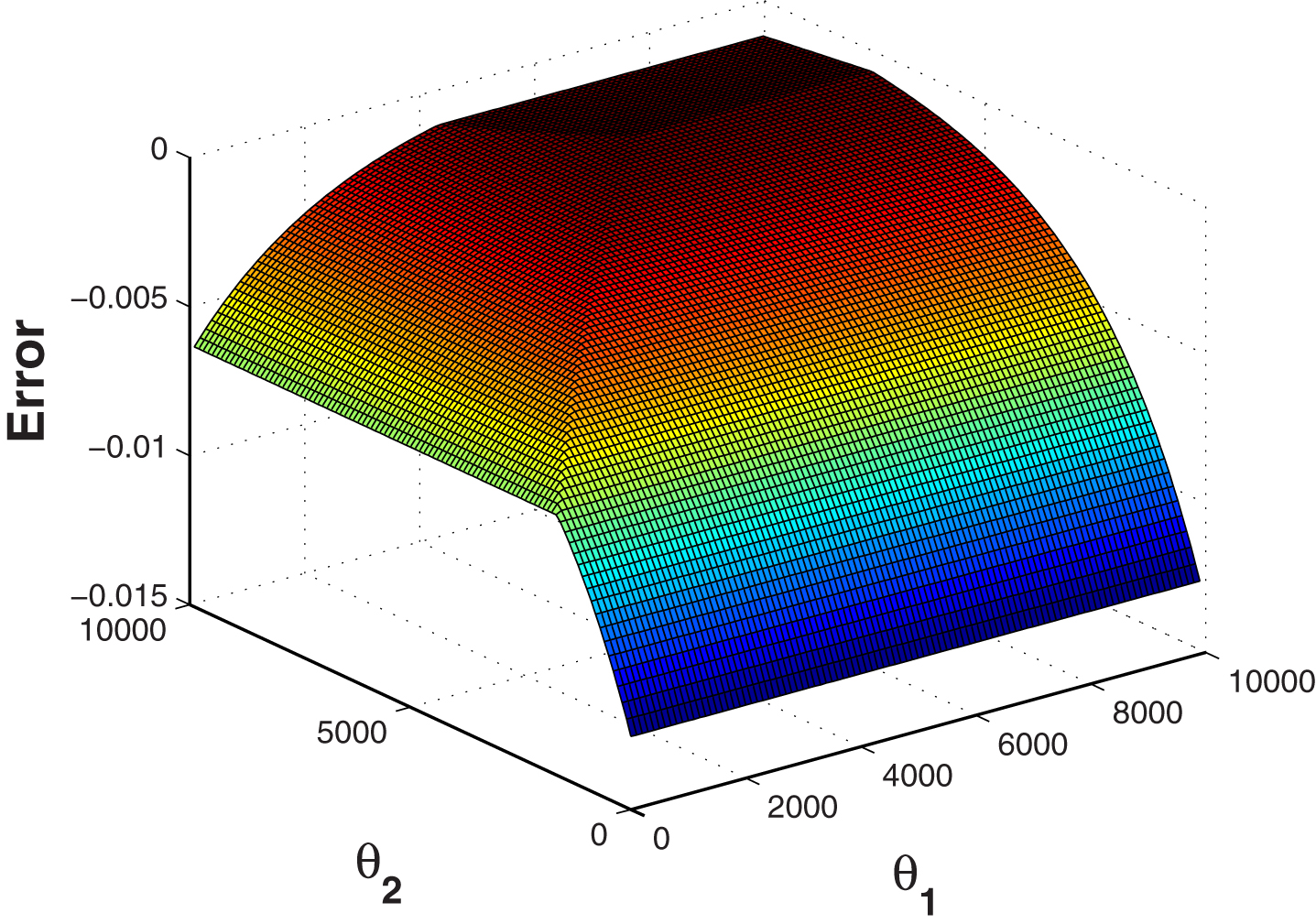
Let ɛ = 10^-10, N = 64, then we use the above difference scheme (7), (14) and (15) to solve the Example 2.1. Obviously, the binary function (16) is not a explicit formula. When θ₁, θ₂ ∈ [0, 10000], the error function $E_{ɛ}^{N} (θ_{1}, θ_{2})$ is plotted in Fig. 1. In addition, we also give the graphs of error function $E_{ɛ}^{N} (θ_{1}, 6000)$ and $E_{ɛ}^{N} (θ_{1}, 7000)$ , respectively, see Fig. 2. It is shown from Figs. 1–2 that the error function $E_{ɛ}^{N} (θ_{1}, θ_{2})$ has some local minimum value. As far as we know, the traditional optimization methods to solve problem (17) must choose a suitable initial value. However, since the range of variables θ₁ and θ₂ is too large, it is difficult to use some traditional optimization methods to find the global optimization solution. Thus, in this paper, we may choose the following basic PSO algorithm to solve the above optimization problem (17).

Fig.1

The error function -E_ɛ (θ₁, θ₂).

Fig.2

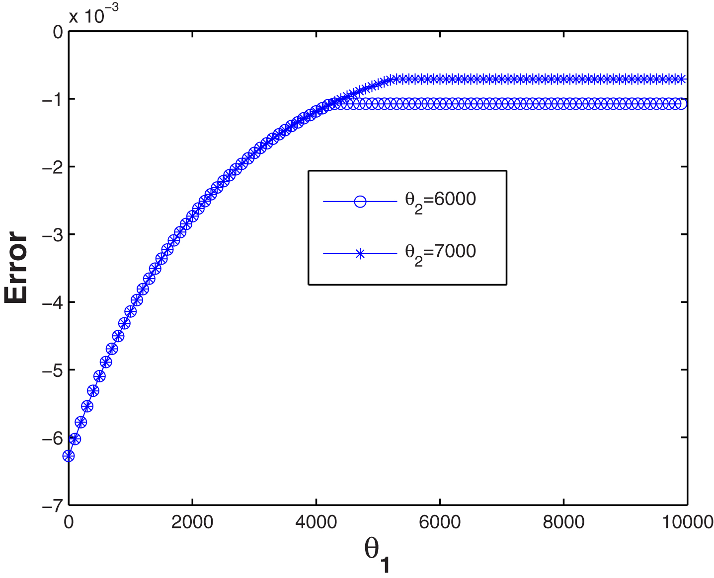
The error functions -E_ɛ (θ₁, 6000) and -E_ɛ (θ₁, 7000).

3 Particle swarm optimization(PSO)

PSO algorithm is simple yet powerful evolutionary algorithm for complicated global optimization introduced by Kennedy and Eberhart [13]. It is first developed as a new intelligence algorithm with the principle of individual improving, individual competition and population cooperation which is built upon the imitation of animal social behavior such as a bird flock [26]. It combines the local search methods so as to enhance the advantages and conquer the disadvantages of the basic algorithms and eventually obtains the global optimal solution.

A standard PSO algorithm maintains a swarm of particle and each individual is composed of three d-dimensional vectors, where d is the dimensionality of the search space [27]. The important operations of PSO algorithm are two iterative formulas on velocity and position updating in every individual. Particularly, let the velocity and the position on the ith individual in the objective space be denoted as V_i = [v_i,1, v_i,2, ⋯ , v_i,d] ^T and X_i = [x_i,1, x_i,2, ⋯ , x_i,d] ^T severally. Each historical optimal position of individual p_best is presented as P_i = [p_i,1, p_i,2, ⋯ , p_i,d] ^T, and the global optimal position g_best is formulated by using P_g = [p_g,1, p_g,2, ⋯ , p_g,d] ^T in the whole population. A mathematical model of the PSO algorithm for updating the particles’s position in each movement can be written as $\begin{matrix} v_{i, j} (k + 1) & = & ω v_{i, j} (k) + c_{1} r_{1} (p_{i, j} - x_{i, j} (k)) \\ + c_{2} r_{2} (p_{g, j} - x_{i, j} (k)), \end{matrix}$ (18) $\begin{matrix} x_{i, j} (k + 1) & = & x_{i, j} (k) + v_{i, j} (k + 1), \\ j = 1, 2, \dots, d . \end{matrix}$ (19) where c₁ and c₂ are two positive real numbers termed accelerating factors, ω is termed inertia weight factor, r₁ and r₂ are two positive random numbers for obeying standard normal distribution.

The main steps of the PSO are described as follows:

Step 1: Randomly initialize the parameters of population: population size, positions, acceleration factors, velocities, weight factor, maximum iteration number and so on.

Step 2: Compute the fitness of each individual, and select p_best in each individual and its corresponding fitness value as the local optimal solution and the local optimal value, and select g_best in the population and its corresponding fitness value as the global optimal solution and the global optimal value.

Step 3: According to Equations (18) and (19), update the corresponding velocity and position of each individual.

Step 4: Compute the fitness values of all individuals.

Step 5: Make a comparison between present fitness value and local optimal value p_best for each individual, if the present fitness is better than p_best, then replace the p_best with the present fitness.

Step 6: According to the best fitness value, we can choose the best individual of the present swarm. If the present fitness is better than g_best, then replace the g_best with the present fitness.

Step 7: If a termination criterion is satisfied, and output g_best and its fitness value; otherwise, return to Step 3.

4 Experimental studies

4.1 Problem prescription and error evaluation method

In this section, in order to validate the necessity and good performance the proposed method, the following test example is adapted. $\begin{matrix} - ɛ u^{″} (x) + u (x) \\ = - {cos}^{2} (π x) - 2 ɛ π^{2} cos (2 π x), x \in (0, 1) \end{matrix}$ with the Robin boundary conditions $\begin{matrix} u (0) - 2 \sqrt{ɛ} u^{'} (0) = 1, u (1) + 3 \sqrt{ɛ} u^{'} (1) = 0 . \end{matrix}$

Here, we use Equations (7), (14) and (15) to solve this problem. For two given parameters θ₁ and θ₂, let $U_{ɛ}^{N}$ and $U_{ɛ}^{2 N}$ be the numerical results calculated on N and 2N mesh intervals, respectively, then, we can use the following double mesh principle to estimate the error $E_{ɛ}^{N} = ∥ U_{ɛ}^{N} - U_{ɛ}^{2 N} ∥_{\infty} .$ (20)

4.2 Experimental environment and parameter setting

To facilitate the experiments, we use Matlab2012a to program a m-file for implementing the algorithms on a PC with a 32-bit windows 8 operating system, a 4GB RAM, and a 3.10 GHz-core (TM) i5-based processor.

In order to illustrate the efficient of the PSO algorithm, we also calculate the numerical results by using differential evolution (DE) algorithm, Nelder-Mead Simplex algorithm (NMS) [28] and genetic algorithm (GA) [29, 30]. The parameter settings of each stochastic algorithm are as follows:

for PSO and DE algorithm, the maximum number of generation is set to 50, the population size is also set to 50;

for PSO algorithm, two accelerating factors are set to 0.5 and 0.5, respectively. Inertia weight factor is set to 0.45;

for DE algorithm, crossover factor is 0.5,cross-over probability is 0.1;

the range of parameters θ_i (i = 1, 2) is [-10^-10, 10¹⁰].

4.3 Experimental results and analyses

4.3.1 Comparison of calculation accuracy by PSO algorithm and NMS

It is well know that many traditional optimization algorithms need the gradient information of the objective function. It is difficult to use these methods to solve above problem (16). As far as we know, the Nelder-Mead simplex (NMS) algorithm proposed by Nelder and Mead [28] is a commonly applied numerical method used to find the minimum or maximum of an objective function in a multidimensional space. It is applied to nonlinear optimization problems for which derivatives may not be known. Thus, in the experiment, we fist use NMS algorithm to solve above problem (16). First, we set the grid initial values equal to (i, i) , i = 1, 2, 3, 4, then, for different values of ɛ and N, Table 1 lists the numerical results and the corresponding grid parameters θ₁ and θ₂. It is shown that NMS method gives some local optimal solutions by choosing different initial values. Specifically, when the grid initial values equal to (1, 1), (2, 2) and (3, 3), respectively, the problem (16) has almost the same local optimal solution. Meanwhile, when we choose grid initial value (4, 4), the numerical results can reach the global optimal solution. Compared with NMS, PSO algorithm can obtain the global optimal solution without choosing grid initial value, see Tables 2–5 below (in all the tables, M denotes method).

Table 1
Numerical results calculated by using NMS method with different initial values

Initial N = 32 N = 64 N = 32 N = 64

value ɛ = 10^-8 ɛ = 10^-8 ɛ = 10^-10 ɛ = 10^-10

(1,1) $E_{ɛ}^{N}$ 3.1818e-03 6.3341e-03 3.1983e-04 2.1319e-04

θ ₁ 9.8125e-01 1.0757 1.0120 1.0688

θ ₂ 1.0531 8.7382e-01 1.0308 1.0063

(2,2) $E_{ɛ}^{N}$ 3.1810e-03 6.3334e-03 3.1983e-04 6.3935e-04

θ ₁ 2.0875 2.1296 2.1203 2.1031

θ ₂ 1.9250 2.0968 1.9382 2.0062

(3,3) $E_{ɛ}^{N}$ 3.1810e-03 4.0848e-04 3.1982e-04 6.3934e-04

θ ₁ 2.9906 7.2491e+03 3.1500 3.0000

θ ₂ 3.1828 4.8897e+03 3.0012 3.0000

(4,4) $E_{ɛ}^{N}$ 5.3787e-04 4.0848e-04 3.1980e-04 1.8213e-04

θ ₁ 5.9111e+03 7.2492e+03 4.8650 5.1260+04

θ ₂ 2.9352e+03 4.9183e+03 3.2656 8.0385e+03

Initial		N = 32	N = 64	N = 32	N = 64
(1,1)	$E_{ɛ}^{N}$	3.1818e-03	6.3341e-03	3.1983e-04	2.1319e-04
	θ ₁	9.8125e-01	1.0757	1.0120	1.0688
	θ ₂	1.0531	8.7382e-01	1.0308	1.0063
(2,2)	$E_{ɛ}^{N}$	3.1810e-03	6.3334e-03	3.1983e-04	6.3935e-04
	θ ₁	2.0875	2.1296	2.1203	2.1031
	θ ₂	1.9250	2.0968	1.9382	2.0062
(3,3)	$E_{ɛ}^{N}$	3.1810e-03	4.0848e-04	3.1982e-04	6.3934e-04
	θ ₁	2.9906	7.2491e+03	3.1500	3.0000
	θ ₂	3.1828	4.8897e+03	3.0012	3.0000
(4,4)	$E_{ɛ}^{N}$	5.3787e-04	4.0848e-04	3.1980e-04	1.8213e-04
	θ ₁	5.9111e+03	7.2492e+03	4.8650	5.1260+04
	θ ₂	2.9352e+03	4.9183e+03	3.2656	8.0385e+03

Table 2

Numerical results calculated by using different algorithms with ɛ = 10^-8, N = 32

M		Maximum error	Minimum error	Mean value	Variance
PSO	$E_{ɛ}^{N}$	5.8210e-04	5.3790e-04	5.4094e-04	6.2412e-11
	θ ₁	6.0404e+03	5.9112e+03
	θ ₂	2.6824e+03	5.0490e+03
DE	$E_{ɛ}^{N}$	3.7414e-03	2.5680e-03	2.8027e-03	2.4474e-07
	θ ₁	1.0000e+03	1.0000e+03
	θ ₂	1.0000e+08	1.0000e+03
GA	$E_{ɛ}^{N}$	3.1816e-03	3.1177e-03	3.1621e-03	4.1432e-10
	θ ₁	3.0970e-01	1.5527e-02
	θ ₂	4.4630e-01	8.1435e-01

Table 3

Numerical results calculated by using different algorithms with ɛ = 10^-8, N = 64

M		Maximum error	Minimum error	Mean value	Variance
PSO	$E_{ɛ}^{N}$	4.5077e-04	4.0885e-04	4.1557e-04	1.8056e-10
	θ ₁	7.5251e-03	7.2472e+03
	θ ₂	4.6596e-03	6.9101e+03
DE	$E_{ɛ}^{N}$	5.6721e-03	4.8463e-03	4.9053e-03	4.8719e-08
	θ ₁	1.0000e+03	1.0000e+03
	θ ₂	1.0000e+08	1.0000e+03
GA	$E_{ɛ}^{N}$	6.3353e-03	4.3765e-03	6.2337e-03	1.3739e-07
	θ ₁	9.4523e-01	6.1935e-03
	θ ₂	9.8852e-01	7.4463e-01

Table 4

Numerical results calculated by using different algorithms with ɛ = 10^-10, N = 32

M		Maximum error	Minimum error	Mean value	Variance
PSO	$E_{ɛ}^{N}$	1.1631e-04	1.1546e-04	1.1603e-04	4.7336e-14
	θ ₁	3.6656e+04	3.6878e+04
	θ ₂	2.2213e+04	2.3002e+04
DE	$E_{ɛ}^{N}$	3.1288e-02	1.1592e-04	1.4258e-03	3.8743e-05
	θ ₁	1.0000e+03	3.6757e+04
	θ ₂	1.0000e+08	1.0000e+03
GA	$E_{ɛ}^{N}$	3.1983e-04	3.1971e-04	3.1975e-04	8.2316e-16
	θ ₁	1.7969	19.6463
	θ ₂	0.7573	5.3152

Table 5

Numerical results calculated by using different algorithms with ɛ = 10^-10, N = 64

M		Maximum error	Minimum error	Mean value	Variance
PSO	$E_{ɛ}^{N}$	2.1318e-04	1.2334e-04	2.0719e-04	5.1341e-10
	θ ₁	1.3153	4.6252e+04
	θ ₂	4.0880	3.5395e+04
DE	$E_{ɛ}^{N}$	6.8735e-02	1.2304e-04	1.2360e-02	5.0793e-05
	θ ₁	1.0000e+08	4.6312e+04
	θ ₂	9.0309e+07	4.1709e+03
GA	$E_{ɛ}^{N}$	2.1319e-04	2.1317e-04	2.1319e-04	1.5651e-17
	θ ₁	2.4421e-01	2.2939e-01
	θ ₂	3.2702e-01	5.8641

Therefore, we can see that: the traditional mathematical optimization methods such as NMS method can’t be suitable for solving the above nonlinear optimization problem (17). Because those traditional mathematical optimization methods must choose a suitable initial value, and it is easy to fall into a local optimal solution.

4.3.2 Comparison of calculation accuracy by PSO and DE, GA

Here, we make a comparison of PSO algorithm with differential evolution (DE) algorithm and GA. In order to validate the effectiveness of experimental data, we perform thirty experiments by using PSO, DE and GA. algorithms to calculate this problem, respectively.

When ɛ = 10^-8 and N = 32, 64, Tables 2–3 list the max, min, average and variance of computed errors $E_{ɛ}^{N}$ by using PSO, DE and GA algorithms, respectively. Obviously, it follows from Tables 2–3 that the values of $E_{ɛ}^{N}$ calculated by using PSO is much better than that by using DE and GA. In other words, we can find the global optimal solution by using the PSO algorithm to solve the above unconstrained nonlinear optimization problems (17). At the same time, when ɛ = 10^-10 and N = 32, 64, Tables 4–5 also give the similar numerical results by using PSO, DE and GA algorithm, respectively. It can be seen from these tables that the values of $E_{ɛ}^{N}$ obtained by using PSO algorithm is also the almost smallest among the three methods. These numerical results proved that PSO algorithm has higher precision and stronger robustness compared with the DE and GA algorithms.

Figure 3 represents the absolute error curve obtained by the PSO algorithms and NMS method for N = 64, ɛ = 10^-8. Moreover, the Figs. 4–5 give the absolute error curve on the two boundary intervals. Figures 3–5 show curve graphs of the absolute error obtained by the PSO algorithm and NMS method. As can be seen from Figs. 3–5, we use the PSO to optimize the grid the transition parameters, then obtain the numerical results which are significantly higher than the those of NMS method in terms of accuracy, especially in improving the accuracy of the boundary layer with more obvious effects.

Fig.3

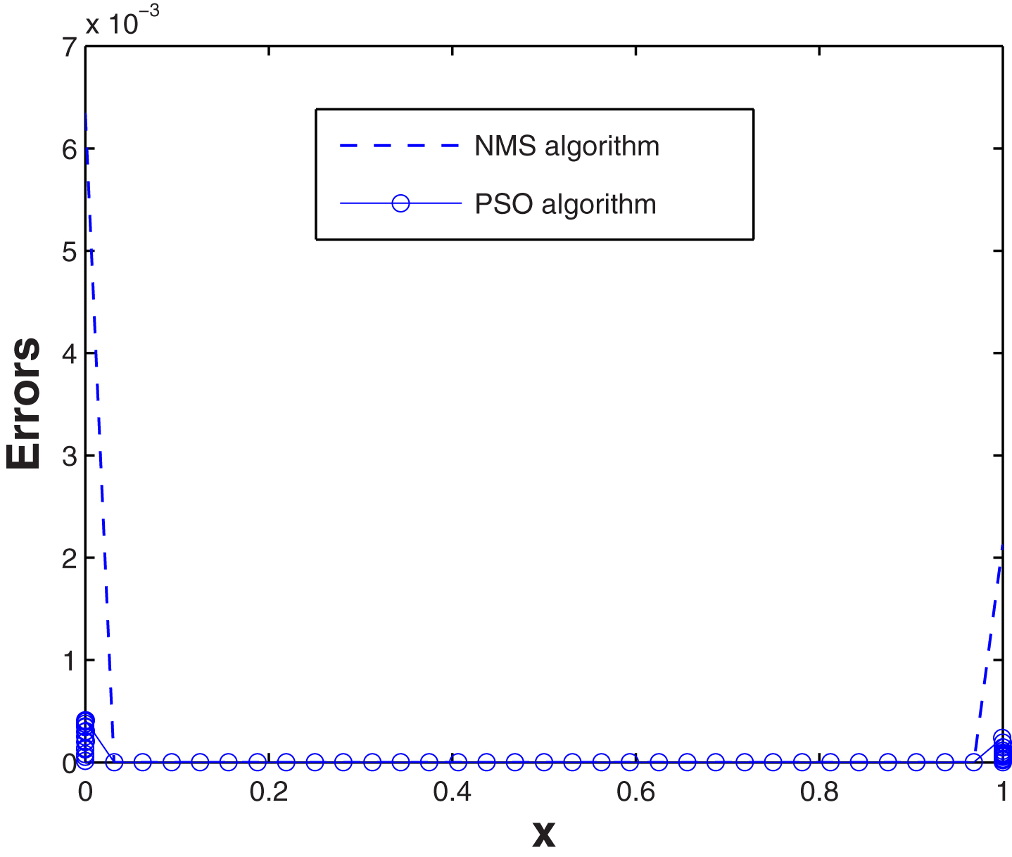
The errors comparison of PSO algorithm and NMS algorithm with ɛ = 10^-8, N = 64.

Fig.4

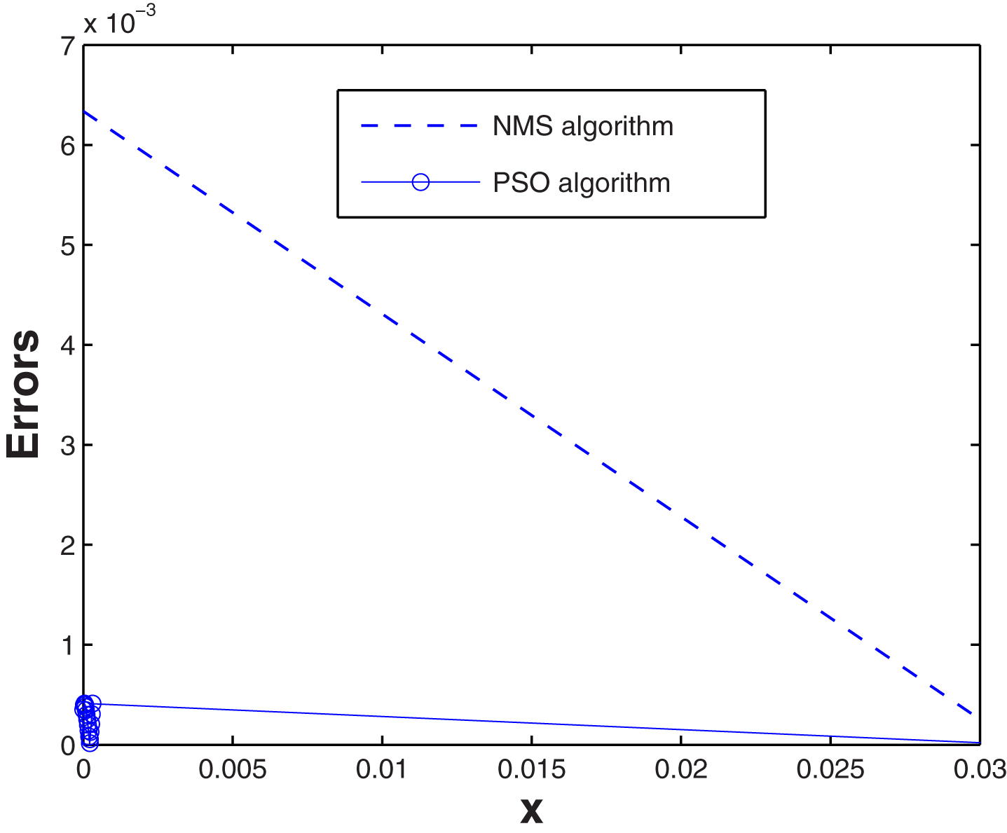
Blow-up of layer in Fig. 3 on [0, 0.03].

Fig.5

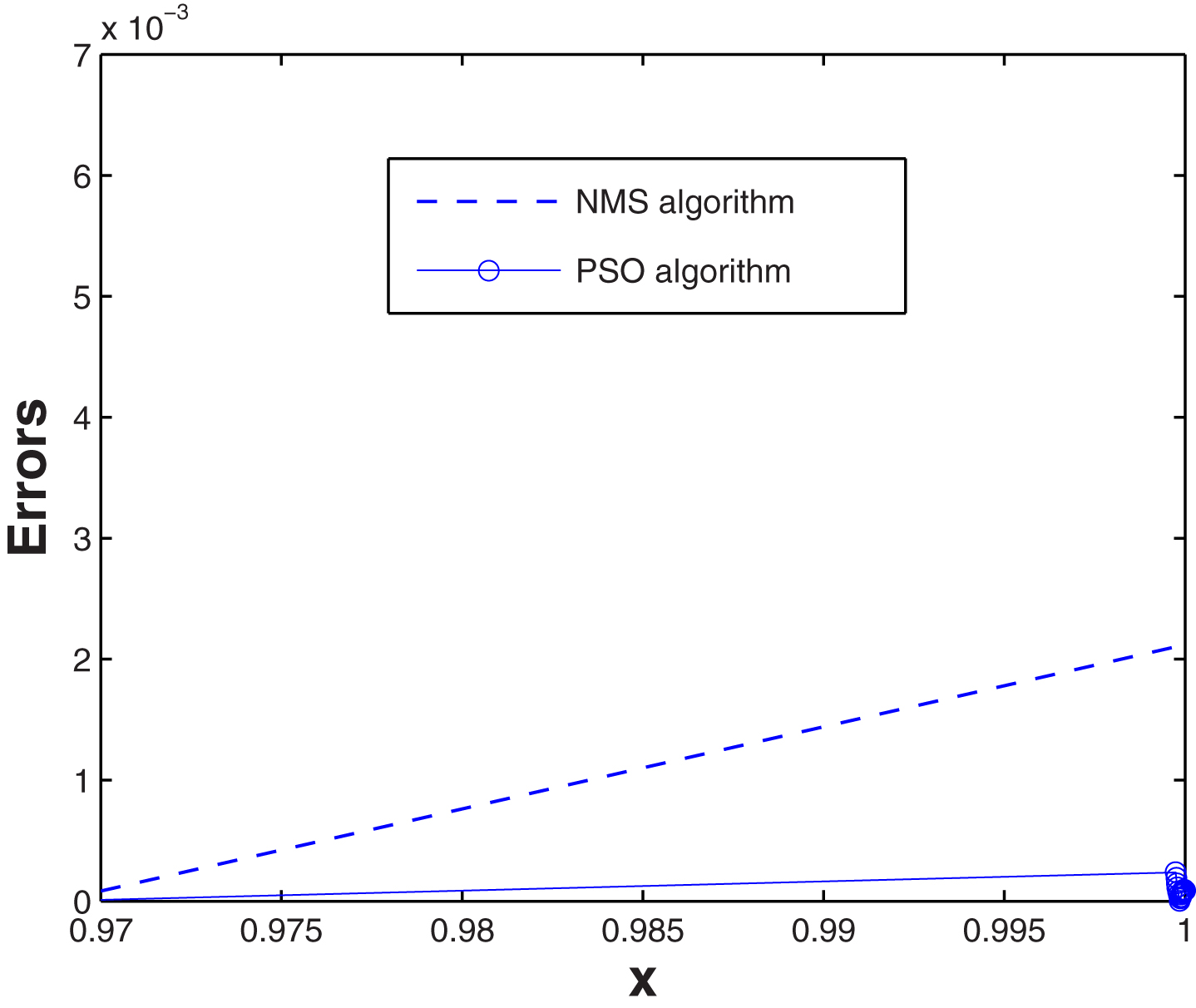
Blow-up of layer in Fig. 3 on [0.97, 1].

It is also shown from Figs. 6–7 that PSO is faster than DE and GA in terms of convergence speed.

Fig.6

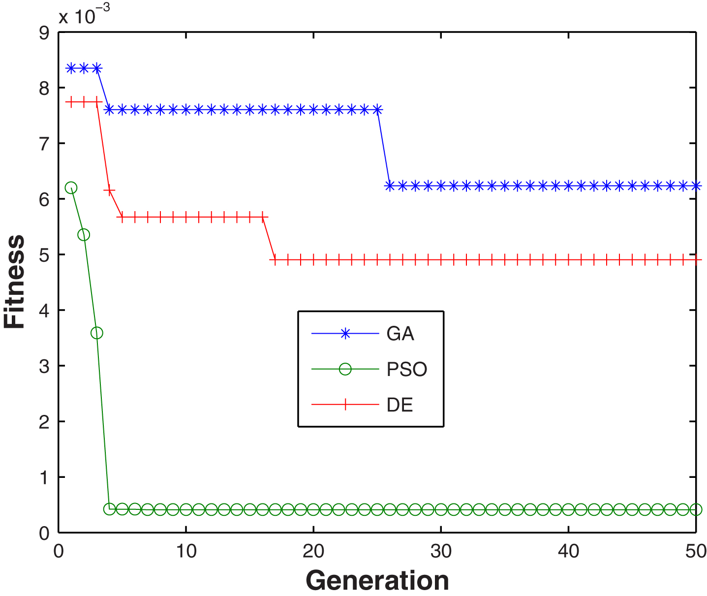
Fitness of PSO, DE and GA algorithms for generation with ɛ = 10^-8, and N = 64.

Fig.7

Fitness of PSO, DE and GA algorithms for generation with ɛ = 10^-10, and N = 64.

4.3.3 Comparison of calculation results by our method and traditional method

For the Robin boundary conditions, we compare the accuracy of our presented difference scheme (14)–(15) with that of the traditional difference scheme. At first, the construction of the traditional difference scheme is given as follow:

To approximate the first of Robin boundary conditions (3), the following center difference scheme is used $α_{1} U_{0} - β_{1} \sqrt{ɛ} \frac{U_{1} - U_{- 1}}{2 h_{1}} = γ_{1},$ (21) where U_-1 is a ghost point, outside of the region.

In addition, by applying the difference scheme (7) at the point x = x₀, we get $- ɛ \frac{U_{1} - 2 U_{0} + U_{- 1}}{h_{1}^{2}} + b_{0} U_{0} = f_{0} .$ (22)

To eliminate the U_-1 term from Equations (21)–(22), yield $\begin{matrix} (2 ɛ + b_{0} h_{1}^{2} + 2 \frac{α_{1}}{β_{1}} \sqrt{ɛ} h_{1}) U_{0} - 2 ɛ U_{1} \\ = f_{0} h_{1}^{2} + \frac{2 γ_{1}}{β_{1}} \sqrt{ɛ} h_{1} . \end{matrix}$ (23)

Similarly, for the point x = x_n, we have $\begin{matrix} - 2 ɛ U_{N - 1} + (2 ɛ + b_{N} h_{N}^{2} + 2 \frac{α_{2}}{β_{2}} \sqrt{ɛ} h_{N}) U_{N} \\ = f_{N} h_{N}^{2} + \frac{2 γ_{2}}{β_{2}} \sqrt{ɛ} h_{N} . \end{matrix}$ (24)

Here, the accuracy of difference scheme (23)–(24) is only second-order.

Next, to illustrate the advantage of our presented difference scheme (14)–(15), we use the traditional difference scheme (23)–(24) to discrete the Robin boundary conditions, and also utilize PSO algorithm to solve the objective function (17). To compare our new difference scheme i.e., our method (OM) (14)–(15) with the traditional method (TM) (23)–(24), Tables 6–9 summarize the numerical results of 30 independent runs. It is clear that our presented new difference scheme is better than the traditional difference scheme in terms of performance, which just confirms the theoretical result.

Table 6

Numerical results calculated by using different difference scheme with ɛ = 10^-2, N = 32

M		Maximum error	Minimum error	Mean value	Variance
TM	$E_{ɛ}^{N}$	1.8991e-03	1.8673e-03	1.8810e-03	1.3512e-10
	θ ₁	4.0538	3.9899
	θ ₂	6.6980	6.9150
OM	$E_{ɛ}^{N}$	4.7414e-04	4.6737e-04	4.6908e-04	4.4669e-12
	θ ₁	5.6828	5.6243
	θ ₂	7.3898	7.9278

Table 7

Numerical results calculated by using different difference scheme with ɛ = 10^-2, N = 64

M		Maximum error	Minimum error	Mean value	Variance
TM	$E_{ɛ}^{N}$	4.8483e-04	4.7032e-04	4.7562e-04	1.7470e-11
	θ ₁	3.3509	3.3352
	θ ₂	5.4900	5.7774
OM	$E_{ɛ}^{N}$	1.1996e-04	1.1858e-04	1.1907e-04	1.9238e-13
	θ ₁	4.5748	4.5410
	θ ₂	6.2679	6.7097

Table 8

Numerical results calculated by using different difference scheme with ɛ = 10^-4, N = 32

M		Maximum error	Minimum error	Mean value	Variance
TM	$E_{ɛ}^{N}$	6.8082e-03	6.6177e-03	6.6458e-03	3.3116e-09
	θ ₁	9.2053e+01	9.0302+01
	θ ₂	6.1827e+01	9.4059+01
OM	$E_{ɛ}^{N}$	2.7831e-03	2.5781e-03	2.6205e-03	6.4589e-09
	θ ₁	1.2004e+02	1.1572e+02
	θ ₂	8.6874+01	1.3570e+02

Table 9

Numerical results calculated by using different algorithms with ɛ = 10^-4, N = 64

M		Maximum error	Minimum error	Mean value	Variance
TM	$E_{ɛ}^{N}$	2.4503e-03	2.4243e-03	2.4337e-03	5.9503e-11
	θ ₁	9.2421e+01	9.1858+01
	θ ₂	7.1511e+01	9.6488+01
OM	$E_{ɛ}^{N}$	1.0437e-03	1.0041e-03	1.0188e-03	2.8995e-10
	θ ₁	1.1386e+02	1.1166e+02
	θ ₂	8.9961+01	1.1444e+02

5 Concluding remarks

In most of the cases, the Shishkin mesh method is frequently used to solve the singularly perturbed problem. However, for the Shishkin mesh transition points, almost all of authors are arbitrary selection parameters. Thus, the mainly advent of this paper has provided a new approach to obtain the Shishkin mesh transition points. This work can be viewed as a preliminary step-up in finding a challenging numerical method to obtain the Shishkin mesh transition points.Specially, we first transform the Shishkin mesh transition parameter selection problem into a nonlinea unconstrained optimization problem which is solved by using the basic particle swarm optimization (PSO) algorithm. Then, for the Robin boundary conditions, a high precision discrete scheme is developed. It is noted that the method used in this paper can be extend to other type of singularly perturbed problems.

Footnotes

Acknowledgements

This work is supported by National Science Foundation of China (11461011, 61662090, 11561009), and Natural Science Foundation of Guangxi Education Department in China (ZD2014080), and Guangxi Natural Science Foundation (2016GXNSFAA380240). the High-level Innovative Talents Cultivation Program of Guizhou Province (No. [2017]3), the Natural Science Foundation of Guizhou Provincial Education Department (No. KY[2016]018), the Science and Technology Research Foundation of Hunan Province (13C333), the open fund of Key Laboratory of Guangxi High Schools for Complex System & Computational Intelligence (No. 15CI03D).

References

Chang

K.W.

and Howes

F.A.

, Nonlinear Singularly Perturbation Phenomena: Theory and Application, Springer, New York, 1984.

Linß

, Maximum-norm error analysis of a nonmonotone fem for a singularly perturbed reactiondiffusion problem, BIT Numerical Mathematics 47 (2007), 379–391.

Cai

, Cai

D.L.

, Wu

R.Q.

, et al., High accuracy non-equidistant method for singularly perturbation reaction-diffusion problem, Appl Math Mech 30 (2009), 175–182.

Kumar

, High order compact finite difference scheme for singularly perturbed reaction diffusion problems on a new mesh of Shishkin type, J Optim Theory Appl 143 (2009), 123–147.

Linß

, Radojev

and Zarin

, Approximation of singularly perturbed reaction-diffusion problems by quadratic C¹ splines, Numer Algor 61 (2012), 35–55.

Vulanović

and Teofanov

, A modificaion of the Shishkin discretization mesh for one-dimensional reaction-diffusion problems, Appl Math Comput 220 (2013), 104–116.

Natesan

and Bawa

R.K.

, Second-order numerical scheme for singularly perturbed reaction-diffusion Robin problems, J Numer Anal Ind Appl Math 2 (2007), 177–192.

Dai

W.Z.

and Tzhou

D.Y.

, A fourth-order compact finite difference scheme for solving an N-carrier system with Neumann boundary conditions, Numer Methods Partial Differential Eq 26 (2010), 274–289.

Dai

W.Z.

, A new fourth-order difference scheme for solving an N-carrier system with Neumann boundary conditions, Numer Methods Partial Differential Eq 27 (2011), 436–446.

10.

Liu

L.B.

and Liu

H.W.

, A new fourth-order difference scheme for solving an N-carrier system with Neumann boundary conditions, Int J Comput Math 88 (2011), 3553–3564.

11.

Liu

L.B.

, Liu

H.W.

and Chen

, Polynomial spline approach for solving second-order boundary-value problems with Neumann conditions, Appl Math Comput 217 (2011), 6872–6882.

12.

Liu

L.B.

and Liu

H.W.

, Compact difference schemes for solving telegraphic equations with Neumann boundary conditons, Appl Math Comput 219 (2013), 10112–10121.

13.

Kennedy

and Eberhart

R.C.

, Particle swarm optimization, in: Proceeding of the IEEE international Conference on Neural Networks (Perth, Australia), IEEE Service Ceter, Piscataway, NJ, 1995, pp. 1942–1948.

14.

Menhas

M.I.

, Wang

, Fei

, et al., Comparative performence analysis of various binary coded PSO algorithms in multivariable PID controller design, Expert, Syst Appl 39 (2012), 4390–4401.

15.

Ouyang

, Li

, Truong

T.K.

, Sallam

and Sha

E.H.M.

, Hybrid particle swarm optimization for parameter estimation of Muskingum model, Neural Computing and Applications 25(7-8) (2014), 1785–1799.

16.

Al-geelani

N.A.

, Piah

M.A.M.

, Adzis

, et al., Hybird regroupling PSO based wavelet neural networks for characterization of acoustic signals due to surface discharges on H.V. glass insulators, Appl Soft Comput 13 (2013), 4622–4632.

17.

Chander

, Chatterjee

and Siarry

, A new social and momentum component adaptive PSO algorithm for image segmentation, Expert Syst Appl 38 (2011), 4998–5004.

18.

Subasi

, Classfication of EMG signals using PSO optimized SVM for diagnosis of neuromuscular disorders, Comput Biol Med 43 (2013), 576–586.

19.

Saidi

, Khelil

, Hassouni

, et al., Energy spectra of the Schrödinger equation and the differential quadrature method: Improvement of the solution using particle swarm optimization, Appl Math Comput 182 (2006), 559–566.

20.

Lee

Z.Y.

, Method of bilaterally bounded to solution Blasius equation using particle swarm optimization, Appl Math Comput 179 (2006), 779–786.

21.

Pérez

, Amaya

and Correa

, Numerical solution of certain exponential and non-linear Diophantine system of equations by using a discrete particle swarm optimization algorithm, Appl Math Comput 225 (2013), 737–746.

22.

Babaei

, A general approach to approximate solutions of nonlinear differential equations using particle swarm optimization, Appl Soft Comput 13 (2013), 3354–3365.

23.

Ouyang

, Tang

, Zhou

, Xu

, Pan

and Li

K.Q.

, Parallel hybrid PSO with CUDA for lD heat conduction equation, Computer & Fluids 110 (2015), 198C210.

24.

Karr

C.L.

and Wilson

, A self-tuning evolutionary algorithm applied on an inverse partial differential equation, Appl Intell 19 (2003), 147–155.

25.

Reich

, Simulation of imprecise ordinary differential equations using evolutionary algorithms, Proceedings of the 2000 ACM Symposium on Applied Computing, 1, 2000, pp. 428–432.

26.

and Wang

, A hybrid particle swarm optimization with a feasibility-based rule for constrained optimization, Appl Math Comput 186 (2007), 1407–1422.

27.

Ouyang

, Tang

, Li

, Sallam

and Sha

, Estimating parameters of Muskingum model using an adaptive hybrid PSO algorithm, International Journal of Pattern Recognition and Artificial Intelligence 28(01) (2014), Article ID 1459003.

28.

Nelder

J.A.

and Mead

, A simplex method for function minimization, Comput J 7 (1965), 308–313.

29.

, Li

, Hu

and Li

, A genetic algorithm for task scheduling on heterogeneous computing systems using multiple priority queues, Information Sciences 270 (2014), 255–287.

30.

, Li

, He

, Zhang

and Li

, A hybrid chemical reaction optimization scheme for task scheduling on heterogeneous computing systems, IEEE Transactions on parallel and Distributed Systems 26(12) (2015), 3208–3222.