
Abstract
In recent years, due window assignment scheduling problems deriving from just-in-time supply chain management have been studied extensively. However, precedence constraints and uncertain processing times of jobs are rarely involved simultaneously in the studies. In this paper, a single machine due window assignment scheduling problem with uncertain processing times, precedence constraints and due window size constraints is investigated, in which the processing times of jobs are presented by fuzzy numbers. The objective is to minimize the mean value of the total earliness-tardiness penalties. An optimal polynomial time algorithm is proposed for the problem when there are no precedence constraints among jobs. Note that the problem with general precedence constraints is NP-hard. An efficient 2-approximation algorithm is proposed for the general constraint problem based on linear programming relaxation. The experimental results show that the proposed methods are effective and promising.
Keywords
Introduction
Just-In-Time (JIT) philosophy is usually adopted in the supply chain management by modern enterprises to reduce their inventor costs, helping them to provide higher quality of services and improve their competitive advantages in the global market. It is extensively accepted that the scheduling strategy plays a crucial role in the realization of JIT in a manufacturing environment [1]. One important goal of JIT scheduling model is to discourage early and tardy jobs so as to minimize the earliness-tardiness penalties [24].
In practice, when a customer signs a contract with a supplier, a due date or generally a due window is often specified according to the negotiation between them. It is usually a compromise between the customer’s expectation and the supplier’s estimation that is mainly based on its production schedule [24]. The left end, the right end and the length of the window are called the starting time, the finishing time and the due window size, respectively. If a job is finished in the due window, it is considered to be on time and will not result in any penalty. If a job is completed before the starting time of the due window, it incurs an earliness penalty which usually includes inventory carrying cost, holding cost, and insurance cost. Alternatively, if a job is finished after the finishing time of the due window, it brings about a tardiness penalty which may include loss of customer goodwill, late charges, and loss of sales. Hence, in order to avoid such penalties, it is very important for the enterprises to obtain an optimal production schedule and determine the reasonable due windows for all jobs at the negotiation stage. Such problems are well-known as the due window assignment scheduling problems, which are studied extensively by many scholars [3, 27]. Cheng et al. [23] investigate the problem of common due window assignment and scheduling of deteriorating jobs and a maintenance activity simultaneously on a single machine. Yin et al. [27] address a single machine batch delivery scheduling problem with an assignable common due window. Liu et al. [16] study a single machine due window assignment and resource allocation scheduling problem with learning and general positional effects. Yang et al. [6] examine some multiple due windows assignment scheduling problems with controllable processing times on a single machine. Janiak et al. [3] consider a due window assignment schedule problem on parallel machines with min-max type criteria, where the time complexity is strong NP-hard. Gerstl and Mosheiov [8] study a due window assignment scheduling problem on parallel uniform machines with job-dependent earliness-tardiness costs. An improved algorithm is then given for the same problem [7]. Yeung et al. [26] investigate a two machine common due windows proportionate flow shop scheduling problem.
However, in many practical applications, the data for the processing times of jobs are usually recorded or collected under the influence of some unexpected noises. Hence, the processing times of jobs are not known exactly in advance. Additionally, the historical data are not abundant for the processing times of jobs to get the probability distributions, which makes it difficult to model the due window assignment scheduling problems by the stochastic models given in [13, 25]. Furthermore, the intuition and the judgement of a experienced worker play an important role in determining the processing time of a job in practice. For example, a job’s processing time perhaps is approximately 3 hours according to the evaluation of a experienced worker, which can be expressed by fuzzy number
Note that, due to the uncertainty inherent scheduling problems, the completion time of a job can not be exactly predicted in advance, but be estimated to lie in a time interval. Hence, there are usually no penalties when the job is completed within a time interval rather than a time point in real-life applications [2]. For example, a time interval usually should be promised by the supplier to deliver goods to the customer, not an exact timing due to the uncertainty. Also, there are more complex precedence constraints between jobs [9, 22]. Hence, it is necessary to study the due window assignment scheduling problems with uncertain processing times and general precedence constraints among jobs. In this direction, this paper investigates the due window assignment problem with fuzzy processing times, general precedence constraints and due window size constraints on a single machine. The objective is to find an optimal job sequence under precedence constraints and determine an optimal due window with due window size constraint for each job such that the crisp possibilistic mean (or expected) value of the total earliness-tardiness penalties is minimized. An optimal polynomial time algorithm is put forward for the considered problem with no precedence constraints among jobs. Note that the problem with general precedence constraint is NP-hard. An efficient 2-approximation algorithm is presented for the general constraint problem based on solving a linear programming relaxation of this kind of scheduling problems. Finally, the numerical experiment is given, whose results show that our methods are promising.
The properties and algorithms for the problem
Preliminaries
A fuzzy number
The arithmetic operations of fuzzy numbers based on the extension principle are given in [17] as follows. For
The graphical representations are given for the calculations above with fuzzy numbers in Fig. 1.
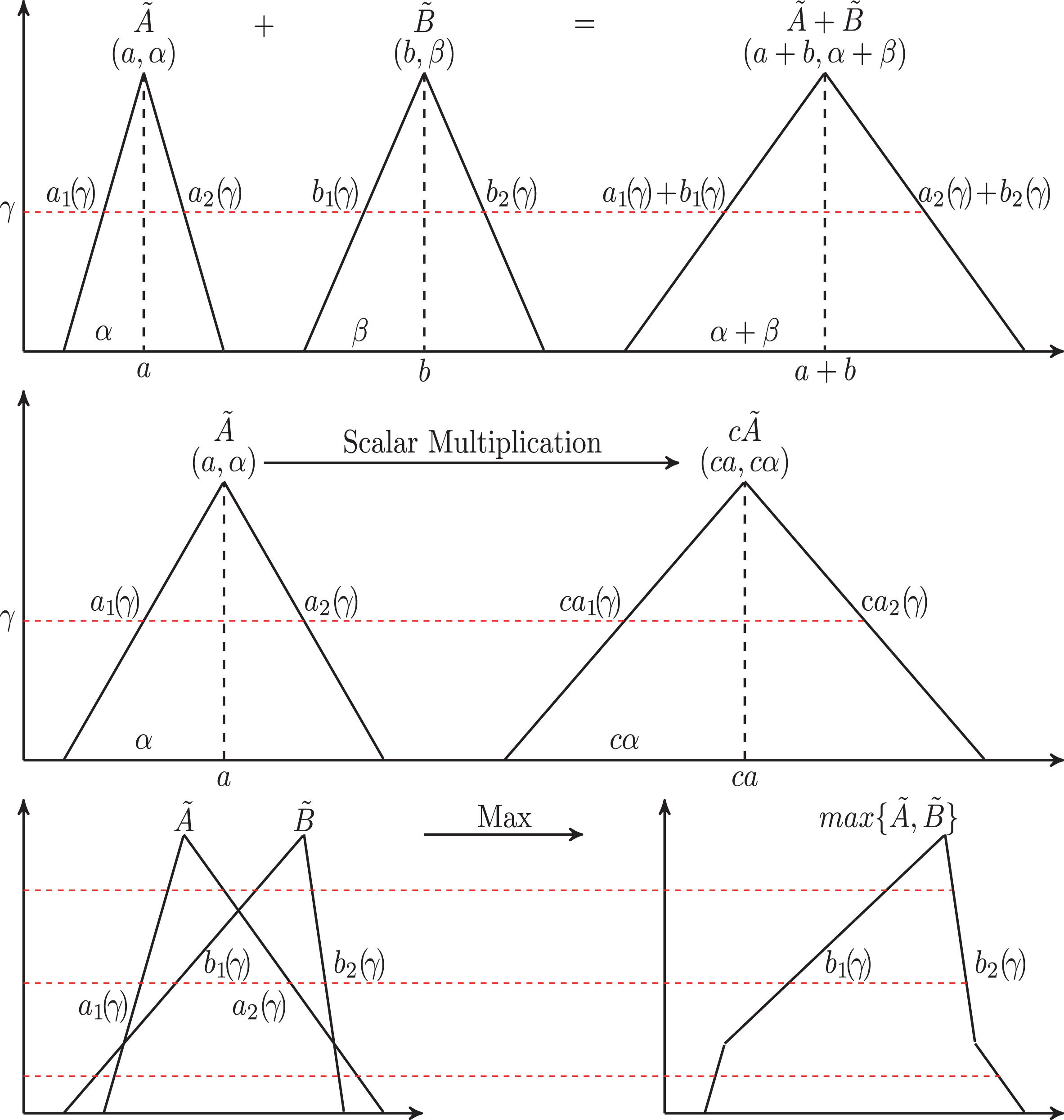
The graphical representation for calculations with
The standard deviation of
By the arithmetic operations of fuzzy numbers and Definition 1, it is easy to get that
In [5], a triangular fuzzy number
When α = β, the triangular fuzzy number is called the symmetric triangular fuzzy number denoted by (a, α).
As it is pointed out in [5], the crisp possibilistic mean value and variance for
In this paper, a single machine due window assignment scheduling problem is investigated, in which the jobs have to be processed on a single machine and the scheduler determines a due window for each job in uncertain environment. All jobs are available at time zero; the preemption of jobs and the idle machine times are not allowed; the machine can process at most one job at a time; there are precedence constraints among jobs; the uncertain processing times are modeled by the symmetrical triangular fuzzy numbers. The problem notations used in this paper are presented as follows:
<d i , d i + L i >: due window of job J i with the beginning time d i > 0 and the size L i > 0;
e i > 0: per unit earliness penalties;
t i > 0: per unit tardiness penalties.
The precedence constraints among jobs in the field of scheduling are usually specified in the form of a directed acyclic graph G, in which each vertex represents a job. We say that J i precedes J j or J j succeeds J i , written as J i → J j , whenever there is a directed path from vertex J i to vertex J j in G [14].
Note that, there are many factors affecting the due window size of a job, such as the customer’s demand, the uncertain processing time and the machine’s speed. The most important factor is the uncertainty of the completion time, which means that the due window size is strongly influenced by the standard deviation of the completion time. Usually, a wide due window is not acceptable, since a large due window and delayed job completion reduce the enterprise’s competitiveness and customer service level. Thus, it is necessary to give a constraint for the size of a due window. In this paper, it is assumed that, for each job, there is a linear constraint between the due window size and the standard deviation of the completion time, that is
Extending the standard scheduling notations [12, 20], this problem is denoted as
Especially, when there are no precedence constraints among jobs, the problem is denoted as
By computation, g (k) = αh (e, t, λ, k), where
According to Equation (12), the function g (k) is a cubic piecewise polynomial of k in [−1 − λ, 1]. Hence we can obtain k* that minimizes g (k) by the following algorithm:
Step 1. Find the derivative g′ (k) of the cubic piecewise polynomial g (k) in the set R − {−1 − λ, − 1, − λ, 0, 1 − λ, 1}.
Step 2. Find the roots of the derivative g′ (k) if exist.
Step 3. Compute the value of the function g (k) in the set A = {k|g′ (k) =0} ∪ {−1 − λ, − 1, − λ, 0, 1 − λ, 1}.
Step 4. Find the minimal value g (k*) of the set {g (k) |k ∈ A} and return k*.
According to Lemma 1 and Algorithm 1, we can assign the optimal due window <a+ k*α, a + (k* + λ) α > to the job with the given the completion time
According to Definition 5, <d*, d*+ L > is an optimal due window with respect to the completion time
Let
Furthermore, without loss of generality, let π = (J1, J2, ⋯, J
n
). Then the completion time of job J
i
is
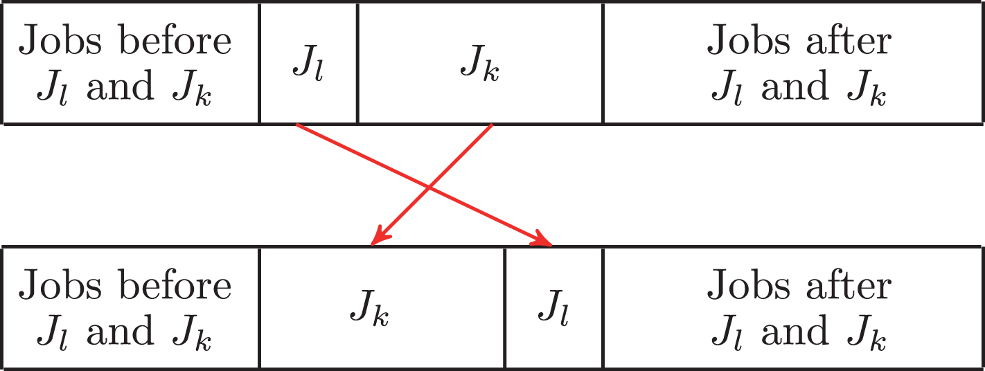
The adjacent pairwise interchange of J l and J k .
Known from Lemma 3, it is a necessary condition for an optimal schedule that
In the rest of the paper,
Step 1. Input fuzzy processing time (a i , α i ), per unit earliness penalties e i , per unit tardiness penalties t i and due window size ratio λ i for job J i (i = 1, ⋯, n).
Step 2. Compute the optimal customer service level k i by Algorithm 1 and the unitary comprehensive penalty w i under k i and λ i by w i = h (e i , t i , λ i , k i ) (i = 1, ⋯, n).
Step 3. Schedule the jobs according to the nonincreasing order of w i /α i . The schedule is denoted as π.
Step 4. Compute the completion time
Step 5. Return π,
Note that, with a general constraints among jobs, the problem
For the problem
By Definition 1, it is easy to get
According to Equation (13), for a schedule π with the customer service levels
Note that Equation (18) is not linear inequalities. However, for a feasible scheduling π = {Jπ(1), Jπ(2),⋯, Jπ(n)} of jobs set
Based on the above linear inequalities, using the standard deviations of the completion times as the variable, a linear programming relaxation of the problem 1
Based on the linear programming above, an algorithm is designed for the problem 1
Step 1. Input fuzzy processing time (a i , α i ), unit earliness penalties e i , unit tardiness penalties t i , due window size ratio λ i for job J i (i = 1, ⋯, n). Input precedence constraints G among jobs.
Step 2. Compute the optimal customer service level k i by Algorithm 1 and the unitary comprehensive penalty w i under k i and λ i by w i = h (e i , t i , λ i , k i ) (i = 1, ⋯, n).
Step 3. Construct the linear programming induced by 1
Step 4. Solve the linear programming problem of step 3 and obtain the solution
Step 5. Schedule the jobs according to the nondecreasing order of
Step 6. Compute the completion time
Step 7. Return π,
On the other hand, for an optimal schedule π* = {Jπ*(1), Jπ*(2), ⋯, Jπ*(n)} with

The precedence constraint for Example 1.
First, compute the unitary comprehensive penalty under optimal customer service level for each job, that is
Next, schedule the jobs according to the nondecreasing order of

The Gantt chart of the schedule obtained by Algorithm 3 for the fuzzy completion times in Example 1.
The due windows of all jobs are <5.1076, 5.7076>, <15.8400, 19.4400 >, <49.5474, 57.1474 >, <55.2417, 59.8417 >, <3.2364, 3.4364 >, <8.0890, 10.4890 >, <29.8068, 35.6068 >, <24.2278, 26.1278 >, #x003C;11.9386, 15.1386 >, <19.3307, 23.8307 >, <60.2251, 68.6251 >, <24.2867, 29.0867 > and <42.3958, 52.8958>, respectively.
For the scheduling problems with uncertain processing times, stochastic methods are use to model the problems, where the processing times are usually assumed as random variables with normal distributions [25]. According to the results of [25], a due date d can be assigned to a job such that the expected value of the earliness-tardiness penalties E (e max {d − C, 0} + t max {C − d, 0}) is minimized, whose completion time is a random variable C with a normal distribution N (μ, σ2). Similarly, a due window <d, d+ L > can be obtained such that the expected value of the earliness-tardiness penalties E (e max {d − C, 0} + t max {C − d − L, 0}) is minimized, and it is detailedly given out how to determine the due window <d, d+ L > in Appendix, which is an extension of the results in [25]. Without special statement, the above method extending from [25] and the method of our paper are briefly written as the stochastic method and the fuzzy method in the following.
Next, the stochastic method and the fuzzy method will be tested on the same data come from Example 1 [25] to examine their effectivity by comparing the total penalties, which can be denoted by the flow diagram in Fig. 5.

The flow diagram for examining the effectivity of the due window assignment method.

The earliness-tardiness penalty of each job in samples 1–6.
In Example 1 [25], the processing time of the job is a random variable with the normal distribution N (10, 32); the per unit earliness penalties and tardiness penalties are
Then, model the uncertain processing time of the job by the uncertain variables based on the sampled data and determine the job’s due windows with the size L = 3 by the use of two methods. For the stochastic method, the uncertain processing time of the job is modeled by a random variable with the normal distribution N (10, 32) for each sample, and the optimal due window is <11.3280, 14.3280>, where the solving process is given in Appendix; for the fuzzy method of our paper, the uncertain processing time of this job for each sample is modeled by a symmetrical triangle number (10, 8.5), since the processing time of the job is almost in the interval [1, 19] according to the 3σ principe; and the optimal due window is <12.1068, 15.1068> according to the fuzzy method of this paper.
The total penalties of sample 1–sample 6
Then, compute the earliness-tardiness penalties of all jobs in each sample based on the collected data, which are are shown in Fig. 6. Also, compute the total penalties of all jobs in each sample for these two methods, and compute the decreasing rates of the total penalties for the fuzzy method compared to the ones for the stochastic method, which are given in Table 1 for 6 samples; Known from the decreasing rates of all samples in Table 1, for the same data above, the total penalties induced by the due window obtained by our method are less than the ones induced by the due window obtained by stochastic method.
Further, our model can deal with the due window assignment scheduling problems with general precedence constraints among jobs under uncertain environment, whereas there are no results for this case by stochastic method as far as we know. Moreover, we use Example 1 in section 2 to test Algorithm 3. All algorithms are implemented using MATLAB language (no explicit use of parallel toolbox), tested in MATLAB 2017b, 16 GB memory and Intel core i7-7700 CPU. Then, the schedule with the objective function value 403.2450 is obtained by Algorithm 3 in 3 seconds. On the other side, the optimal schedule π* is (J5, J1, J6, J9, J2, J10, J8, J12, J7, J3, J13, J11, J4) with the objective function value 402.7872 can be obtained by the enumeration, but the time is about 1890 seconds due to examining 39916800 permutations. Moreover, the ratio of two objective function values is
In this paper, a single machine due window assignment scheduling problem with precedence constraints in fuzzy environment was studied. The optimal polynomial time algorithm for
However, Algorithm 3 is required to solve a kind of linear programming with exponentially large class of constraints. Our work may accordingly focus on designing more effective algorithm for the due window assignment scheduling with general precedence constraints and fuzzy processing times.
Appendix
In the following, it is illustrated how to obtain <d, d + L > 0 such that the expected value of the earliness-tardiness penalties E (t max {ξ − d − L, 0} + e max {d − ξ, 0}) reaches the minimal value, where e, t, L > 0 and ξ ∼ N (μ, σ2) with the probability density function
Let Y = max {ξ − d − L, 0} and Z = max {d − ξ, 0}. Then, it follows that
Hence, the probability density functions of Y and Z are
Then, it is not difficult to get
It follows that
It is easy to verify that and G (d) is a convex function on (− ∞, + ∞) with
In fact, for t ≠ e, it is not easy to get the analytical solution of the equation:
The numerical solution of can be obtained by numerical method. In this paper, Newton iteration method is used to solve the with the iteration equation for Example 1.
Footnotes
Acknowledgments
This paper was supported by National Natural Science Foundation of China (11401030), the Training Program of Outstanding Young Teacher for Guangdong’s Colleges and Universities (2014) and Teacher Research Capacity Promotion Programm of Beijing Normal University Zhuhai.