Supply chain coordination with controllable lead time under imperfect production process

Abstract

This article discusses a vendor-buyer inventory model with permissible delay in payments and controllable lead time in which the order quantity, lead time and the number of shipments delivered from vendor to the buyer in a production cycle are decision variables. Here the production process is imperfect. The lead time is crashed and the crashing cost is an exponential function of lead time. Based on the lead time demand, two models are developed, that is, lead time demand follows a normal distribution in the first model and then distribution free approach is considered in the second model to minimize the joint total expected cost per unit time. Efficient computational algorithm is designed to find the optimal solution. Numerical examples are provided to illustrate the results obtained. Sensitivity analysis is carried out to study the changes in the effect on optimal solution and some managerial phenomena are obtained through sensitivity analysis.

Keywords

Supply chain controllable lead time permissible delay in payment service level constraint

1 Introduction

A supply chain is a network of facilities that procure raw materials, transform them into intermediate goods and then final products, and finally deliver the products to customers through a distribution system that includes an inventory system [1]. Traditionally, the study of integrated vendor-buyer management has attracted considerable attention, accompanying the growth of Supply Chain Management (SCM). SCM is the oversight of materials, information and finances as they move in a process from supplier to manufacturer to wholesaler to retailer to consumer. SCM involves coordinating and integrating these flows both within and among companies. Integrated supply chain management has been gradually recognized as a core competitive strategy, since enterprises continuously seek to provide products and services to customers faster, cheaper, and better than their competitors [2]. Hill [3] developed an integrated single-vendor single-buyer production inventory model with a generalized policy. Sarmah et al. [4] gave an intended literature review to cover the entire gamut of supply chain coordination mechanism. The purpose of this article is to formulate a single vendor single buyer integrated inventory model for defective items with controllable lead time. This paper considers imperfect production processes and delay in payments. An inspection policy is used to identify the defective items. The lead time crashing cost per order is assumed to be an exponential function of lead time. The lead time demand follows a normal distribution and then we apply the distribution free approach to minimize the joint total expected cost per unit time. Our article optimizes an integrated inventory system by employing the mathematical model with variable lead time and service level constraint. Computational algorithms are framed to determine the optimal solution. Numerical examples are provided to illustrate the solution procedure. Managerial implications are discussed in detail with the help of sensitivity analysis carried.

2 Literature review

The cooperation between vendor and buyer for improving the performance of inventory control has received a great deal of attention, and the integration approaches were studied for years. Yao et al. [5], Zhang et al. [6], Huang et al. [7] gave an integrated vendor-buyer inventory models. Rau and Ouyang [8] considered an optimal batch size for integrated production inventory policy in a supply chain. Lin and Ho [9] developed an integrated inventory model with quantity discount and price sensitive demand. Chung [2] derived an integrated vendor-buyer production inventory model with backordering using cost-difference rate comparison approach. It is common yet unrealistic to assume that all the units produced are of good quality. The classical Economic Order Quantity (EOQ) model such as Jaggi et al. [10], Geetha and Udayakumar [1, 11], Baten and Khalid [12, 13], Udayakumar and Geetha [14 –16] assume that items produced are of perfect quality, which is usually not the case in real production. Huang [17] developed an integrated inventory model for supplier and retailer with defective items. In his article, he incorporates the view of the integrated supplier-retailer approach into the inventory model with imperfect items to determine the optimum ordering quantity and number of deliveries per order. Goyal et al. [18], Sana [19], Lin and Lin [20], Ouyang et al. [21] developed vendor-buyer inventory model for defective items. Hsu and Hsu [22] developed an integrated vendor-buyer cooperative inventory model in an imperfect production process with shortage backordering.

An important component of an inventory model is the lead time, which is the amount of time between the placement of an order to replenish inventory and the receipt of the goods into inventory systems. When the demand during the cycle period is not deterministic but is stochastic, lead time becomes an important issue and its control leads to many benefits. In some practical situations, lead time and ordering cost can be controlled and reduced in various ways. The lead time can be reduced by an additional crashing cost. In this direction, Goyal [23], Ouyang et al. [24, 25], Daya and Hariga [26], developed an integrated vendor-buyer cooperative model with controllable lead time. Jha and Shanker [27] gave a single vendor-buyer production inventory model with controllable lead time and service level constraint for decaying items. Lin [28] developed an integrated vendor-buyer inventory model with backorder price discount and effective investment to reduce ordering cost.

Trade credit is an important external source of working capital financing. It is a short-term credit extended by suppliers of goods and services in the normal course of business, to a buyer in order to enhance sales. Trade credit arises when a supplier of goods or services allows customers to pay for goods and services at a later date. Ho et al. [29] gave an optimal pricing, shipment and payment policy for an integrated supplier–buyer inventory model with two-part trade credit. Ouyang et al. [30] established an optimal strategy for an integrated system with variable production rate when the freight rate and trade credit are both linked to the order quantity. Researchers like Chen and Kang [31], Huang et al. [32], Su [33], Soni and Patel [34] gave integrated inventory model under trade credit policies. Uthayakumar and Priyan [35] derived two echelon inventory models with controllable setup cost and lead time under service level constraint with permissible delay in payments for non-defective items.

To the best of our knowledge, there is no work in the literature considering imperfect production process with service level constraint. Further, the distribution of lead time demand may be known or unknown. To handle this type of situation, we have considered both distribution free approach and the case where the lead time demand is assumed to follow normal distribution. We could not find any work in the literature considering all the above mentioned concepts together. To bridge this gap, we work towards the direction of integrated inventory model for imperfect production process with service level constraint. The lead time is also crashed. The integrated approach is followed where normal distribution model and distribution free model are framed.

3 Notations and assumptions

3.1 Notations

The following notations are used throughout this article.

Buyer’s annual demand rate in units per unit time

Vendor’s production rate in units per unit time, P > D

Buyer’s ordering cost per order

Setup cost per production run for the vendor

Probability that an item produced is defective

The probability density function of ɛ

Unit purchase cost paid by the buyer

Unit selling price for the buyer, c_b < p

Buyer’s holding cost rate per unit per unit time

Vendor’s holding cost rate per unit per unit time

The freight (transportation) cost per shipment from the vendor to the buyer

The length of the trade credit period

Interest charge to be paid per $ per year

Rate of Interest earned for the buyer $ per year

Rate of Interest for calculating vendor’s opportunity interest loss due to the delay payment, $ per year

Expected demand shortage at the end of the cycle, where r is the reorder point

The lead time demand in units per unit time, a random variable

Proportion of a demand that is not met from stock and hence (1 - α) is the service level

Decision variables

Buyer’s order quantity in units

The length of lead time for the buyer

The number of lots in which the product is delivered from the vendor to the buyer in one production cycle, a positive integer

3.2 Assumptions

The inventory model deals with single-buyer and single-vendor with single item. The buyer orders a lot size of Q units and the vendor produces nQ units with a finite production rate P, (P > D) in units per unit time in one setup but ships in quantity Q units to the buyer over n times. The buyer’s shortages are completely backordered.

The production process is imperfect and may produce defective items. On arrival, the items are inspected in a complete inspection process with an inspection cost of c_i and all defective items are returned to the vendor in the next shipment. The inspection process is shown in Fig. 1. A defective item incurs a cost of c_d for the vendor. The vendor will sell the defective items at a reduced price to a secondary market at the end of the production period within each cycle. In other words, c_d is the difference between the regular and the reduced selling prices. The percentage of defective items produced ɛ has a probability density function f(ɛ). To guarantee that the vendor has enough production capacity to produce the buyer’s annual demand, it is assumed that ɛ < 1 - D/P.

The inventory is continuously reviewed and the order is placed whenever the inventory level falls to the reorder point r. The reorder point $r = DL + τ σ \sqrt{L}$ , where DL is the expected demand during lead time, τ is the safety factor and satisfies Pr (X > r) = q, where q, represents the allowable stock-out probability during lead time and σ, the standard deviation of the lead time demand.

The lead time crashing cost per order R(L), is assumed to be an exponential function of L and is defined as $R (L) = {\begin{matrix} 0 & if L = L_{0} \\ e^{C / L} & if L_{b} \leq L < L_{0} \end{matrix},$

where C is a positive constant and L₀ and L_b represent the existing and the shortest lead times, respectively.

M is less than the reorder point, i.e. credit period should not be longer than the time at which next order is placed. Further, the rate of vendor’s opportunity interest loss due to delay in payment is equal to the rate of interest earned for the buyer.

Fig.1

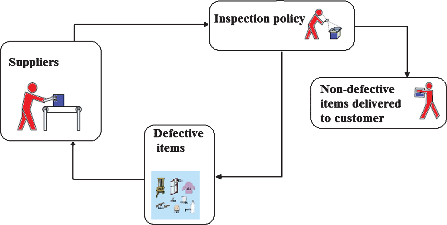
Behavior of buyer’s inspection policy.

4 Model formulation

Based on the above notations and assumptions, we develop a model for vendor-buyer integrated inventory system for defective items, with controllable lead time under permissible delay in payment to minimize the joint total expected cost.

4.1 Buyer’s expected total cost

The buyer places an order of Q units, therefore for expected cycle time of $\frac{Q}{D}$ , the expected ordering and lead time crashing cost per unit time can be given by $\frac{kD}{Q}$ and $\frac{DR (L)}{Q}$ . The expected net inventory level just before the arrival of a procurement quantity Q is only the safety stock τ = r - DL. Each shipment takes time $\frac{Q}{D}$ to be consumed by the buyer, thus $T = \frac{Q}{D}$ and during this time the buyer’s average inventory is Q/2. Also, the expected inventory over the cycle is $\frac{Q}{2} + τ σ \sqrt{L}$ . Therefore, the holding cost for the cycle stock per unit time is $\frac{c_{b} h_{b} Q}{2}$ . On the other hand, the safety stock $τ σ \sqrt{L}$ is held throughout the cycle. Therefore, according to credit policy, the interest is charged at the rate of I_p to this portion of stock by the vendor and the buyer must pay the holding cost for this portion of stock as well. Hence, the total cost for safety stock per unit time as sum of holding cost and interest charged, i.e. $(h_{b} + I_{p}) c_{b} τ σ \sqrt{L}$ .

According to our assumption, the credit period cannot be greater than the ordering time. Therefore, when the buyer’s permissible delay period expires on or before all inventories are depleted completely, the buyer can sell the items and earn interest with the rate of I_e until the end of the credit period M. Hence, the buyer’s interest earned per unit time is $\frac{D^{2} M^{2} {pI}_{e}}{2 Q}$ . In addition, the expected shortage B(r) is completely backordered in the previous cycle, which is cleared in the beginning of the current cycle, therefore, during the trade credit period the buyer earns an interest of $\frac{{DMpI}_{e} B (r)}{Q}$ per unit time. On the other hand, the buyer still has (Q - DM) units unsold at the end of the permissible delay. Hence, the buyer has a loan for the unpaid purchase cost of unsold units with the interest charge of I_p. Therefore, the opportunity interest cost per cycle time for the unsold items is obtained by $\frac{{(Q - DM)}^{2} c_{b} I_{p}}{2 Q}$ . The transportation cost is given by $\frac{FD}{Q}$ . The lead time crashing cost per order R(L), is assumed to be an exponential function of L.

Hence the total expected annual cost for the buyer consists of ordering cost, holding cost, safety stock cost, opportunity interest cost, lead time crashing cost, interest earned and the transportation cost is expressed as

$\begin{matrix} {EAC}_{b} (Q, L) \\ = \frac{kD}{Q} + \frac{{Qc}_{b} h_{b}}{2} + (h_{b} + I_{p}) c_{b} τ σ \sqrt{L} \\ + \frac{{(Q - DM)}^{2} c_{b} I_{p}}{2 Q} + \frac{DR (L)}{Q} \\ - \frac{D^{2} M^{2} {pI}_{e}}{2 Q} - \frac{{DMpI}_{e} B (r)}{Q} + \frac{FD}{Q} \end{matrix}$ (1)

4.2 Vendor’s expected total cost

Once the buyer orders a lot size of Q units, the vendor produces the items in a lot size of nQ units in each production cycle of length nQ/D with constant production rate P units per unit time, and the buyer will receive the supply in n lots each of size Q units. The first lot size of Q units is ready for shipment after time Q/P′ just after the start of the production. During the production period, nQ/P′, the vendor’s inventory is building up at a constant rate, and simultaneously supplies a lot of size Q units to the buyer on every Q/D units of time, thus T = Q/D. By assumption, the production processes are imperfect and the probability of an item to be defective is ɛ, and hence, the vendor’s effective annual production rate P′ = P (1 - ɛ). Since ɛ < 1 - D/P, (i, e . , P (1 - ɛ) > D) , Q/P′, the time taken to produce the first shipment of Q good quality items, is less than the cycle time T. Thus, a new production run will start at time T - Q/P′ after the last shipment of each production run. Hence, the vendors holding cost per year for non-defective items are obtained using the same approach as Uthayakumar and Priyan [35]. $\begin{matrix} {(nQ [\frac{Q}{P (1 - ɛ)} + (n - 1) T] - \frac{nQ (nQ)}{2 P (1 - ɛ)}) \\ - T (Q + 2 Q + \dots + (n - 1) Q)} \\ = {(nQ [\frac{Q}{P (1 - ɛ)} + (n - 1) T] \\ - \frac{n^{2} Q^{2}}{2 P (1 - ɛ)}) - \frac{Q}{D} (\frac{n (n - 1) Q}{2})} \\ = {\frac{{nQ}^{2}}{P (1 - ɛ)} [1 - \frac{n}{2}] + \frac{n (n - 1) Q^{2}}{2 D}} \end{matrix}$

At the beginning of each production period, there are zero defective items. After the period of production (which has duration of $\frac{nQ}{P (1 - ɛ)}$ ), the number of defective items produced is $\frac{nQ ɛ}{(1 - ɛ)}$ . Hence the holding cost for defective items and the good quality are $h_{v} {(\frac{nQ}{2} [\frac{ɛ}{1 - ɛ}]) (\frac{nQ}{P} [\frac{1}{1 - ɛ}])}$ and $h_{v} {\frac{{nQ}^{2}}{p (1 - ɛ)} [1 - \frac{n}{2}] + \frac{n (n - 1) Q^{2}}{2 D}}$ respectively. Since the production quantity for a vendor in a lot is nQ units, the set-up cost for the vendor is given by $\frac{k_{v} D}{nQ}$ . In addition, the buyer has a loan from a bank for the unsold products cost. Therefore, during the credit period of delayed payment, the vendor has an opportunity interest loss with annual rate I_v, by assumption I_v = I_e. Thus, the vendor’s opportunity interest loss per unit time is $\frac{I_{v} c_{b} MnQ}{nQ / D} = I_{v} c_{b} MD$ .

Hence, the vendor’s total expected annual cost comprising, the setup cost, inspection cost, the cost of defective items, holding cost and opportunity interest loss, can be expressed as

$\begin{matrix} {EAC}_{v} (Q, n) \\ = \frac{k_{v} D}{nQ} + c_{i} DE [\frac{1}{1 - ɛ}] + c_{d} DE [\frac{ɛ}{1 - ɛ}] \\ + h_{v} {\frac{QD}{P} [1 - \frac{n}{2}] E [\frac{1}{1 - ɛ}] \\ + \frac{(n - 1) Q}{2} + \frac{nQD}{2 P} E [\frac{ɛ}{{(1 - ɛ)}^{2}}]} \\ + I_{v} c_{b} MD \end{matrix}$ (2)

4.3 The integrated vendor-buyer inventory model

The expected total annual cost for the vendor-buyer integrated inventory system under permissible delay in payment is given by

$\begin{matrix} EAC (Q, L, n) \\ = {EAC}_{b} (Q, L) + {EAC}_{v} (Q, n) \\ EAC (Q, L, n) \\ = \frac{kD}{Q} + \frac{{Qc}_{b} h_{b}}{2} + (h_{b} + I_{p}) c_{b} τ σ \sqrt{L} \\ + \frac{{(Q - DM)}^{2} c_{b} I_{p}}{2 Q} + \frac{DR (L)}{Q} \\ - \frac{D^{2} M^{2} {pI}_{e}}{2 Q} - \frac{{DMpI}_{e} B (r)}{Q} + \frac{FD}{Q} \\ + \frac{k_{v} D}{nQ} + c_{i} DE [\frac{1}{1 - ɛ}] + c_{d} DE [\frac{ɛ}{1 - ɛ}] \\ + h_{v} {\frac{QD}{P} [1 - \frac{n}{2}] E [\frac{1}{1 - ɛ}] \\ + \frac{(n - 1) Q}{2} + \frac{nQD}{2 P} E [\frac{ɛ}{{(1 - ɛ)}^{2}}]} \\ + I_{v} c_{b} MD \end{matrix}$ (3) where E [x] denotes the expected value of x.

5 Solution procedure

5.1 Normal distribution model

The lead time demand X follows a normal probability distribution function with mean DL and standard deviation $σ \sqrt{L}$ and the reorder point, $r = DL + τ σ \sqrt{L}$ , where τ is the safety factor and σ, the standard deviation of the lead time demand. Therefore, the buyer’s expected demand shortages at the end of the cycle is given by $\begin{matrix} E {(X - r)}^{+} & = & B (r) = \int_{r}^{\infty} (x - r) f (x) dx \\ = & σ \sqrt{L} ψ (τ) \end{matrix}$ where ψ (τ) = φ (τ) - τ [1 - φ (τ)] > 0 and φ, φ are the standard normal p.d.f and cumulative distribution function respectively. In developing, the joint total expected cost of the system, the stockout cost term for the buyer is not considered. Normally, it is complicated to calculate the penalty costs associated with a shortage, as a stock-out event may include uncertain manipulates. As a result, authors like Jha and Shankar [27], Moon et. al. [36], Annadurai and Uthayakumar [37] assumes that buyer has set a target service level corresponding to proportion of demands to be satisfied directly from available stock. Hence, a service level constraint puts a limit on the proportion of demands not met from stock. From assumption (5), the actual proportion of demands not met from stock should not exceed the desired value of α. Hence, the Service level constraint can be expressed as

$\begin{matrix} \frac{Expected demand shortages at the end of the cycle for a given safety factor}{Quantity available for satisfying the demand per cycle} \\ \leq α \end{matrix}$ i.e., $\frac{B (r)}{Q} \leq α$

When the lead time demand follows normal distribution, service level constraint is given by $\frac{σ \sqrt{L} ψ (τ)}{Q} \leq α$

The total expected cost per unit time for the vendor-buyer integrated inventory system under permissible delay in payment is given by

$\begin{matrix} {EAC}^{N} (Q, L, n) \\ = \frac{D}{Q} {k + \frac{k_{v}}{n} + R (L) - {MpI}_{e} σ \sqrt{L} ψ (τ) + F \\ + \frac{{DM}^{2}}{2} (c_{b} I_{p} - {pI}_{e})} \\ + \frac{Q}{2} [(h_{b} + I_{p}) c_{b} \\ + h_{v} {\frac{D}{P} [2 - n] E [\frac{1}{1 - ɛ}] + (n - 1) \\ + \frac{nD}{P} E [\frac{ɛ}{{(1 - ɛ)}^{2}}]}] \\ + (h_{b} + I_{p}) c_{b} τ σ \sqrt{L} + c_{i} DE [\frac{1}{1 - ɛ}] \\ + c_{d} DE [\frac{ɛ}{1 - ɛ}] + {DMc}_{b} (I_{v} - I_{p}) \end{matrix}$ (4)

Now, the problem is to find the optimal lot size, lead time, setup cost and the total number of deliveries in a production cycle that minimize the joint total expected cost $\begin{matrix} min {EAC}^{N} (Q, L, n) \\ = \frac{D}{Q} {k + \frac{k_{v}}{n} + R (L) - {MpI}_{e} σ \sqrt{L} ψ (τ) + F \\ + \frac{{DM}^{2}}{2} (c_{b} I_{p} - {pI}_{e})} \\ + \frac{Q}{2} [(h_{b} + I_{p}) c_{b} \\ + h_{v} {\frac{D}{P} [2 - n] E [\frac{1}{1 - ɛ}] + (n - 1) \\ + \frac{nD}{P} E [\frac{ɛ}{{(1 - ɛ)}^{2}}]}] \\ + (h_{b} + I_{p}) c_{b} τ σ \sqrt{L} + c_{i} DE [\frac{1}{1 - ɛ}] \\ + c_{d} DE [\frac{ɛ}{1 - ɛ}] + {DMc}_{b} (I_{v} - I_{p}) \end{matrix}$ subject to $\frac{σ \sqrt{L} ψ (τ)}{Q} \leq α .$

In order to find the minimum total cost for this nonlinear programming problem, we temporarily relax the integer requirement on n, and then try to find the optimal solution of EAC^N (Q, L, n) with classical optimization technique by taking the first order partial derivatives of EAC^N (Q, L, n) with respect to Q.

For fixed Q and L ∈ [L_b, L₀] , EAC^N (Q, L, n) can be proved to be a convex function of n.

Proposition 1. For fixed Q and L ∈ [L_b, L₀] , EAC^N (Q, L, n) is convex in n.

Proof. Taking the first and second partial derivatives of EAC^N (Q, L, n) with respect to n, we have $\begin{matrix} \frac{\partial {EAC}^{N} (Q, L, n)}{\partial n} \\ = - \frac{{Dk}_{v}}{{Qn}^{2}} + \frac{{Qh}_{v}}{2} {\frac{- D}{P} E [\frac{1}{1 - ɛ}] \\ + 1 + \frac{D}{P} E [\frac{ɛ}{{(1 - ɛ)}^{2}}]} \\ \frac{\partial^{2} {EAC}^{N} (Q, L, n)}{\partial n^{2}} = \frac{2 {Dk}_{v}}{{Qn}^{3}} > 0 . \end{matrix}$

Therefore, for fixed Q and L ∈ [L_b, L₀] , EAC^N (Q, L, n) is convex in n.

Now, for fixed n, we take the first partial derivatives of EAC^N (Q, L, n) with respect to Q. $\begin{matrix} \frac{\partial {EAC}^{N} (Q, L, n)}{\partial Q} \\ = - \frac{D}{Q^{2}} [k + \frac{k_{v}}{n} + R (L) - {MpI}_{e} σ \sqrt{L} ψ (τ) + F \\ + \frac{{DM}^{2}}{2} (c_{b} I_{p} - {pI}_{e})] \\ + \frac{1}{2} [(h_{b} + I_{p}) c_{b} \\ + h_{v} {\frac{D}{P} [2 - n] E [\frac{1}{1 - ɛ}] + (n - 1) \\ + \frac{nD}{P} E [\frac{ɛ}{{(1 - ɛ)}^{2}}]}] \end{matrix}$

By setting the above equation equal to zero, for a given value of L ∈ [L_b, L₀], we obtain

$Q = \sqrt{\frac{2 D [k + \frac{k_{v}}{n} + R (L) - {MpI}_{e} σ \sqrt{L} ψ (τ) + F + \frac{{DM}^{2}}{2} (c_{b} I_{p} - {pI}_{e})]}{(h_{b} + I_{p}) c_{b} + h_{v} {\frac{D}{P} [2 - n] E [\frac{1}{1 - ɛ}] + (n - 1) + \frac{nD}{P} E [\frac{ɛ}{{(1 - ɛ)}^{2}}]}}}$ (5)

Theoretically, for fixed n and L ∈ [L_b, L₀], we can obtain the optimal value of Q. Moreover, for fixed n, the Hessian matrix of EAC^N (Q, L, n) is positive definite. (See Appendix A)

Computational Algorithm 1

Step 1. Set n = 1.

Step 2. For each L ∈ [L_b, L₀], perform steps (2.1) to (2.3).

Step (2.1). Determine the value of Q using Equation (5).

Step (2.2). Let $\bar{Q} = max {Q, (σ / α) \sqrt{L} ψ (τ)}$ .

Step (2.3). Compute the corresponding ${EAC}^{N} (\bar{Q}, L, n)$ using Equation (4).

Step 3. Find $min_{L \in [L_{b}, L_{0}]} {EAC}^{N} (\bar{Q}, L, n)$ . Let ${EAC}^{N} (Q_{(n)}^{*}, L_{(n)}^{*}, n) = min_{L \in [L_{b}, L_{0}]} {EAC}^{N} (\bar{Q}, L, n)$ , then $(Q_{(n)}^{*}, L_{(n)}^{*}, n)$ is the optimal solution for fixed n.

Step 4. Set n = n + 1, repeat steps 2 and 3 and find ${EAC}^{N} (Q_{(n)}^{*}, L_{(n)}^{*}, n)$ .

Step 5. If ${EAC}^{N} (Q_{(n)}^{*}, L_{(n)}^{*}, n) \leq {EAC}^{N} (Q_{(n - 1)}^{*}, L_{(n - 1)}^{*}, n - 1)$ , then go to step 4, otherwise go to step 6.

Step 6. Set ${EAC}^{N} (Q^{*}, L^{*}, n^{*}) = {EAC}^{N} (Q_{(n - 1)}^{*}, L_{(n - 1)}^{*}, n - 1)$ , then (Q^*, L^*, n^*) is the set of optimal solution and EAC^N (Q^*, L^*, n^*) is the minimum joint total expected cost.

5.2 Distribution free model

In the previous section, a model is developed under the assumption that the lead time demand follows a normal distribution. Practically, it is seen that the information about the probability distribution of the lead time is limited. Hence in this section, we assume that the density function F of lead time demand X belongs to the class of density functions with a known finite mean DL and standard deviation $σ \sqrt{L}$ and we

try to use a mini-max distribution free procedure to solve this problem. ${Min}_{Q, L, n} {Max}_{\overset{ˇ}{F} \in Ω} {EAC}^{U} (Q, L, n)$ (6)

To solve our problem, we apply the following proposition which was asserted by Gallego and Moon [38], Annadurai and Uthayakumar [39].

Proposition 2. For any $\overset{ˇ}{F} \in Ω$ ,

$\begin{matrix} E {(X - r)}^{+} \\ \leq \frac{1}{2} {\sqrt{σ^{2} L + {(r - DL)}^{2}} - (r - DL)} \end{matrix}$ (7)

Substituting $r = DL + τ σ \sqrt{L}$ into (7), we obtain the following inequality $E {(X - r)}^{+} \leq \frac{1}{2} {σ \sqrt{L} (\sqrt{1 + τ^{2}} - τ)}$ (8)

Now using (3) and inequality (8), (6) reduces to minimize $\begin{matrix} {EAC}^{U} (Q, L, n) = \frac{D}{Q} {k + \frac{k_{v}}{n} + R (L) \\ - {MpI}_{e} σ \sqrt{L} (\sqrt{1 + τ^{2}} - τ) \\ + F + \frac{{DM}^{2}}{2} (c_{b} I_{p} - {pI}_{e})} \\ + \frac{Q}{2} [(h_{b} + I_{p}) c_{b} \\ + h_{v} {\frac{D}{P} [2 - n] E [\frac{1}{1 - ɛ}] + (n - 1) \\ + \frac{nD}{P} E [\frac{ɛ}{{(1 - ɛ)}^{2}}]}] + (h_{b} + I_{p}) c_{b} τ σ \sqrt{L} \\ + c_{i} DE [\frac{1}{1 - ɛ}] + c_{d} DE [\frac{ɛ}{1 - ɛ}] \\ + {DMc}_{b} (I_{v} - I_{p}) \end{matrix}$ subject to $\frac{σ \sqrt{L} ψ (τ)}{Q} \leq α$ (9) where EAC^U (Q, L, n) is the least upper bound of EAC (Q, L, n).

As on before, for fixed n, it can be verified that the values of Q, L and n satisfy the second order sufficient conditions and we can show that EAC^U (Q, L, n) is a convex in Q. Hence, to find the optimal value, we take the partial derivative of EAC^U (Q, L, n) with respect to Q. $\begin{matrix} \frac{\partial {EAC}^{U} (Q, L, n)}{\partial Q} = - \frac{D}{Q^{2}} [k + \frac{k_{v}}{n} + R (L) \\ - {MpI}_{e} σ \sqrt{L} (\sqrt{1 + τ^{2}} - τ) + F \\ + \frac{{DM}^{2}}{2} (c_{b} I_{p} - {pI}_{e})] \\ + \frac{1}{2} [(h_{b} + I_{p}) c_{b} \\ + h_{v} {\frac{D}{P} [2 - n] E [\frac{1}{1 - ɛ}] + (n - 1) \\ + \frac{nD}{P} E [\frac{ɛ}{{(1 - ɛ)}^{2}}]}] \end{matrix}$

By setting the above equation equal to zero, for a given value of L ∈ (L_b, L₀), we obtain

$Q = \sqrt{\frac{2 D [k + \frac{k_{v}}{n} + R (L) - {MpI}_{e} σ \sqrt{L} (\sqrt{1 + τ^{2}} - τ) + F + \frac{{DM}^{2}}{2} (c_{b} I_{p} - {pI}_{e})]}{(h_{b} + I_{p}) c_{b} + h_{v} {\frac{D}{P} [2 - n] E [\frac{1}{1 - ɛ}] + (n - 1) + \frac{nD}{P} E [\frac{ɛ}{{(1 - ɛ)}^{2}}]}}}$ (10)

Theoretically, for fixed n and L ∈ [L_b, L₀], we can obtain the optimal value of Q. Moreover, for fixed n, the Hessian matrix of EAC^U (Q, L, n) is positive definite. (See Appendix B)

Computational Algorithm 2

Step 1. Set n = 1.

Step 2. For each L ∈ [L_b, L₀], perform steps (2.1) to (2.3).

Step (2.1). Determine the value of Q using Equation (10).

Step (2.2). Let $\bar{Q} = max {Q, (σ / α) \sqrt{L} ψ (τ)}$ .

Step (2.3). Compute the corresponding ${EAC}^{U} (\bar{Q}, L, n)$ using Equation (9).

Step 3. Find $min_{L \in [L_{b}, L_{0}]} {EAC}^{U} (\bar{Q}, L, n)$ .

Let ${EAC}^{U} (Q_{(n)}^{*}, L_{(n)}^{*}, n) = min_{L \in [L_{b}, L_{0}]} {EAC}^{U} (\bar{Q}, L, n)$ , then $(Q_{(n)}^{*}, L_{(n)}^{*}, n)$ is the optimal solution for fixed n.

Step 4. Set n = n + 1, repeat steps 2 and 3 and find ${EAC}^{U} (Q_{(n)}^{*}, L_{(n)}^{*}, n)$ .

Step 5. If ${EAC}^{U} (Q_{(n)}^{*}, L_{(n)}^{*}, n) \leq {EAC}^{U} (Q_{(n - 1)}^{*}, L_{(n - 1)}^{*}, n - 1)$ , then go to step 4, otherwise go to step 6.

Step 6. Set $\begin{matrix} {EAC}^{U} (Q^{*}, L^{*}, n^{*}) \\ = {EAC}^{U} (Q_{(n - 1)}^{*}, L_{(n - 1)}^{*}, n - 1) \end{matrix}$ then (Q^*, L^*, n^*) is the set of optimal solution and EAC^U (Q^*, L^*, n^*) is the minimum joint total expected cost.

6 Numerical examples

In this section we illustrate the proposed model with numerical examples.

Example 1. Consider an inventory system with the following characteristics:

D = 800 units/year, P = 1600 units/year, k = $200/order, k_v = $400/setup, h_b = $4/unit/year, h_v = $2/unit/year, F = $25/delivery, c_b = $10/unit, p = $30/ unit, τ= 0.75 (the value of ψ (τ) can be found directly from the standard normal table and is equal to 0.1311), σ= 15units per week, where 1 year = 52 weeks, the service level (1 - α) = 0.985, c_i = $0.5/unit, c_d = $25/unit, M = 0.0833 year, I_v = 0.02 $/year, I_p = 0.06 $/year, I_e = 0.02 $/year, crashing cost $R (L) = {\begin{matrix} 0 & if L = 10 \\ e^{C / L} & if 1 \leq L < 10 \end{matrix}$ where C = 5.

If the defective percentage follows a uniform distribution with $f (ɛ) = {\begin{matrix} \frac{1}{β}, & 0, \leq ε \leq β \\ 0, & otherwise \end{matrix}$ then $\begin{matrix} E [\frac{1}{1 - ɛ}] & = & \int_{0}^{β} \frac{1}{1 - ɛ} f (ɛ) d ɛ = - \frac{\ln (1 - β)}{β} . \\ E [\frac{ɛ}{1 - ɛ}] & = & E [\frac{1}{1 - ɛ} - 1] = E [\frac{1}{1 - ɛ}] - 1 \\ = & - \frac{\ln (1 - β)}{β} - 1 . \\ E [\frac{1}{{(1 - ɛ)}^{2}}] & = & \frac{1}{1 - β}, and \\ E [\frac{ɛ}{{(1 - ɛ)}^{2}}] & = & E [\frac{1}{{(1 - ɛ)}^{2}} - \frac{1}{1 - ɛ}] \\ = & \frac{1}{1 - β} + \frac{\ln (1 - β)}{β} . \end{matrix}$

Let β = 0.02. The optimal values of Q, L and n are obtained using the computational algorithm 1 and the values are given by L^* = 2 weeks, Q^* = 101.56 units, number of deliveries n^* = 3 and the corresponding expected total cost is EAC^N (Q^*, L^*, n^*) = $5794.50.

Example 2. Consider the same data as in Example 1, except that the probability distribution of the lead time demand is unknown (Distribution free approach). Using computational Algorithm 2, we obtain the optimal values and the values are L^* = 2 weeks, Q^* = 141.44 units, number of deliveries n^* = 3 and the corresponding expected total cost EAC^U (Q^*, L^*, n^*) = $6588.40.

7 Sensitivity analysis

The change in the values of parameters may happen due to uncertainties in any decision-making situation. In order to examine the implications of these changes, the sensitivity analysis will be of great help in decision making. Using the numerical example, given in the previous section, the sensitivity analysis of various parameters has been done. The results of sensitivity analysis are summarized in Tables 1 to 10 and Figs. 2–10.

When the demand rate D increases, the optimal ordering quantity Q^* and the total expected annual cost EAC (Q^*, L^*, n^*) increases in both the models.

Increasing the vendor’s production rate P results in a decrease in the ordering quantity Q^* and an increase in the total expected annual cost EAC (Q^*, L^*, n^*) when the distribution of the lead time demand is known. Whereas, there is an increase in the ordering quantity Q^* and the total expected cost EAC (Q^*, L^*, n^*) when the distribution is unknown.

When there is an increase in the buyer’s ordering cost k, there is an increase in the ordering quantity Q^* and the total expected annual cost EAC (Q^*, L^*, n^*) in both the models.

There is a positive change in the total expected cost EAC (Q^*, L^*, n^*) in both the models when the vendor’s setup cost k_v increases.

Increasing vendor’s holding cost h_v results in a marginal change in the ordering quantity Q^*. The total expected cost EAC (Q^*, L^*, n^*) increases with respect to an increase in h_v in both the models.

There is a decrease in the optimal ordering quantity Q^* and an increase in the optimal total cost in the normal distribution model, when the buyer’s holding cost rate h_b increases. When the distribution of lead time demand is unknown, there is an increase in both the ordering quantity Q^* and the total expected cost EAC (Q^*, L^*, n^*).

When α decreases, the optimal order quantity Q^* and the total expected cost EAC (Q^*, L^*, n^*) increases in both the models.

There is a positive change in optimal order quantity Q^* and a negative change in the total expected cost EAC (Q^*, L^*, n^*) with respect to M in both the models.

Fig.2

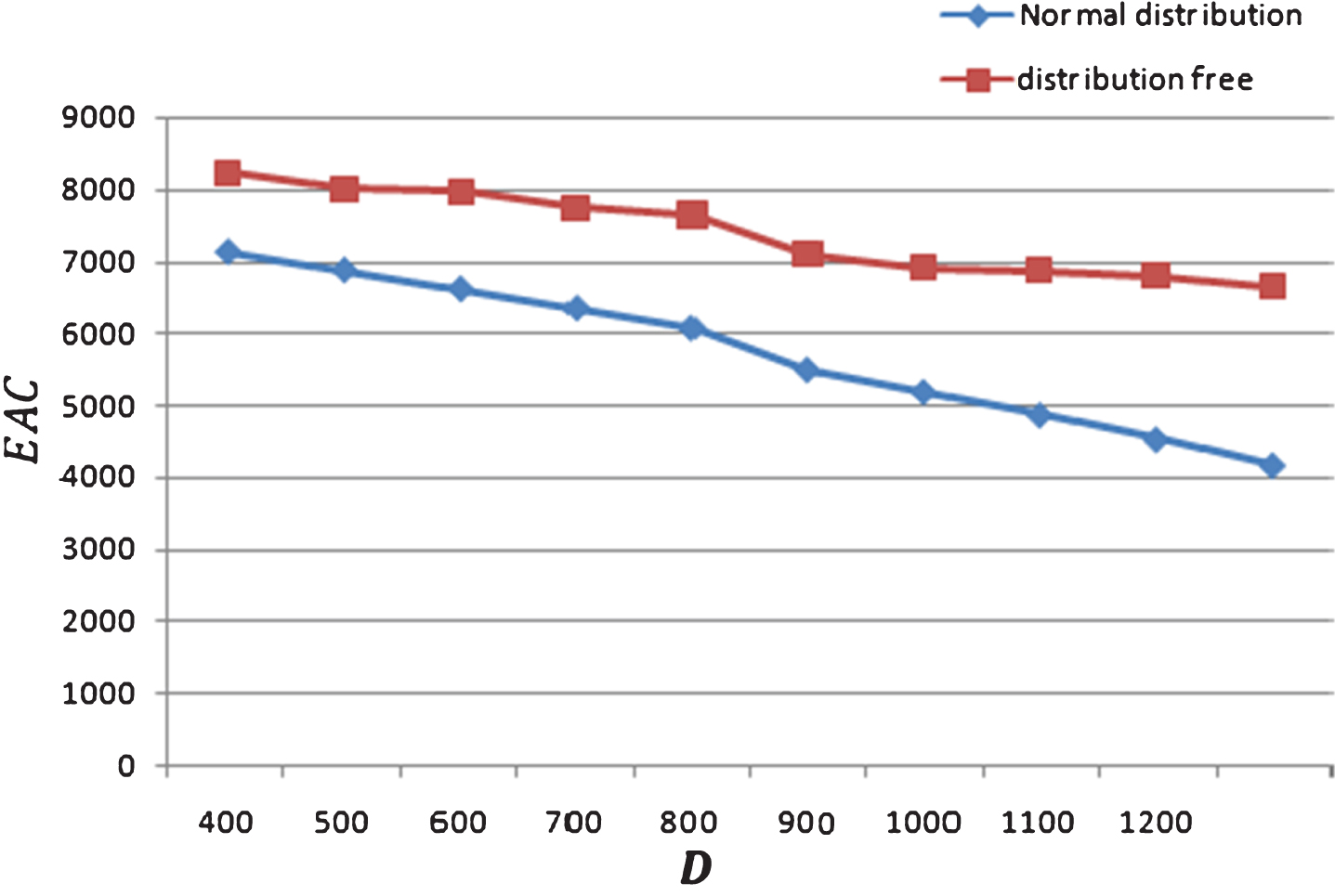
Change of demand rate (D) on EAC.

Fig.3

Change of production rate (P) on EAC.

Fig.4

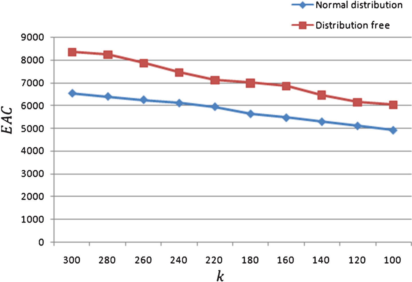
Change of ordering cost (k) on EAC.

Fig.5

Change of setup cost (k_v) on EAC.

Fig.6

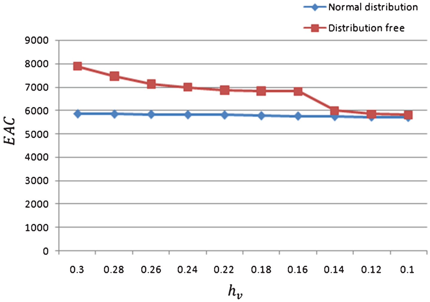
Change of vendor’s holding cost (h_v) on EAC.

Fig.7

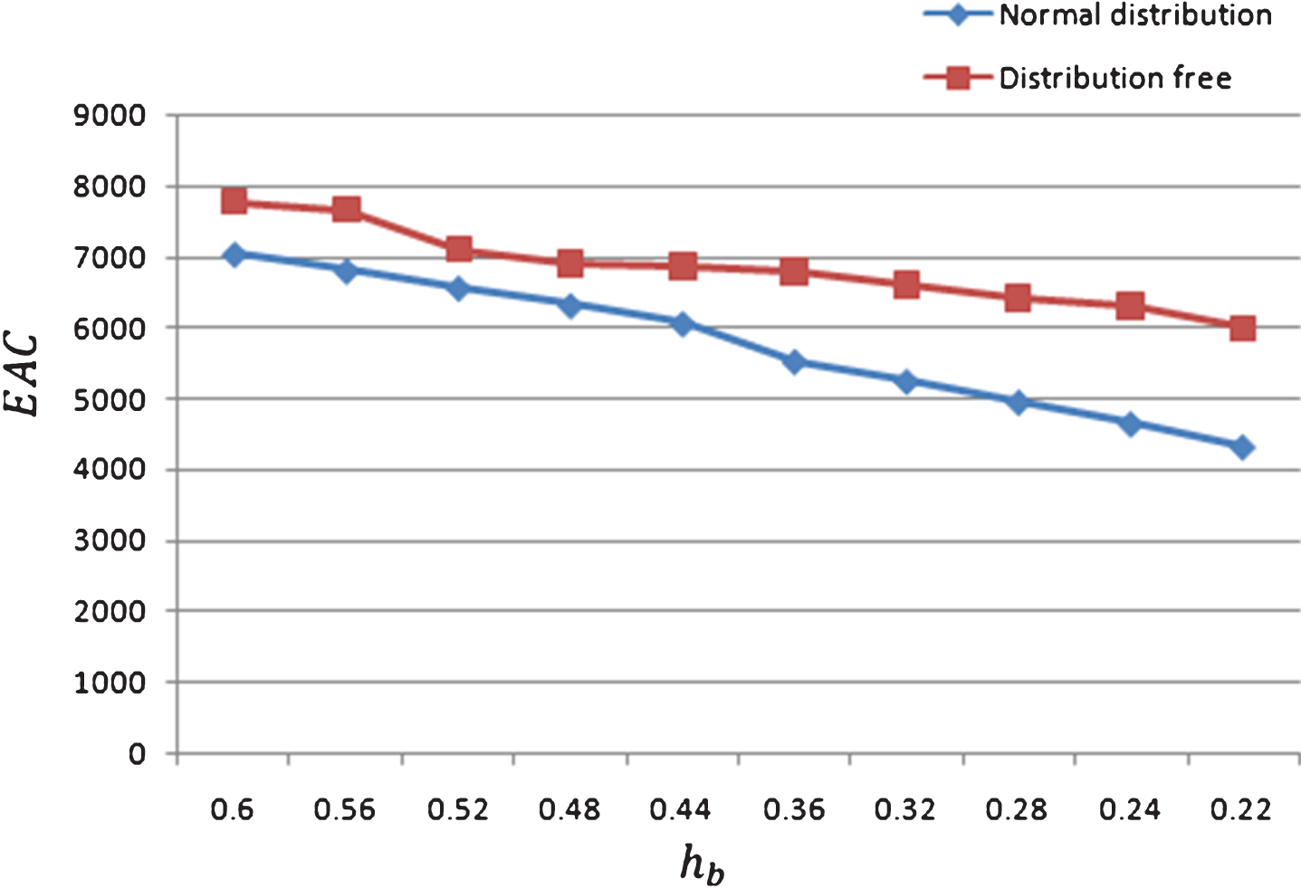
Change of buyer’s holding cost (h_b) on EAC.

Fig.8

Change of (β) on EAC.

Fig.9

Change of freight rate (F) on EAC.

Fig.10

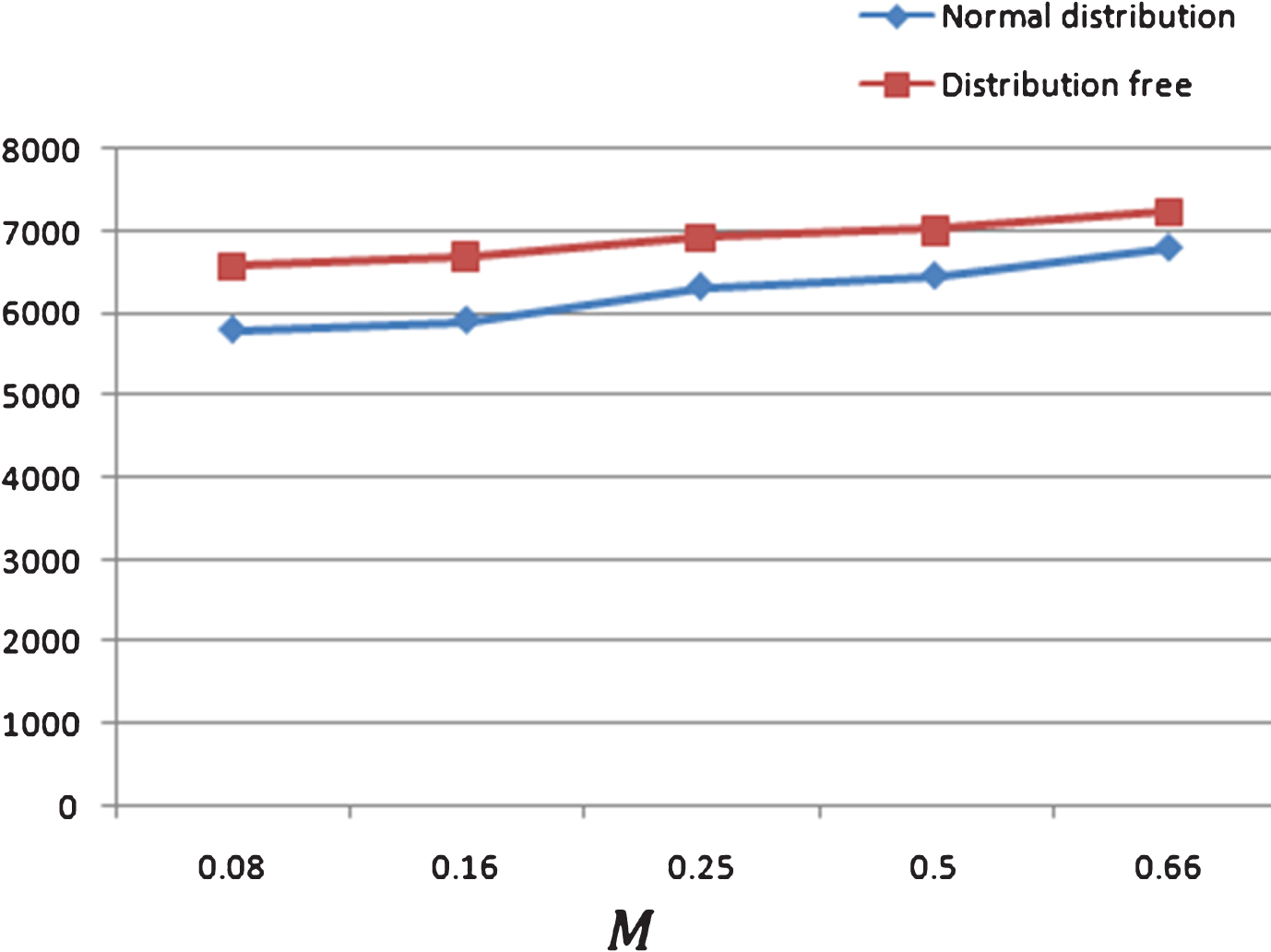
Change of freight rate (M) on EAC.

Table 1

Effect of change in D on the optimal solution

D	Normal Distribution Model				Distribution Free Model				EVAI
	n ^*	L ^*	Q ^*	EAC^N (Q^, L^, n^*)	n ^*	L ^*	Q ^*	EAC^U (Q^, L^, n^*)
50%	3	2	131.26	7141.00	3	2	156.78	8231.98	1090.98
30%	3	2	119.15	6626.50	3	2	139.76	7960.34	1333.84
10%	3	2	107.66	6081.10	3	2	117.50	7651.09	1569.99
–10%	3	2	95.34	5497.50	3	2	108.11	7102.34	1604.84
–30%	3	2	82.37	4865.20	3	2	98.39	6860.00	1994.80
–50%	3	2	68.24	4161.90	3	2	97.01	6650.45	2488.55

Table 2

Effect of change in P on the optimal solution

P	Normal Distribution Model				Distribution Free Model				EVAI
	n ^*	L ^*	Q ^*	EAC^N (Q^, L^, n^*)	n ^*	L ^*	Q ^*	EAC^U (Q^, L^, n^*)
50%	3	2	101.55	5838.80	3	2	134.98	7345.98	1510.18
30%	3	2	101.56	5825.90	3	2	127.80	6783.23	957.33
10%	3	2	101.71	5807.40	3	2	126.32	6201.10	393.70
–10%	3	2	101.55	5777.80	3	2	118.71	6111.23	333.43
–30%	3	2	102.08	5723.10	3	2	115.11	5991.34	268.24
–50%	3	2	104.30	5619.40	3	2	116.12	5820.56	201.16

Table 3

Effect of change in k on the optimal solution

k	Normal Distribution Model				Distribution Free Model				EVAI
	n ^*	L ^*	Q ^*	EAC^N (Q^, L^, n^*)	n ^*	L ^*	Q ^*	EAC^U (Q^, L^, n^*)
50%	3	2	117.45	6524.80	3	2	131.26	8349.10	1824.30
30%	3	2	111.45	6245.20	3	2	119.15	7876.10	1630.90
10%	3	2	104.94	5949.40	3	2	112.66	7121.98	1172.59
–10%	3	2	98.09	5634.30	3	2	112.34	6987.34	1353.04
–30%	3	2	90.80	5295.50	3	2	101.37	6456.09	1160.59
–50%	3	2	82.80	4926.60	3	2	99.24	6030.87	1104.27

Table 4

Effect of change in k_v on the optimal solution

k_v	Normal Distribution Model				Distribution Free Model				EVAI
	n ^*	L ^*	Q ^*	EAC^N (Q^, L^, n^*)	n ^*	L ^*	Q ^*	EAC^U (Q^, L^, n^*)
50%	3	2	101.60	5855.90	3	2	112.12	8342.12	2486.22
30%	3	2	101.57	5832.80	3	2	109.47	7561.87	1729.07
10%	3	2	101.64	5807.90	3	2	108.12	7432.19	1624.29
–10%	3	2	101.67	5780.50	3	2	108.00	7238.09	1457.59
–30%	3	2	101.62	5749.70	3	2	106.89	7198.52	1448.82
–50%	3	2	101.67	5714.50	3	2	105.78	7123.56	1409.06

Table 5

Effect of change in h_v on the optimal solution

h_v	Normal Distribution Model				Distribution Free Model				EVAI
	n ^*	L ^*	Q ^*	EAC^N (Q^, L^, n^*)	n ^*	L ^*	Q ^*	EAC^U (Q^, L^, n^*)
50%	3	2	101.46	5856.40	3	2	111.76	7876.10	2019.70
30%	3	2	101.66	5833.10	3	2	111.20	7121.98	1288.88
10%	3	2	101.70	5808.00	3	2	109.78	6856.23	1048.23
–10%	3	2	101.67	5780.40	3	2	109.32	6823.12	1042.72
–30%	3	2	101.67	5749.70	3	2	103.21	5987.01	237.31
–50%	3	2	101.23	5716.20	3	2	101.21	5811.66	95.46

Table 6

Effect of change in h_b on the optimal solution

h_b	Normal Distribution Model				Distribution Free Model				EVAI
	n ^*	L ^*	Q ^*	EAC^N (Q^, L^, n^*)	n ^*	L ^*	Q ^*	EAC^U (Q^, L^, n^*)
50%	3	2	84.77	7037.40	3	2	101.57	7756.10	718.70
30%	3	2	90.53	6559.80	3	2	101.64	7102.34	542.54
10%	3	2	97.46	6057.10	3	2	101.56	6860.00	802.90
–10%	3	2	106.22	5523.10	3	2	101.62	6790.01	1266.91
–30%	3	2	118.10	4948.00	3	2	98.17	6419.34	1471.34
–50%	3	2	134.98	4316.40	3	2	91.01	6011.88	1695.48

Also, we examine the performance of the distribution free approach against the normal distribution model.

The optimal solution of the normal distribution model and the distribution free model are EAC^N (Q^*, L^*, n^*) and EAC^U (Q^*, L^*, n^*) respectively. The added cost obtained by utilizing the mini-max distribution free procedure instead of the normal distribution model is EAC^N (Q^*, L^*, n^*) - EAC^U (Q^*, L^*, n^*). This is the largest amount that we would be willing to pay for the knowledge of the probability distribution of the demand and this quantity can be regarded as the expected value of additional information (EVAI) and is given in the tables.

8 Managerial implications

Using the sensitivity analysis carried, we infer the following managerial insights:

When there is an increase in Freight cost F, the total expected annual cost and the lot size Q^* increases when the lead time demand follows normal distribution. But, in the distribution free model there is a positive change in the optimal order quantity Q^* and a negative change in the expected annual cost. From this we infer that, when the transportation cost is high, the retailer should take necessary steps to order large quantity so that the total expected cost is minimized, when the information about the lead time demand is known and it follows normal distribution. Further, we observe that, increase in service level results in an increase in the total expected cost and the optimal order quantity, that is, the buyer could provide improved customer service and gain goodwill of the customer by ordering larger quantity. Increase in the ordering cost k, results in considerable increase in the total expected cost and the order quantity without affecting the lead time. From inventory point of view, the retailer should order more quantity per order when the ordering cost is high. The retailer may take necessary steps to reduce the ordering cost per order by some capital investment. When the demand rate is high, the vendor may lose production efficiency which results in high total cost. Therefore the design of production capacity is important in controlling production cost. Also, the benefit of the integrated model is more significant for high values of demand rate. From Table 7, it can be observed that, increase in the defective percentage ɛ (note that ɛ is uniformly distributed between 0 and β) causes the production quantity to decrease. For higher values of β, the total expected cost is also high. From managerial view point, it is advised that the supplier should find some measure to decrease the defective rate. That is, the supplier should entertain quality production to reduce the total expected cost of the supply chain. The service level constraint (which refers to the performance metrics used to measure the customer service in the supply chain) is an important tool used in industry like software development, automobile, etc. Our research results shows that these industries can provide improved customer service and gain goodwill of the customers by ordering large quantity. The design of the production capacity is also vital. The failure rate of an electronic device in the auto industry affects the entire supply chain. Our analysis shows that some effective measure should be taken to decrease the defective rate and to reduce the total expected cost of the integrated system so that customer satisfaction may be achieved.

Table 7
Effect of change in β on the optimal solution

β Normal Distribution Model Distribution Free Model EVAI

n ^* L ^* Q ^* EAC^N (Q^, L^, n^) n ^ L ^* Q ^* EAC^U (Q^, L^, n^*)

0.04 3 2 101.56 6042.60 3 2 101.43 6048.80 6.20

0.06 3 2 101.56 6304.10 3 2 101.43 6310.30 6.20

0.08 3 2 101.55 6573.10 3 2 101.42 6579.30 6.20

0.10 3 2 101.54 6850.20 3 2 101.42 6856.10 6.10

β	Normal Distribution Model	Distribution Free Model	EVAI
0.04	3	2	101.56	6042.60	3	2	101.43	6048.80	6.20
0.06	3	2	101.56	6304.10	3	2	101.43	6310.30	6.20
0.08	3	2	101.55	6573.10	3	2	101.42	6579.30	6.20
0.10	3	2	101.54	6850.20	3	2	101.42	6856.10	6.10

Table 8

Effect of change in F on the optimal solution

F	Normal Distribution Model				Distribution Free Model				EVAI
	n ^*	L ^*	Q ^*	EAC^N (Q^, L^, n^*)	n ^*	L ^*	Q ^*	EAC^U (Q^, L^, n^*)
30	3	2	102.37	5833.70	3	2	110.23	6798.65	964.95
40	3	2	104.16	5911.20	3	2	117.12	6665.98	754.78
50	3	2	105.73	5987.40	3	2	121.98	6548.54	561.14
100	3	2	113.66	6351.80	3	2	130.54	6456.21	104.41
150	3	2	121.15	6392.50	3	2	135.09	6421.70	29.20

Table 9

Effect of change in M on the optimal solution

M	Normal Distribution Model				Distribution Free Model				EVAI
	n ^*	L ^*	Q ^*	EAC^N (Q^, L^, n^*)	n ^*	L ^*	Q ^*	EAC^U (Q^, L^, n^*)
0.08	3	2	101.56	5794.50	3	2	140.44	6588.40	793.90
0.16	3	2	113.01	5578.01	3	2	159.32	6504.74	926.73
0.25	3	2	125.26	5501.12	3	2	162.45	6485.15	984.03
0.50	3	2	142.73	5481.89	3	2	171.10	6449.42	967.53
0.66	3	2	152.66	5350.48	3	2	184.23	6301.58	951.10

Table 10

Effect of change in α on the optimal solution

Service Level (1 - α)	α	Normal Distribution Model				Distribution Free Model				EVAI
	n ^*	L ^*	Q ^*	EAC^N (Q^, L^, n^*)	n ^*	L ^*	Q ^*	EAC^U (Q^, L^, n^*)
0.975	0.025	3	2	90.71	5592.55	3	2	108.47	6491.45	898.90
0.980	0.020	3	2	95.48	5610.19	3	2	129.12	6504.71	894.52
0.985	0.015	3	2	101.56	5794.50	3	2	140.44	6588.40	793.90
0.990	0.010	2	2	111.45	5806.76	3	2	174.80	6674.23	867.47
0.995	0.005	2	2	128.64	6001.80	3	2	187.37	6797.18	795.38

9 Conclusion and future research

In this article, we consider the single-vendor single-buyer integrated inventory problem for defective items. Lead time demand is assumed to follow normal distribution that is suitable to certain environment. There are situations where the information about the lead time demand is limited. Distribution free approach developed in this article will be appropriate to such situations. In our study, we minimize the joint total expected cost per unit time of the vendor and buyer by simultaneously optimizing the order quantity, lead time and the number of lots delivered from the vendor to the buyer in a production cycle with service level constraint.

In day-to-day life, trade credit financing becomes an essential tool to improve sales and gain profits in any industry. This plays a vital role in the financial management of inventory control for many organizations. To suit to this type of circumstances, a decision making integrated inventory model is presented, where trade credit is offered by the supplier to encourage the retailers to buyer more products and improve sales. From the analysis carried, we observe that, when the length of the credit period is longer, the total cost of the integrated system is reduced. Therefore from managerial point of view, trade credit policy may be used to a maximum extent so that both the buyer and the vendor are mutually benefited. To ensure the quality of the products, an inspection policy is used by the supplier and the defective items are removed from the lot and only non-defective items are supplied to the buyer. Necessary steps may be taken by the buyer to order large quantity to provide better customer service. The proposed model is well suitable to industries producing mobile phones, computers, textiles, healthcare products, automobiles etc. In future, this work may be extended by considering inflation rate, different types of demand, price discount and setup cost reduction. The fuzzy nature of the lead time demand may be considered as future work.

Footnotes

Appendix

References

Geetha

K.V

and Udayakumar

, Optimal replenishment policy for deteriorating items with time sensitive demand under trade credit financing, Amer J of Math and Manag Sci 34(2) (2015), 197–212.

Chung

C.J.

, An easy method to derive the integrated vendor buyer production inventory model with backordering using cost-difference rate comparison approach, Math and Comp Mod 57 (2013), 632–640.

Hill

R.M.

, The single-vendor single-buyer integrated production inventory model with a generalised policy, Euro J of Oper Res 97 (1997), 493–499.

Sarmah

S.P.

, Acharya

and Goyal

S.K.

, Buyer vendor coordination models in supply chain management, Euro J of Oper Res 175 (2006), 1–15.

Yao

, Philip Eversb

, and Dresner

M.E.

, Supply chain integration in vendor-managed inventory, Deci Supp Syst 43 (2007), 663–674.

Zhang

, Liang

, Yu

and Yu

, An integrated vendor-managed inventory model for a two-echelon system with order cost reduction, Int J of Pro Econ 109 (2007), 241–253.

Huang

C.K.

, Cheng

T.L.

, Tsai

D.M.

and Wu

J.C.

, An integrated vendor buyer inventory model with order processing cost reduction, J of Interdis Math 10 (4) (2007), 559–567.

Rau

, and Ouyang

B.C

, An optimal batch size for integrated production inventory policy in a supply chain, Euro J of Oper Res 185 (2008), 619–634.

Lin

Y.J.

and Ho

C.H.

, Integrated inventory model with quantity discount and price-sensitive demand, TOP 19 (2011), 177–188.

10.

Jaggi

C.K.

, Sharma

and Tiwari

, Credit financing in economic ordering policies for non-instantaneous deteriorating items with price dependent demand under permissible delay in payments, Int J of Ind Eng Comp 6 (2015), 481–502.

11.

Geetha

K.V.

and Udayakumar

, Optimal lot sizing policy for non instantaneous deteriorating items with price and advertisement dependent demand under partial backlogging, Int J of App and Comp Math 2(2) (2015), 171–193.

12.

Baten

M.A.

and Khalid

, Optimal production cycle time for inventory model with linear time dependent exponential distributed deterioration, J of Int and Fuzzy Sys 30 (2016), 1243–1248.

13.

Baten

M.A.

and Khalid

, Optimal control of a continuous review inventory system with gamma distributed deterioration, J of Int and Fuzzy Sys 27 (2014), 2937–2948.

14.

Udayakumar

and Geetha

K.V.

, Optimal replenishment policy for items with inflation rate and time dependent demand with salvage value, Art Int Sys and Machine Learn 6 (5) (2014), 193–197.

15.

Udayakumar

and Geetha

K.V.

, Economic ordering policy for single item inventory model over finite time horizon, Int J of Sys Assu Engg and Manag (2016). doi: 10.1007/s13198-016-0516-1

16.

Udayakumar

and Geetha

K.V.

, An EOQ model for non-instantaneous deteriorating items with two levels of storage under trade credit policy, J of Indus Engg Int (2017). doi:10.1007/s40092-017-0228-4

17.

Huang

C.K.

, An integrated inventory model for supplier and retailer with detective items, J of Inf and Opt Sci 22 (3) (2001), 509–519.

18.

Goyal

S.K.

, Huang

C.K.

and Chen

K.C.

, A simple integrated production policy of an imperfect item for vendor and buyer, Prod Plan and Con: The Mana of Oper 14 (7) (2003), 596–602.

19.

Sana

S.S.

, A production-inventory model of imperfect quality products in a three-layer supply chain, Deci Supp Syst 50 (2015), 539–547.

20.

Lin

H.J.

and Lin

Y.J.

, Supply chain coordination with defective items and quantity discount, Int J of Sys Sci 45 (12) (2013), 2529–2538.

21.

Ouyang

L.Y.

, Chen

L.Y.

and Yang

C.T.

, Impacts of collaborative investment and inspection policies on the integrated inventory model with defective items, Int J of Prod Res 51 (19) (2013), 5789–5802.

22.

Hsu

J.T.

and Hsu

L.F.

, An integrated vendor buyer cooperative inventory model in an imperfect production process with shortage backordering, Int J Adv Manag Tech 19 (2013), 493–505.

23.

Goyal

S.K.

, A note on: On controlling the controllable lead time component in the integrated inventory models, Int J of Pro Res 41 (12) (2003), 2873–2875.

24.

Ouyang

L.Y.

, Wu

K.S.

and Ho

C.H.

, Integrated vendor buyer cooperative models with stochastic demand in controllable lead time, Int J of Pro Econ 92 (2004), 255–266.

25.

Ouyang

L.Y.

, Wu

K.S.

and Ho

C.H.

, An integrated vendor buyer inventory model with quality improvement and lead time reduction, Int J of Pro Econ 108 (2007), 349–358.

26.

Ben-Daya

and Hariga

, Integrated single vendor single buyer model with stochastic demand and variable lead time, Int J of Pro Econ 92 (2004), 75–80.

27.

Jha

J.K.

and Shanker

, A single-vendor single-buyer production inventory model with controllable lead time and service level constraint for decaying items, Int J of Pro Res 47 (2007) (24), 6875–6898.

28.

Lin

Y.J.

, An integrated vendor buyer inventory model with backorder price discount and effective investment to reduce ordering cost, Comp and Ind Engg 56 (2009), 1597–1606.

29.

C.H.

, Ouyang

L.Y.

and Su

C.H.

, Optimal pricing, shipment and payment policy for an integrated supplier buyer inventory model with two part trade credit, Euro J of Oper Res 187 (2012), 496–510.

30.

Ouyang

L.Y.

, Ho

C.H.

and Su

C.H.

, Optimal strategy for an integrated system with variable production rate when the freight rate and trade credit are both linked to the order quantity, Int J of Pro Res 115 (2008), 151–162.

31.

Chen

L.H.

and Kang

F.S.

, Integrated inventory models considering the two-level trade credit policy and a price-negotiation scheme, Euro J of Oper Res 205 (2010), 47–58.

32.

Huang

C.K.

, Tsai

D.M.

, Wu

J.C.

and Chung

K.J.

, An optimal integrated vendor buyer inventory policy under conditions of order processing time reduction and permissible delay in payments, Int J of Pro Econ 128 (2010), 445–451.

33.

C.H.

, Optimal replenishment policy for an integrated inventory system with defective items and allowable shortage under trade credit, Int J of Pro Econ 139 (2012), 247–256.

34.

Soni

H.N.

and Patel

K.A.

, Optimal strategy for an integrated inventory system involving variable production and defective items under retailer partial trade credit policy, Deci Supp Syst 54 (2012), 235–247.

35.

Uthayakumar

and Priyan

, Permissible delay in payments in the two-echelon inventory system with controllable setup cost and lead time under service level constraint, Int J of Inf and Man Sci 24 (2013), 193–211.

36.

Moon

, Shin

and Sarkar

, Minimax distribution free continuous review model with a service level constraint and variable lead time, Appl Math Model 229 (2014), 310–315.

37.

Annadurai

and Uthayakumar

, Ordering cost reduction in probabilistic inventory model with controllable lead time and a service level, Int J of Manag Sci and Engg Manag 5 (2010), 403–410.

38.

Gallego

and Moon

, The distribution free Newsboy problem, Review and extentions, J of Oper Res Soc 44 (1993), 825–834.

39.

Annadurai

and Uthayakumar

, Controlling setup cost in (Q, r, L) inventory model with defective items, Appl Math Model 34 (2010), 1418–1427.