Robust control of mobile robot in presence of disturbances using neural network and global fast sliding mode

Abstract

In this paper a dynamic tracking control of mobile robot using neural network global fast sliding mode (NN-GFSM) is presented. The proposed strategy combines two control approaches, kinematic control and dynamic control. The laws of kinematic control are based on GFSM in order to determine the adequate velocities for the system stability in finite time. The dynamic controller combines two control techniques, the GFSM to stabilize the velocities errors, and a neural network controller in order to approximate a nonlinear function and to deal the disturbances. This dynamic controller allows the robots to follow the desired trajectory even in the presence of disturbances. The designed controller is dynamically simulated by using Matlab/ Simulink and the simulations results show the efficiency and robustness of the proposed control strategy.

Keywords

Kinematic model dynamic model RBF neural network sliding mode tracking control Lyapunov stability

1 Introduction

The mobile robot is a nonholonomic mechanical system characterized by kinematic constraints. Using Lagrange-Euler formalism and differential geometry, a general dynamical model can be derived for such mobile robots with nonholonomic constraints [16].

The problem of mobile robot is the motion under the previously mentioned constraints, because the integration of the nonholonomic kinematic constraints influences the mobile robot dynamics [23].

In recent years, different control techniques have been introduced to control the mobile robot navigation. Due to the intrinsic nonlinearity in the mobile robot dynamics and the nonholonomic constraints, nonlinear architectures as adaptive and intelligent methods [7 , 17], backstepping [14, 18] feedback linearization [24] and sliding mode control [28] have been studied.

To solve the tracking problems, some researches are deployed. Sliding mode control methods are proposed for mobile robots [2, 5]; similar problem with bounded disturbances is considered in [21]. The control laws, which assure the convergence in finite time, are introduced in [25, 26]. By combining cascaded design and backstepping approach, a tracking controller is designed in [6, 8] and the consideration of the input torque saturation and the external disturbances are introduced. A fuzzy logic approach for mobile robot path tracking is treated in [1].

The neural network controller can deal with not modelable bounded disturbances and/or unstructured dynamics of the mobile robot. Therefore, a control structure that makes possible the integration of a kinematic controller and a neural network (NN) computed-torque controller is presented in [22]. Fault – tolerant control for class of nonlinear MIMO discrete-time system via reinforcement learning algorithm, which use adaptive parameters of neural networks, is presented in [29]. A neuro-fuzzy network (NFN) dynamic controller for mobile robots is presented in [11], with a combined kinematic/dynamic control law using backstepping, and the stability is guaranteed by Lyapunov theory.

Recently, a novel dynamic unknown input observer is used for sensor fault and system state estimation in [10]. The disturbances attenuation is made by using weighted H∞.

In new researches of tracking control, a finite time tracking control is proposed in [12 , 19]. A global finite-time tracking controller is given for the nonholonomic systems in [27]. The study of the system stability for a limited time is presented in [3, 15].

The majority of papers that revolve around dynamic control of mobile robot are based on backstepping kinematic controller. In the literature there is no study about dynamic tracking control of mobile robot in finite time. This background provides the motivation for the present study.

The main contributions of this paper are summarized as follows:

Use of a kinematic controller, which is based on fast sliding mode, allowing to get the adequate velocities and to stabilize the position errors in finite time.

Proposal of a hybrid dynamic controller, which combines neural network and global fast sliding mode to generate smooth torque, in presence of disturbances, in relatively short time.

The paper is organized as follows. Section 2 presents the mobile robot modeling (kinematic and dynamic modeling). Section 3 resumes RBF neural network. The control strategy is presented in Section 4. The simulation and analysis of the improved algorithm are presented in Section 5. Finally, conclusions are drawn in Section 6.

2 Mobile robot modeling

Modeling of nonholonomic mobile robots consists on two models: kinematic model and dynamic model.

2.1 Kinematic model

The robot kinematics is defined by:

$\dot{q} = (\begin{matrix} \dot{x} \\ \dot{y} \\ \dot{θ} \end{matrix}) = [\begin{matrix} cos θ & 0 \\ sin θ & 0 \\ 0 & 1 \end{matrix}] ϑ$ (1)

Where ϑ represents the control vector (v, ω) ^T.

In trajectory tracking, the velocity and the posture references are defined by q_r, ϑ_r and they are written as:

$ϑ_{r} = (v_{r}, ω_{r})^{T}$ (2)

$q_{r} = {(x_{r}, y_{r}, θ_{r})}^{T}$ (3)

If the mobile robot has a posture q = (x, y, θ) ^T in a global referential (X,O,Y) and if a referenced posture q_r = (x_r, y_r, θ_r) ^T is considered, as shown in Fig. 1, then the posture error is given q_e = (x_e, y_e, θ_e) ^T.

Fig. 1

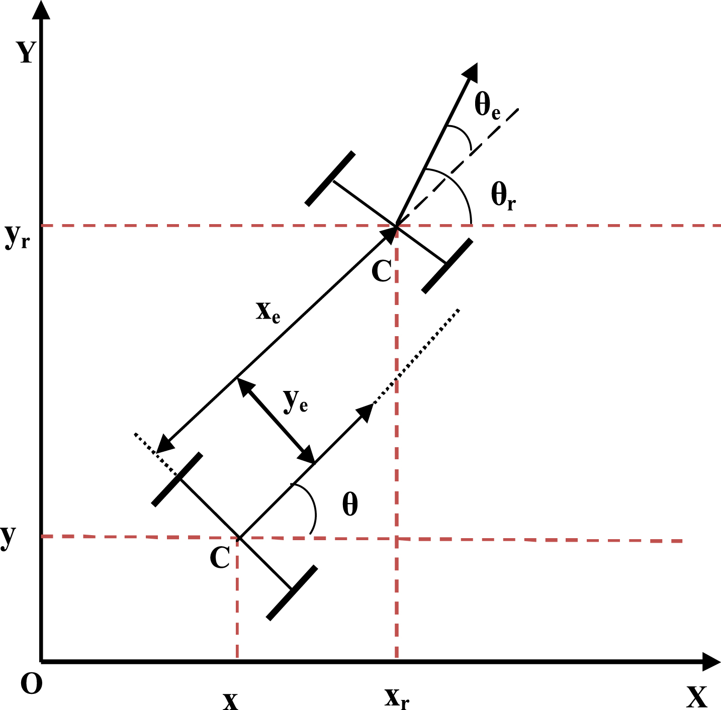
Posture error description.

According to coordinate transformation, the posture error equation of the mobile robot is described as:

$q_{e} = [\begin{matrix} x_{e} \\ y_{e} \\ θ_{e} \end{matrix}] = [\begin{matrix} \cos θ & \sin θ & 0 \\ - \sin θ & \cos θ & 0 \\ 0 & 0 & 1 \end{matrix}] [\begin{matrix} x_{r} - x \\ y_{r} - y \\ θ_{r} - θ \end{matrix}]$ (4)

When the matrix P can be written as: $P = [\begin{matrix} \cos θ & \sin θ & 0 \\ - \sin θ & \cos θ & 0 \\ 0 & 0 & 1 \end{matrix}]$ For the considered mobile robot, the trajectory tracking error is given by Equation (5). ${\begin{matrix} x_{e} = \cos θ (x_{r} - x) + \sin θ (y_{r} - y) \\ y_{e} = - \sin θ (x_{r} - x) + \cos θ (y_{r} - y) \\ θ_{e} = θ_{r} - θ \end{matrix}$ (5)

The equation, characterizing the slip-free rolling of a wheel on the ground, representing the nonholonomic constraints is presented in Equation (6). $\dot{x} s i n θ + \dot{y} c o s θ = 0$ (6)

Using the Equation (6) and some trigonometric relations, the derivative of the Equation (5) can be obtained as below: ${\dot{q}}_{e} = [\begin{matrix} {\dot{x}}_{e} \\ {\dot{y}}_{e} \\ {\dot{θ}}_{e} \end{matrix}] = [\begin{matrix} y_{e} ω_{c} - v_{c} + v_{r} cos θ_{e} \\ - x_{e} ω_{c} + v_{r} sin θ_{e} \\ ω_{r} - ω_{c} \end{matrix}]$ (7)

2.2 Dynamic model

Dynamic modeling in general is the study of the system motion in which forces are modeled and it can include energies and the associated speeds.

The general dynamic model can be described by Equation (8).

$\begin{matrix} M (q) \ddot{q} + V (q, \dot{q}) \dot{q} + F (\dot{q}) + G (q) + τ_{d} = B (q) τ \\ - A^{T} (q) λ \end{matrix}$ (8)

Where: M (q) is the symmetric positive definite inertia matrix, $V (q, \dot{q})$ is the centripetal and coriolis matrix, $F (\dot{q})$ is the surface friction matrix, G (q) is the gravitational vector, τ_d denoted bounded unknown disturbances including unstructured dynamics, B (q) is the input transformation matrix, τ is the input vector, A^T (q) is the matrix associated with the constraints, λ is the vector of the constraint forces.

The above system can be transformed into a more proper representation for control and simulation purposes. Equations (9–11) are defined to do this transformation: $S (q) = [\begin{matrix} \cos θ & 0 \\ \sin θ & 0 \\ 0 & 1 \end{matrix}]$ (9) $\dot{q} = S ϑ$ (10) $\ddot{q} = \dot{S} ϑ + S \dot{ϑ}$ (11)

The matrix S (q) has the following relation with A (q) matrix: $S^{T} (q) A^{T} (q) = 0$ (12)

Replacing Equations (10 and 11) in Equation (8), and multiply this last by S^T (q), therefore Equation (8) can rewrite itself as: $Mh (q) \dot{ϑ} + Vh (q, \dot{q}) ϑ + τ_{h} = Bh (q) τ$ (13)

With: $Mh (q) = S^{T} (q) M (q) S (q)$ (14) $τ_{h} = S^{T} (q) τ_{d}$ (15) $Bh (q) = S^{T} (q) B (q)$ (16) $Vh = S^{T} (q) M (q) \dot{S} (q) + S^{T} (q) V^{T} (q, \dot{q}) S$ (17)

G (q)= 0, because the motion is constrained to the ground.

$F (\dot{q})$ = 0, considered to be zero.

Equation (13) is the equation which is used for the control and simulation analysis of the robot. The dynamic modeling of the robot is presented in [22].

3 RBF neural network

RBF networks are adaptively used to approximate the uncertain nonlinear function. The algorithm of a radial basis function (RBF) networks is defined in [20] as: $\begin{matrix} h_{j} = g (z - c_{ij}^{2}) / b_{j}^{2}) \\ f = W^{t} h (z) + ɛ \end{matrix}$ (18)

Where z is the input state of the network, i is the input number of the network, j is the number of hidden layer nodes in the network, h = [h₁ h₂ … h_n] ^T is the output of Gaussian function. W is the neural network weights, and ɛ ≤ ɛ_N.

RBF network approximation f is used. The output of RBF network is: $\hat{f} (z) = {\hat{W}}^{T} h (z)$ (19)

The Fig. 2 represents an RBF network.

Fig. 2

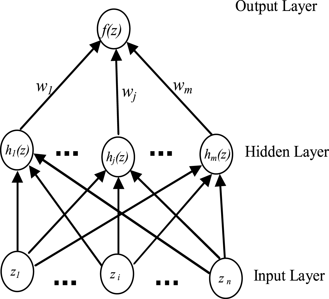
RBF Network.

The Gaussian function can be defined as:

$h (z) = exp (- \frac{r^{2}}{2 σ^{2}})$ (20)

4 Strategy of control

The control strategy in this work is based on two controllers, a kinematic controller and a dynamic controller whose objective is to put the robot following its reference trajectory in presence of disturbances. A neural controller is chosen to approximate the function f.

The Fig. 3 resumes this control strategy.

Fig. 3

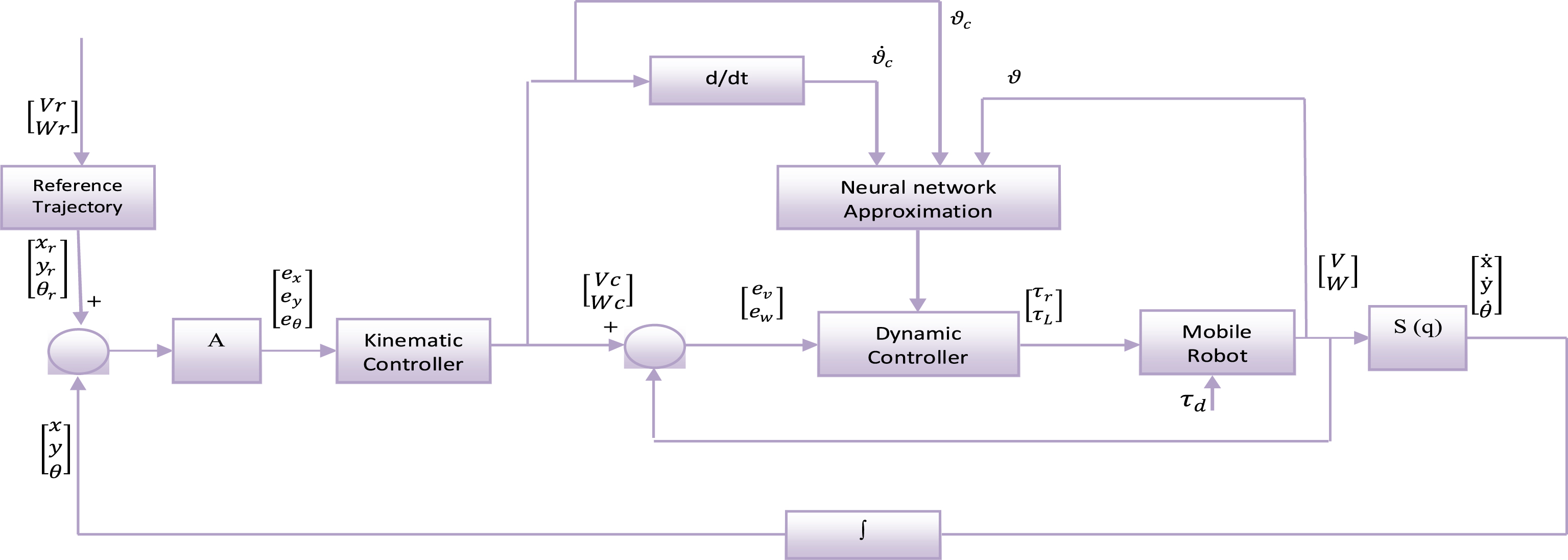
Control strategy diagram.

4.1 Kinematic controller

The kinematic controller is based on fast Terminal sliding mode control and permit to obtain the adequate velocities for an eventual stability in a finite time. The convergent characteristic of fast terminal sliding mode control is superior to that of the normal sliding mode control.

A kind of fast terminal sliding surface is proposed as follows: $s = \dot{x} + α x + β x^{q / p} = 0$ (21)

Where x ∈ R is the state and α > 0.

The reaching time of the sliding surface to zero is defined as: $t_{s} = \frac{p}{α (p - q)} ln \frac{α x (0)^{\frac{p - q}{p}} + β}{β}$ (22)

The global fast sliding surface is selected as: $s = {\dot{s}}_{0} + α s_{0} + β s_{0}^{q / p}$ (23)

Where α, β > 0 and q, p (q < p) are positives odd numbers.

4.1.1 Design of the angular velocity control law

According to Equation (7): ${\dot{θ}}_{e} = ω_{r} - ω_{c}$ (24)

The sliding surface is selected as: $s_{1} = θ_{e}$ (25)

Then Equation (24) can be rewritten as: ${\dot{θ}}_{e} = - θ_{e} - α_{1} θ_{e} - β_{1} θ_{e}^{q / p}$ (26)

The control law can be obtained as: $ω_{c} = ω_{r} + θ_{e} + α_{1} θ_{e} + β_{1} θ_{e}^{\frac{q}{p}}$ (27)

Theorem. consider Equation (24), there exist the control law (26) such that the system (24) is stable.

Proof. According to Equation (26), the Lyapunov function is described by: $V = \frac{1}{2} θ_{e}^{2}$ (28)

The derivate of the Lyapunov function is: $\begin{matrix} \dot{V} = θ_{e} {\dot{θ}}_{e} = (- θ_{e} - α_{1} θ_{e} - β_{1} θ_{e}^{\frac{q}{p}}) θ_{e} \\ = - θ_{e}^{2} - α_{1} θ_{e}^{2} - β_{1} θ_{e}^{\frac{q + p}{p}} \end{matrix}$ (29)

Such that p > 0 and q > 0 are odd integers, α₁ > 0 and β₁ > 0, then: $\dot{V} \leq 0$

4.1.2 Design of the linear velocity control law

Notice that when θ_e converges to 0, then ω_r = ω_c. Another two state control design are considered in this time: ${\dot{x}}_{e} = ω_{r} y_{e} - v_{c} + v_{r}$ (30) ${\dot{y}}_{e} = - ω_{r} x_{e}$ (31)

The switching function can be designed as follows: $s_{2} = x_{e} - y_{e}$ (32)

By designing sliding mode control law that s₂ → 0, the state x_e converges to y_e in order to achieve x_e → 0 and y_e → 0.

Using the terminal sliding mode control: ${\dot{s}}_{2} = - s_{2} - α_{2} s_{2} - β_{2} s_{2}^{q / p}$ (33)

Using Equations (30 and 31) and the derivative of Equation (32), the above result is obtained: $ω_{r} y_{e} - v_{c} + v_{r} + ω_{r} x_{e} = - s_{2} - α_{2} s_{2} - β_{2} s_{2}^{q / p}$ (34)

Then, the forward velocity control law can be obtained as: $v_{c} = v_{r} + ω_{r} x_{e} + ω_{r} y_{e} - s_{2} - α_{2} s_{2} - β_{2} s_{2}^{q / p}$ (35)

4.2 Dynamic controller

In this section two cases of dynamic controller are considered. The first case in absence of disturbances, then GFSM controller is introduced.

In the second case when the disturbances are introduced, the NN-GFSM is applied.

4.2.1 Control without disturbances

In the case of absence of disturbances, Equation (13) becomes: $Mh (q) \dot{ϑ} + Vh (q, \dot{q}) ϑ = Bh (q) τ$ (36)

The velocities error is defined as: $e_{ϑ} = ϑ_{c} - ϑ = [\begin{matrix} e_{v} \\ e_{ω} \end{matrix}] = [\begin{matrix} v_{c} - v \\ ω_{c} - ω \end{matrix}]$ (37)

The derivative of (37) is obtained as follow: ${\dot{e}}_{ϑ} = {\dot{ϑ}}_{c} - \dot{ϑ}$ (38)

According to Equations (36, 38) becomes: $\begin{matrix} Mh (q) ({\dot{ϑ}}_{c} - {\dot{e}}_{ϑ}) + Vh (q, \dot{q}) (ϑ_{c} - e_{ϑ}) = Bh (q) τ \\ Mh (q) {\dot{ϑ}}_{c} - Mh (q) {\dot{e}}_{ϑ} + Vh (q, \dot{q}) ϑ_{c} - Vh (q, \dot{q}) e_{ϑ} \\ = Bh (q) τ \end{matrix}$ (39)

The nonlinear function is defined as: $f (z) = Mh (q) {\dot{ϑ}}_{c} + Vh (q, \dot{q}) ϑ_{c}$ (40)

With $z = [ϑ_{c}^{T} {\dot{ϑ}}_{c}^{T} ϑ^{T}]^{T}$

Replacing (40) in (39): $- Mh (q) {\dot{e}}_{ϑ} - Vh (q, \dot{q}) e_{ϑ} + f (z) = Bh (q) τ$ (41)

Then, to obtain the control law, a sliding surface is choosing: $s_{3} = e_{ϑ}$ (42)

According to the Equations (23, 42, 43) is established. ${\dot{e}}_{ϑ} = - (α_{3} + 1) e_{ϑ} - β_{3} e_{ϑ}^{q_{3} / p_{3}}$ (43)

Replacing Equations (41 in 43): $\begin{matrix} Mh (q) ((α_{3} + 1) e_{ϑ} + β_{3} e_{ϑ}^{q_{3} / p_{3}}) - Vh (q, \dot{q}) e_{ϑ} + \\ f (z) = Bh (q) τ \end{matrix}$ (44)

The obtained control law is: $τ = {Bh}^{- 1} (C_{v} e_{ϑ} + f (z) + β_{3} Mh (q) e_{ϑ}^{q_{3} / p_{3}})$ (45)

Such that: $C_{v} = Mh (q) (α_{3} + 1) - Vh (q, \dot{q})$ (46)

4.2.2 Control in presence of disturbances

In this case, the neural network controller is introduced.

The Equation (41) is defined as: $- Mh (q) {\dot{e}}_{ϑ} - Vh (q, \dot{q}) e_{ϑ} + f (z) - τ_{d} = Bh (q) τ$ (47)

The control law designed in Equation (45) becomes: $τ = {Bh}^{- 1} (C_{v} e_{ϑ} + \hat{f} (z) + β_{3} Mh (q) e_{ϑ}^{q_{3} / p_{3}})$ (48)

Where $\hat{f} (z)$ is the output of RBF network and $\hat{f} (z)$ approximates f (z).

RBF network can be adopted to approximate f (z). The desired algorithm of RBF network is: $φ_{i} = g ({∥ z - c_{i} ∥}^{2}) / b_{i}^{2}) i = 1, 2, …… . . n$ (49) $ζ = W^{* T} φ (z)$ (50) $f (z) = W^{* T} φ (z) + ɛ$ (51)z is the input state of network, φ (z) = [φ₁ φ₂ … φ_n] ^T, ɛ is the approximation error and W* is the weight vector of desired RBF network.

Replacing Equations (47 in 48).

$\begin{matrix} Mh (q) {\dot{e}}_{ϑ} = - (Vh (q, \dot{q}) + C_{v}) e_{ϑ} + μ_{0} \\ - β_{3} Mh (q) e_{ϑ}^{q_{3} / p_{3}} \end{matrix}$ (52)

When $μ_{0} = \tilde{f} (z) - τ_{d}$ , and $\tilde{f} (z) = f (z) - \hat{f} (z)$

The output of the network is given as: $\hat{f} (z) = {\hat{W}}^{T} φ (z)$ (53)

Selecting $\hat{W} = W^{*} - \hat{W}$ , ∥W^* ∥ ≤ W_max

Therefore: $μ_{0} = \tilde{f} (z) - τ_{d} = {\hat{w}}^{T} φ (z) + ɛ - τ_{d}$ (54)

The control law designed in Equation (48) becomes: $τ = {Bh}^{- 1} (C_{v} e_{ϑ} + \hat{f} (z) + β_{3} Mh (q) e_{ϑ}^{\frac{q_{3}}{p_{3}}}) - ξ$ (55)

Where ξ is the robust element introduced to eliminate the network approximation error ɛ and the disturbances τ_d.

Replacing Equations (52 in 54): $\begin{matrix} Mh (q) {\dot{e}}_{ϑ} = - (Vh (q, \dot{q}) + C_{v}) e_{ϑ} - β_{3} Mh (q) e_{ϑ}^{q_{3} / p_{3}} \\ + {\hat{W}}^{T} φ (z) + ɛ - τ_{d} + ξ \end{matrix}$ (56)

Putting: $μ_{1} = {\hat{W}}^{T} φ (z) + ɛ - τ_{d} + ξ$ (57)

Replacing Equations (54 in 55): $\begin{matrix} Mh (q) {\dot{e}}_{ϑ} = - (Vh (q, \dot{q}) + C_{v}) e_{ϑ} - β_{3} Mh (q) e_{ϑ}^{q_{3} / p_{3}} \\ + μ_{1} \end{matrix}$ (58)

The robust element ξ is designed as: $ξ = - (ɛ_{N} + b_{d}) sign (e_{ϑ})$ (59)

Where: ∥ɛ ∥ ≤ ɛ_N, ∥τ_d ∥ ≤ b_d

The candidate function of Lyapunov is selected as: $ρ = \frac{1}{2} e_{ϑ}^{T} Mh (q) e_{ϑ} + \frac{1}{2} tr ({\hat{W}}^{T} F_{w}^{- 1} \hat{W})$ (60)

The derivative of the Lyapunov function is defined as: $\dot{ρ} = e_{ϑ}^{T} Mh (q) {\dot{e}}_{ϑ} + \frac{1}{2} e_{ϑ}^{T} \dot{Mh} (q) e_{ϑ} + tr ({\tilde{W}}^{T} F_{w}^{- 1} \tilde{W})$

From Equation (56): $\begin{matrix} \dot{ρ} = - e_{ϑ}^{T} Mh (q) (α + 1) e_{ϑ} - e_{ϑ}^{T} β Mh (q) e_{ϑ}^{q_{3} / p_{3}} + \\ tr {\tilde{W}}^{T} (F_{w}^{- 1} \tilde{W} + φ (z) e_{ϑ}^{T}) + e_{ϑ}^{T} (ɛ - τ_{d} + ξ) \end{matrix}$ (61)

Selecting $\tilde{W} = F_{w} φ (z) e_{ϑ}^{T}$

The adaptive rule of network is: $\hat{W} = F_{w} φ (z) e_{ϑ}^{T}$ (62)

Therefore: $\begin{matrix} \dot{ρ} = - e_{ϑ}^{T} Mh (q) (α + 1) e_{ϑ} - e_{ϑ}^{T} β Mh (q) e_{ϑ}^{q_{3} / p_{3}} + \\ e_{ϑ}^{T} (ɛ - τ_{d} + ξ) \end{matrix}$ (63)

Considering the term: $\begin{matrix} e_{ϑ}^{T} (ɛ - τ_{d} + ξ) = e_{ϑ}^{T} (ɛ - τ_{d}) + e_{ϑ}^{T} ξ \\ = e_{ϑ}^{T} (ɛ - τ_{d}) - ∥ e_{ϑ} ∥ (ɛ_{N} + b_{d}) \leq 0 \end{matrix}$

Such that matrix Mh is defined positive, β₃ and α₃ are positives, therefore: $\dot{ρ} \leq 0$

5 Results and simulations

In this section the simulations are subdivided in two parts. Firstly, the GFSM dynamic controller is proposed, in the second part the NN-GFSM is introduced in order to deal the distrubances. The simulation using matlab/simulink is applied on the mobile robot system.

Let us consider a circular trajectory with: v_r = 1m/s, ω_r = 1 rad/s.

The disturbances τ_d = [0.1 . sin(t) 0.1 . cos(t)].

The matrices values of the dynamic model are taken from [4].

The circular trajectory is considered with the following values:

α₁= 4, β₁= 1, p₁= 7, q₁= 5, α₂= 0.5, β₂= 2, p₂= 7, q₂= 5. α₃= 1, β₃= 2, p₃= 7, q₃= 5. ɛ_N = 0.2, b_d = 0.1.

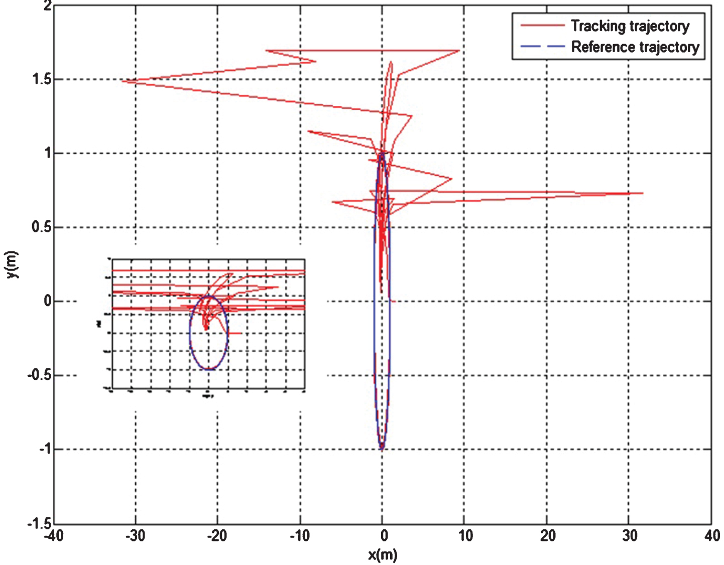
Figure 4 shows that the mobile robot diverges from the reference trajectory in the presence of disturbances. Therefore, the GFSM control stabilizes the system in finite time in the absence of disturbances, but cannot stabilize it in presence of disturbances.

Fig. 4

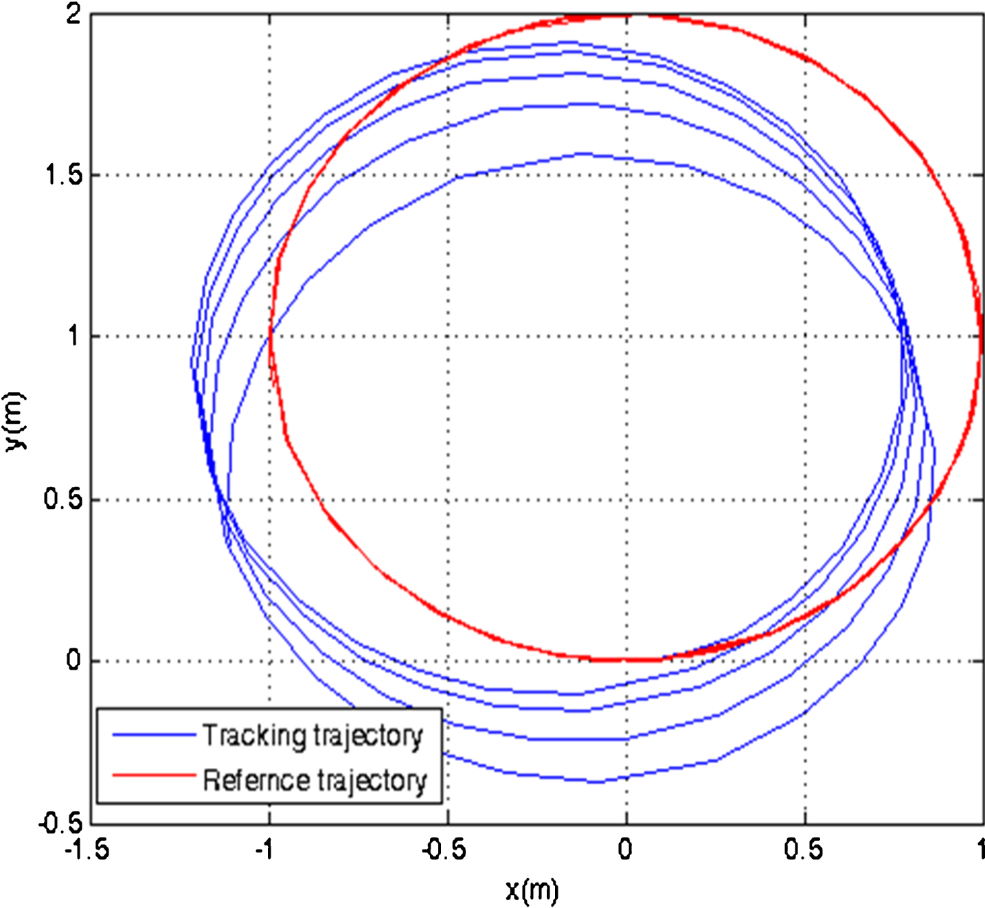
GFSM circular trajectory tracking.

Figures 5 and 6 show that actual linear and angular velocities of the proposed control could not keep up with the desired ones in presence of distrubances, therefore the tracking is degraded when the distrubances are appeared.

Fig. 5

GFSM linear velocities.

Fig. 6

GFSM angular velocities.

Figure 7 shows the control torques obtained in presence of distrubances.

Fig. 7

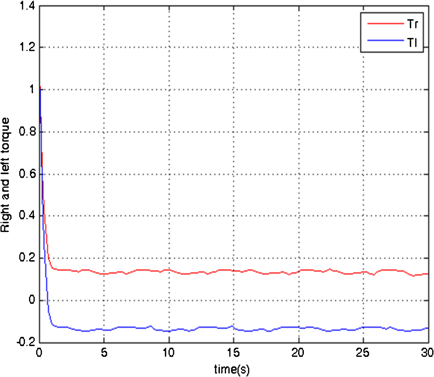
GFSM control inputs torques.

In the second part of simulation a NN-GFSM controller is introduced to deal the distrubances.

The circular trajectory is considered with the following values: α₁= 4, β₁= 1, p₁= 7, q₁= 5, α₂= 0.5, β₂= 2, p₂= 7, q₂= 5, α₃= 1, β₃= 2, p₃= 7, q₃= 5. ɛ_N= 0.2, b_d = 0.1.

The neural network is chosen with seven hidden, the initial weight matrix is selected as 0.1. b = 10.

Figure 8 shows the circular tracking trajectory with NN-GFSM control, the tracking trajectory diverges from the reference in first time, but it tracks the reference after a finite time. When the NN-FGSM tracking results compared with the precedent results, it is clear that the performance of the system has been improved with respect to the previous cases.

Fig. 8

NN-GFSM circular tracking trajectory.

Figure 9 shows that the tracking errors converge to zero in finite time.

Fig. 9

NN-GFSM tracking errors.

Figures 10 and 11 show the actual forward and angular velocities respectively of the NN-GFSM could keep up the desired ones in presence of disturbances. Figure 12 represents the control input torques. Figure 13 shows the estimated function of the non linear function.

Fig. 10

NN-GFSM linear velocities.

Fig. 11

NN-GFSM angular velocities.

Fig. 12

NN-GFSM control inputs torques.

Fig. 13

Non linear function and estimated function.

6 Conclusion

In this paper a NN-GFSM control is proposed to ensure the trajectory tracking of mobile robot, taking into account the dynamics of the robot.The proposed controller NN-GFSM reduces the errors and makes the system converges to the reference in a finite time. The NN controller stabilizes the velocities errors, deal the disturbances and approximate the nonlinear function.

Simulations results have demonstrated that the NN-GFSM controller is efficiency and gives the best performances in comparison with GFSM in presence of disturbances.

References

Antonelli ,

Chiaverni and

Fusco ,Afuzzy logic based approach for mobile robot path tracking, IEEE Trans Fuzzy Syst 15(2) (2007), 211–221.

Chwa , Sliding-mode tracking control of nonholonomic wheeled mobile robots in polar coordinates, IEEE Trans Contr Syst Technol 12(4) (2004), 637–644.

H.B.

Du ,

S.H.

Li and

C.J.

Qian , Finite-time attitude tracking control of spacecraft with application to attitude synchronization, IEEE Trans Autom Contr 56(11) (2011), 2711–2717.

Duc Do ,

Zhong-Ping and

Pan , A global output-feedback controller for simultaneous tracking and stabilization of unicycle-type mobile robots, IEEE Trans Automat Contr 30(3) (2004), 589–594.

Filipescu ,

Minzu ,

Dumitrascu ,

Filipescu and

Minca , Trajectory-tracking and discrete-time slidingmode control of wheeled mobile robots, IEEE International Conference on Information and Automation, 2011, pp. 27–32.

Fu ,

T.Y.

Chai ,

C.Y.

Su and

Jin , Motion/force tracking control of nonholonomic mechanical systems via combining cascaded design and backstepping, Automatica 49(12) (2013), 3682–3686.

Fukao ,

Nakagawa and

Adachi , Adaptive tracking control of a nonholonomic mobile robot, IEEE Transactions on Robotics and Automation 16(5) (2000), 609–615.

J.S.

Huang ,

C.Y.

Wen ,

Wang and

Z.P.

Jiang , Adaptive stabilization and tracking control of a nonholonomic mobile robot with input saturation and disturbance, Syst Contr Lett 62(3) (2013), 234–241.

C.L.

Hwang , A novel Takagi-Sugeno-based robust adaptive fuzzy sliding-mode controller, IEEE Transactions on Fuzzy Systems 12(5) (2004), 676–687.

10.

Huaguang ,

Jian ,

Yingchun and

Xiuhua , Sensor Fault Estimation of Switched Fuzzy Systems with Unknown Input, Accepted in IEEE Transactions On Fuzzy Systems, 2017.

11.

J.O.

Jang , Adaptive neuro-fuzzy network control for a mobile robot, Journal of Intelligent and Robotic Systems 62 (2011), 567–586.

12.

Khoo ,

Xie and

Man , Robust finite-time consensus tracking algorithm for multirobot systems, IEEE/ASME Transactions on Mechatronics 14(2) (2009), 219–228.

13.

Khoo ,

Ying ,

Man and

Yu , Finite-time stabilization of stochastic nonlinear systems in strict-feedback form, Automatica 49(5) (2013), 1403–1410.

14.

Kozlowski and

Majchrzak , A backstepping approach to control a nonholonomic mobile robot, In Proceedings of IEEE International Conference on Robotics and Automation, 4, 2002, pp. 3972–3977.

15.

S.H.

Li ,

S.H.

Ding and

Li , Global set stabilization of the spacecraft attitude using finite-time control technique, International Journal of Control 82(5) (2009), 822–836.

16.

A.D.

Luca and

Oriolo , Modeling and control of nonholonomic mechanical systems, In Angeles

and Kecskemethy

, (eds.), Kinematics and Dynamics of Multibody Systems, Springer, New York, 1995, pp. 277–342.

17.

Mohareri ,

Dhaouadi and

M.M.

Shirazi , Intelligent neural network based controllers for path tracking of wheeled mobile robots:Acomparative analysis, IEEE International Workshop on Robotic and Sensors Environments (2010), pp. 1–6.

18.

Nganga-Kouya and

F.A.

Okou , Adaptive backstepping control of a wheeled mobile robot, 17th Mediterranean Conference on Control and Automation, 2009, pp. 85–91.

19.

M.Y.

Ou ,

S.H.

Li and

C.L.

Wang , Finite-time tracking control for nonholonomic mobile robots based on visual servoing, Asian Journal of Control 16(3) (2014), 1–13.

20.

Park and

I.W.

Sandberg , Universal approximation using radial-basis-function networks, Neural Computation 3 (1991), 246–257.

21.

B.S.

Park ,

S.J.

Yoo , J.

Park and

Y.H.

Choi , Adaptive neural sliding mode control of nonholonomic wheeled mobile robots with model uncertainty, IEEE Trans Contr Syst Technol 17(1) (2009), 207–214.

22.

Fierro and

F. L.

Lewis , Control of a Nonholonomic Mobile Robot Using Neural Networks, in IEEE Transactions on Neural Networks, (9), 1998, pp. 589–600.

23.

Samson , Velocity and torque feedback control of a nonholonomic cart, in Lecture Notes in Control and Information Science, C. Canudas deWit, Ed. Berlin, Germany: Springer-Verlag, 1991, pp. 125–151.

24.

K.T.

Song ,

C.H.

Lee and

C.C.

Teng , Tracking control of unicycle-modeled mobile robots using a saturation feedback controller, IEEE Transactions on Control Systems Technology, 2001, pp. 305–318.

25.

Y.P.

Tian and

K.C.

Cao , Time-varying linear controllers for exponential tracking of non-holonomic systems in chained form, Int J Robust Nonlin Contr 17(7) (2007), 631–647.

26.

Y.P.

Tian and

S.H.

Li , Exponential stabilization of nonholonomic dynamic systems by smooth time-varying control, Automatica 38(7) (2002), 1139–1146.

27.

Y.Q.

Wu ,

Wang and

G.D.

Zong , Finite-time tracking controller design for nonholonomic systems with extended chained form, IEEE Trans Circ Syst 52(11) (2005), 798–802.

28.

J.M.

Yang and

J.H.

Kim , Sliding mode control for trajectory tracking of nonholonomic wheeled mobile robots, IEEE Transactions on Robotics and Automation 15(3) (1999), 578–587.

29.

Zhanshan ,

Lei ,

Huaguang and

Geyang , Faulttolerant controller design for a class of nonlinear MIMO discrete-time systems via online reinforcement learning algorithm, IEEE Transactions On Systems 46(5) (2015), 2168–2216.