
Abstract
Wireless Sensor Networks (WSNs) are set to play an important role in the Internet of Things (IoT). WSNs are deployed for many IoT applications like Smart-Street Lighting, Smart-Grid, etc. Time Synchronization Protocol (TSP) is an important protocol in WSNs and it is used for many of its operations. Most of the existing TSPs for WSNs are simulation-based works, which do not fully prove their effectiveness for WSNs. Further, the Line-of-Sight (LOS) conditions in which the WSN nodes are deployed can significantly affect the performance of these TSPs. However, most of the existing protocols neither talk about the LOS conditions in which these protocols were tested nor prove their effectiveness for different LOS conditions. To address these aspects, a synchronization protocol for cluster-based WSNs called a Simple Hierarchical Algorithm for Time Synchronization (H-SATS) has been proposed in this work and its performance is tested on a densely deployed large-sized WSN testbed in different LOS conditions. Further, H-SATS has been compared with the traditional regression-based method, which is the core synchronization scheme for different synchronization protocols in clustered WSNs. Experiments show that H-SATS outperforms the regression method in terms of synchronization accuracy to a maximum of 26.7% for a 30-node network.
Keywords
Introduction
Rapid technological advancements made over the past 30 years has made it possible to connect over the internet not just computers but also different appliances, devices, etc. This has led to the advent of the Internet of Things (IoT). Wireless Sensor Network (WSN) is set to play an important role in the IoT. WSNs are an integral part of many IoT applications like smart-street lighting systems [3], smart city [13], smart grids [27], etc. Also, WSNs have been used for various applications like agriculture [24], industrial monitoring [17], environmental monitoring [20], home automation [12], object tracking [8], personal health monitoring [2], etc. Some inherent advantages of WSN like low cost, low data bandwidth requirements, bidirectional communication capabilities, etc. [32] make it suitable for the IoT applications.
A WSN is a network of a number of devices called nodes, which are responsible for cooperatively sensing an event or phenomenon locally. Each node is typically equipped with relevant sensor(s), a microcontroller to provide the intelligence and a radio for communication. WSNs are characterized by low data rates, low power consumption, ad-hoc joining and leaving of nodes, self-configuring and self-healing capabilities during link failures, etc. Most of the nodes in the network are battery powered because they are often deployed in an environment where a continuous power source is not available.
Time Synchronization Protocol (TSP) is one of the most important protocols in a distributed network like WSN. TSPs provide a common reference of time either for the entire network or for some part(s) of the network. The common time reference provided by a TSP could be either (i) an absolute time like Coordinated Universal Time (UTC)/local time for a zone or (ii) relative/local time which is specific to the network or part of the network or (iii) just provide a basis to decide the chronology of some events in the WSN. The kind of time reference provided by a TSP depends on the requirements of the WSN application. TSP plays an important role in applications/functions like data gathering and fusion, time-based localization, TDMA based communication, power management protocols, etc. Time-Synchronization is all the more important for a WSN used in an IoT network because the sensor data recorded by a WSN is monitored and analyzed at remote locations. Thus, it is important to timestamp such sensor data according to a common clock valid across this IoT network. But generic TSPs like NTP [7] are not suitable for a WSN which has limitations like low bandwidth, low energy availability, etc. It is possible to achieve time synchronization among the WSN nodes if they are all equipped with devices like Global Positioning System (GPS) modules. But it is not possible to have a GPS module on every node as it increases the cost of each node tremendously. Further, GPS connectivity is very limited in indoor locations, in cloudy conditions, etc. [14]. We elaborate on the requirements and characteristics of a TSP in WSN in the next section.
There are several TSPs which have been proposed and even used in WSNs like RBS [14], TPSN [28], FTSP [25], SLTP [29], L-SYNC [21], etc. Many of them have demonstrated a synchronization accuracy of the order of microseconds while others have demonstrated an accuracy of lower orders. But there are very few protocols which have been demonstrated on a hardware testbed. We require a TSP which is simple and efficient (in terms of the computations involved), accurate, and which has been proved suitable for WSN on a hardware platform. Also, most of the works do not describe the environment in which the experiments have been performed. The environmental conditions, i.e., whether the communicating nodes are Line-of-Sight (LOS) or Non-Line-of-Sight (NLOS) significantly affects the performance of a TSP, especially in IoT applications which have NLOS environments (like Home Automation application). We, therefore, propose a Simple Hierarchical Algorithm for Time Synchronization (H-SATS) whose performance has been tested in this work on a large size testbed. Further, we show its performance compared to other relevant protocols in different environmental conditions like dense LOS and a mixture of LOS and NLOS network. The scope of this work is limited to WSNs in which the nodes are organized into clusters i.e. a cluster-based WSN. We will elaborate on the reasons for choosing cluster-based WSN in the next section.
The contributions of this paper are as follows: It presents H-SATS which is a simple and efficient TSP for a hierarchical clustered WSN. It achieves microsecond synchronization accuracy for varying network sizes. It shows the performance of H-SATS on a real WSN testbed. It also reports a performance analysis carried out for different LOS conditions which proves the degree of effectiveness of H-SATS in different environments.
Rest of the paper is organized as follows. Section 2 discusses the background of this work and previous works related to this paper. We describe H-SATS along with its mathematical basis in Section 3. The experimental setup and the methodology used to demonstrate our algorithm are described in Section 4.The results of the experiments performed on the hardware testbed have been presented and analyzed in Section 5. Finally, Section 6 offers conclusions.
Literature survey
Background
In a WSN, each node keeps its own local time using cheap crystal oscillators which do not have a very precise clock tick rate. However, we cannot use high-precision crystal oscillator on every node as it increases the cost of the network tremendously. Further climatic conditions like temperature, humidity, etc. and aging of the crystals affects the accuracy of the local time at these nodes [9]. Therefore it is very essential to synchronize these nodes to a level of accuracy required by the application. Some industrial, health and automotive applications require a micro-second accuracy time synchronizationprotocol [1].
Time synchronization in WSN is particularly challenging as the nodes are deployed in harsh environments like industrial plants [17], volcanoes [11], etc. They are deployed for unattended operation targeted to work with minimal or no maintenance, generally for a few months to a couple of years. Thus the synchronization protocol must be
As stated earlier, it is not possible for all the nodes in a WSN to be equipped with either a GPS device or high accuracy crystal oscillator. Thus each network typically consists of either one or few nodes called the anchor or master nodes which provide the time reference for synchronization of all other nodes in the network which are involved in the synchronization process. These anchor nodes are either equipped with a GPS device or they simply provide the reference for the local clock of the network. All other non-anchor nodes determine their local clocks with respect to these anchor nodes. These non-anchor nodes are called agent nodes [4, 5].
Time synchronization typically involves the exchange of packets between the anchor nodes and the agent nodes periodically. The period of such exchange depends on the level of synchronization accuracy required, the efficiency of the TSP, capabilities of the WSN nodes, etc. As stated above, it is desired that this period is as large as possible for the energy efficiency of the TSP and for prolonging the lifetime of the WSN nodes. However, various dynamic factors in a WSN like nondeterministic network access time, processor load on the WSN node, propagation time etc. cause time delays in the delivery of the packet to the receiver after it is generated at the sender. These delays like send time, access time, propagation time, reception time, receive time, etc. become a source of significant error in time synchronization. They have been elaborately discussed in [9, 25]. Of these, send time, receive time, access time and interrupt handling times are non-deterministic in nature while transmission and reception times and propagation delays are deterministic [25].
Having discussed the background of TSPs in WSN, we describe the related work in the next subsection.
Related work and problem addressed
As stated before, the focus of this work is a WSN with cluster-based topology. This kind of topology is extremely energy efficient, particularly in route formation, data fusion, etc. [21, 31] and these functionalities/applications are most common parts of a generic WSN. Thus we chose to focus our TSP for a clustered WSN. In a cluster-based topology, a few nodes are grouped together to form clusters. Each cluster has a cluster-head (CH) and other nodes are the cluster members (CMs).
TSPs for clustered WSN have been reported by L-SYNC [21], SLTP [29] and PC-Avg [23]. In PC-Avg, the CH collects information about the local time of its CMs, calculates its average and sends this average to the CMs. PC-Avg shows very poor synchronization accuracy and does not account for the previously mentioned non-deterministic and deterministic delays during packet transmission and reception. Also, it requires frequent synchronizations which undesirably increases the packet traffic in the network and thus decreases the lifetime of the nodes [29].
SLTP [29] and L-SYNC [21] synchronize the CMs to their respective CH. They use the regression-based scheme to improve the synchronization accuracy. SLTP and L-SYNC differ from each other in the way form the clusters. Both SLTP and L-SYNC have poor synchronization accuracy of the order of milliseconds, which is not sufficient for many applications. Also, they do not account for non-deterministic and deterministic delays in the packet transmission.
Recent works like CCTS [15] and CMTS [33] use consensus-based schemes to achieve synchronization. They perform an intra-cluster synchronization first which is followed by an inter-cluster synchronization to converge the virtual clocks on the nodes to a consensus clock. However, CCTS and CMTS use a large number of iterations to achieve convergence. Thus, they are not practically suitable for energy-constrained WSN nodes and thus we have not compared our protocol with CCTS and CMTS. Also, CCTS does not consider the non-deterministic delay in packet transmissions. It writes-off these delays by saying that MAC-layer timestamping will take care of these delays. But that is not true in reality [25].
Importantly, the performance of CMTS, CCTS, SLTP, L-SYNC, and PC-Avg have only been demonstrated on simulators. Their performance on a real WSN testbed and their suitability for WSNs is thus questionable. Simulator-based works cannot give a complete picture of the performance of a TSP as they make many assumptions at a high level of abstraction, they do not consider packet loss and its effect on synchronization accuracy [6]. Another aspect that the works on TSPs lack are that they do not do a performance analysis under different LOS conditions. The performance of a TSP is affected by the fact whether the communicating WSN nodes are in LOS condition or in NLOS condition. Thus, as the conditions vary, the results may vary. We need to know the degree of efficiency of a TSP in a given condition. This would also help us choose an appropriate TSP for a given scenario. We, therefore, address the above issues in our TSP called H-SATS that is presented in this paper. We discuss the methodology of H-SATS in the next section.
A typical network considered.
Clock model and mathematical basis
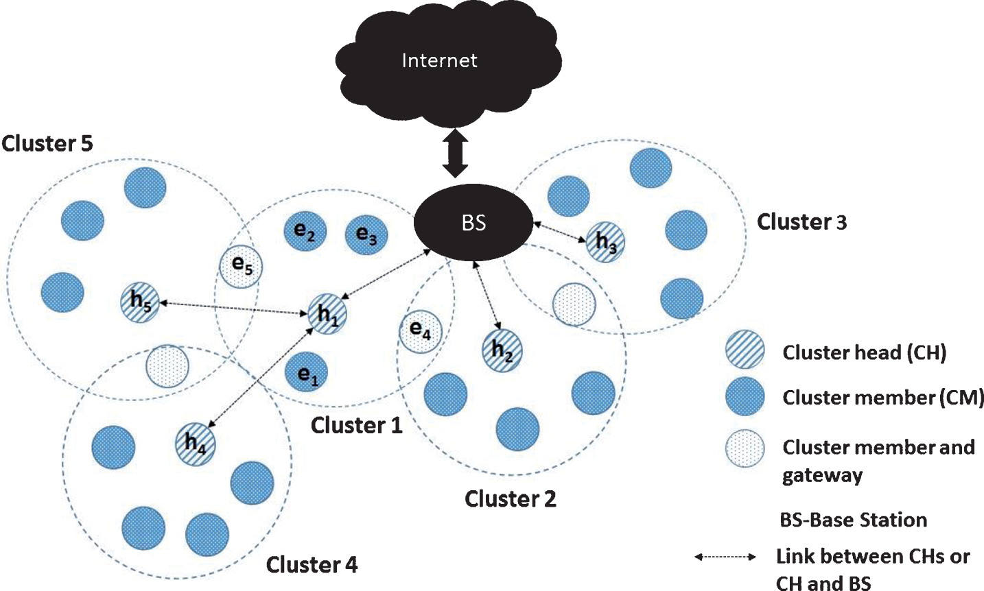
A typical network having a cluster based topology considered in H-SATS is shown in Fig. 1. A Base-Station (BS) is connected to the internet. All the cluster heads are connected to the BS either directly or in a hierarchical manner. A cluster consists of a cluster head and cluster members. Each cluster member communicates only to its CH. The CH nodes are chosen a priori on the basis of their hardware capabilities like superior computation capacity compared to a CM, availability of continuous power supply or greater battery energy availability, etc. We consider a network where nodes are stationary and assume that the nodes are connected via symmetric links for the sake of simplicity. A CM which can hear from more than one CH is called a gateway node. The network is divided into clusters using the cluster formation technique discussed in SLTP [29] or L-SYNC [21]. We can incorporate the feature by which all the nodes in the cluster become CH in turns so that no single node is burdened with CH role which could lead to draining of energy resources on that node.
We consider a WSN network consisting of n nodes defined by the set
We also define a function g CH (x, y), which tells whether a CH node y is a child of the BS or CH node x or not, i.e.
The clock model considered for this work is the skew-offset model [9, 18]. This model relates the local time of a node with the global time using the following equation.
H-SATS is a simple synchronization scheme which was presented in a preliminary form in [10]. In [10], all the CMs are synchronized to its CH only. The present work H-SATS extends [10] by achieving network-wide synchronization which is very helpful for a hierarchical WSN used in an IoT network. Further, this work also does a performance analysis of H-SATS for different LOS conditions, i.e., in a complete LOS condition where all the nodes in a cluster are LOS and a mixed-LOS condition where some CMs are LOS with their CH while other CMs are NLOS with their CH. A detailed explanation of the cluster-tree formation, cluster-formation phase, and the mathematical basis of H-SATS is also presented in this work. The CH tree formation phase and the cluster formation phase are described in the following subsection.
We refer to Fig. 1 to explain different phases of H-SATS. The BS initiates the CH tree formation phase by broadcasting Hello_packet. The BS is at level-0 and this level-information is also present in this Hello_packet of the BS. The CHs h1, h2, and h3 which are able to hear these packets assign themselves a level-1. These CHs, in turn, broadcast Hello_packet with its level information and also its id denoted as CH_ID. The CHs which hear these packets assign themselves as level-2 and also note the CH_ID of their parent CH. In the example that we are referring to in Fig. 1, h4 and h5 hear the Hello_packet sent by h1 and they become the children of h1. If a CH hears the Hello_packet of more than one parent CH, it chooses the CH whose packet is received with greater signal strength as its parent CH. In this way, CH tree is formed. Note that this CH tree formation is performed only once as the CHs are fixed and are stationary.
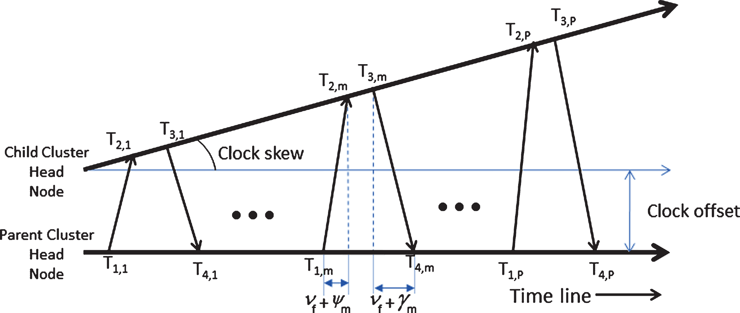
Two-way message exchange between parent CH head node and child CH node along the time axis.
The cluster tree formation phase is followed by the cluster formation phase. The CHs begin this phase by broadcasting the CM_joining packet. This packet also contains the CH_ID of the broadcasting CH. All the nodes (which are not CHs), which hear this CM_joining packet from a CH, join the cluster of that particular CH. In this case, the nodes e1, e2, e3, e4 and e5 hear the CM_joining packet of h1 and join the Cluster 1. A node which hears the CM_joining packets of multiple CHs joins the cluster of more than one CH. For instance, the node e4 hears the CM_joining packets of h1 and h2 and thus joins both Cluster 1 and Cluster 2. Such a node becomes a cluster gateway node as it is a part of more than one cluster. Since this gateway node has more than one CH, it records the CH_IDs of all its CHs. It sends this list of its CHs to all its CHs. So e4 sends the list of its CHs to h1 and h2 which will help h1 and h2 to communicate with each other through e4. After the cluster formation phase is complete, when a new node joins the network, it can search for a CH by broadcasting a CH_initial packet. Any CH which hears this packet and is ready to join this newly joining node into its cluster, responds to this packet. If the new node receives a response from more than one CH, it joins more than one cluster and it becomes a gateway node. This phase is followed by the synchronization phase.
The level-1 CHs are first synchronized to the BS. In Fig. 1, the BS synchronizes h1 (i.e.CH of cluster 1), h2 and h3. These CHs, in turn, synchronize their children CHs i.e. in this case h1 synchronizes h4 and h5. Once the CHs are synchronized, the CHs synchronize the CMs within their clusters. For instance, h1 synchronizes its own CMs i.e. e1, e2, e3, e4 and e5. The method by which a CH is synchronized with its parent CH is the same as the method by which a CM is synchronized with its CH. We first describe the procedure for synchronizing a CH with its parent. The parent could be a CH or the BS itself. In H-SATS each child CH is synchronized to its parent CH. Thus the clock model in Equation (3) can be written as
Synchronization in H-SATS is performed using a two-way message exchange between the parent CH and the child CH as represented in Fig. 2. The packets are time stamped by each node as per its local clock on a packet transmission and reception. The first packet was sent from the parent CH at T1,1 as per its local clock. This packet is received by the child CH at T2,1 as per its local clock. The child CH acknowledges this packet by sending another packet to the parent CH at T3,1 as per child CH’s local clock. The parent CH receives this acknowledgment packet at T4,1 as per its local clock. The packet exchanged between a child CH and its parent CH will contain the time stamps of transmission and reception, i.e., T1,1, T2,1, T3,1, and T4,1. MAC-layer timestamping as used in [25, 28] can be employed here to reduce the send time, access time and reception time delays in the transmission. Thus, when the acknowledgment packet is received at the parent CH, it gets all the four local time stamps of one complete two-way exchange. A total of P such two-way exchanges are performed between a parent CH and one child CH. Using Equation (4) we can relate the time stamps of an mth two-way exchange (where 1 ≤ m ≤ P) as follows
We observe from Equation (7) that as α
ih
, ν
f
and ψ
m
are always positive, T2,m lies above the line α
ih
T1,m + β
ih
. Similarly from Equation (8) we see that since α
ih
, ν
f
and γ
m
are always positive, T3,m lies below the line α
ih
T4,m + β
ih
. We know that α
ih
is the rate of child CH’s clock with respect to parent CH’s clock. So if we plot the timestamps of child CH (on the y-axis) with respect to parent CH’s timestamps, α
ih
is the slope and β
ih
is the y-intercept. So very good estimate of the α
ih
and β
ih
can be obtained by fitting a line for these points (T2,m, T1,m) and (T3,m, T4,m) where 1 ≤ m ≤ P. An approximate yet a good estimate for this fit-line can be obtained by taking two points M1 and M2 such that
From Equations (9 and 10), we can note that M1 refers to the two-way exchange with the least deterministic and non-deterministic delays while M2 refers to the next least. Thus when a line is drawn through M1 and M2, the slope of this line gives α
ih
and the intercept of it gives β
ih
. Thus we get
The above mentioned simple method to estimate the relative skew and offset has an accuracy comparable to the much complicated and computationally intensive maximum-likelihood estimate [26]. Note that [26] just gives the basis for this simple synchronization scheme and it is a simulation-based work. The current work improvises on this scheme by applying it for clustered WSN and demonstrates its efficacy on a testbed. Further, we have also employed the cluster tree formation, cluster formation phases and a schedule for message exchanges to achieve a network-wide synchronization. Once a CH is synchronized, it initiates the synchronization with its CMs. The CMs of a cluster are synchronized to their CH in the same method as a child CH is synchronized to the parent CH. Each CM performs Q two-way exchanges with its CH and then the relative offset and relative skew of a CM with respect to the CH is calculated.
Thus, after the synchronization phase, the CMs are synchronized to their CH and the CHs are synchronized to the BS. Thus, any sensor data that is recorded at a CM can be easily timestamped according to the internet time by the BS which is synchronized to the internet clock and also to a CM in the WSN. The algorithm of the synchronization phase of H-SATS is presented in Algorithm 1. The important notations used in this paper are summarized in Table 1.
Notation summary
Computational Complexity of H-SATS and regression-based method for synchronization between two nodes
In this subsection, H-SATS is compared with a regression-based synchronization scheme. The regression-based method has been used both in SLTP [29] and L-SYNC [21]. Both L-SYNC and SLTP have been shown to be scalable time synchronization algorithms for clustered WSN. As stated before, SLTP and L-SYNC differ from each other in the cluster formation method while both use linear regression in the synchronization phase. Linear regression-based synchronization method has very high computational complexity and thus is more expensive than H-SATS. The number of multiplications, as well as additions to be performed for time synchronization in the linear regression method, are much higher as compared to those in H-SATS. The computational complexities for synchronization between two nodes (for instance CH and its CM) are compared in Table 2. In this table, Q represents the two-way exchanges performed between the two nodes which are trying to get synchronized with each other (like a CM with its CH). H-SATS requires one subtraction (which can be seen as an addition) to calculate a two-way exchange’s duration which is computed by (T4,m - T1,m). Thus Q two-way exchanges require Q addition (or subtraction) operations. Further, 2 (Q - 2) subtractions are required for comparison operations to determine the two-way exchange with minimum delays. Further, 4 additions are required in Equations (9 and 10). It requires a total of 7 multiplications, 4 of which are required in Equations (9 and 10) and the rest of the 3 multiplications are required in Equation (12). The size of the timestamp variable in the microcontroller of a WSN node needs to be increased to 32-bits to maintain a clock of microsecond resolution and also to measure a considerable time duration before the clock overflows. When computationally intensive 32-bit multiplications are involved, a reduction in the number of multiplications to an order of 1 gives H-SATS a significant computational edge over regression-based method. WSN processors like MSP430 of TelosB WSN nodes may find it difficult to support the intense computations involved in the regression-based method. Powerful WSN nodes like NXP’s JN5179 [16] or Lotus [19], can execute such intensive computations as they are equipped with 32-bit processors. However, they do so at the cost of consuming higher processor time and power which is generally not desirable for energy constrained WSN nodes. Also, the use of such expensive powerful nodes inhibits their large-scale deployment in WSNs. Thus, H-SATS, which is less computationally intensive, is a suitable TSP for energy-constrained WSN nodes.
Experimental setup and methodology used
We have compared H-SATS with the traditional regression-based scheme on TelosB nodes [30] which are based on MSP-430, a 16-bit microcontroller. The network was organized to form clusters of 4 CMs and one CH, i.e., 5 nodes per cluster. These nodes were deployed in two different environments: Line of Sight(LOS)- where all the CMs and CH could communicate without any obstacle Mixed LOS-Mixture of LOS and NLOS where two of the CMs in a cluster were LOS and other two CMs were NLOS with their CH. We will refer to this environment as mixed-LOS environment for brevity in the future
We describe the experimental setup for the above two environments in the following sub-sections.
LOS environment
The WSN nodes were deployed in an open field as shown in Fig. 3. Each cluster was deployed in an area of 5 sq. meters. The inter-cluster distance was less than 1 meter, i.e., it is a very dense deployment. The experiment was initially performed with just one cluster turned on. Other clusters were turned on one-by-one gradually so as to generate the traffic which will help us analyze the performance of these algorithms in dense traffic conditions. A total of 30 WSN nodes, i.e., 6 clusters were used in this experiment. The CHs were first synchronized to the BS. Then the synchronization packets were exchanged between a CH and its CMs. The CH unicast the synchronization packets to each CM one-by-one and the CM replied to them via a unicast communication. However, the traffic caused by the packet exchange in one cluster did cause packet drops in other clusters. A snapshot of a part of the network deployed can be seen in Fig. 3. The WSN nodes are encircled in red.
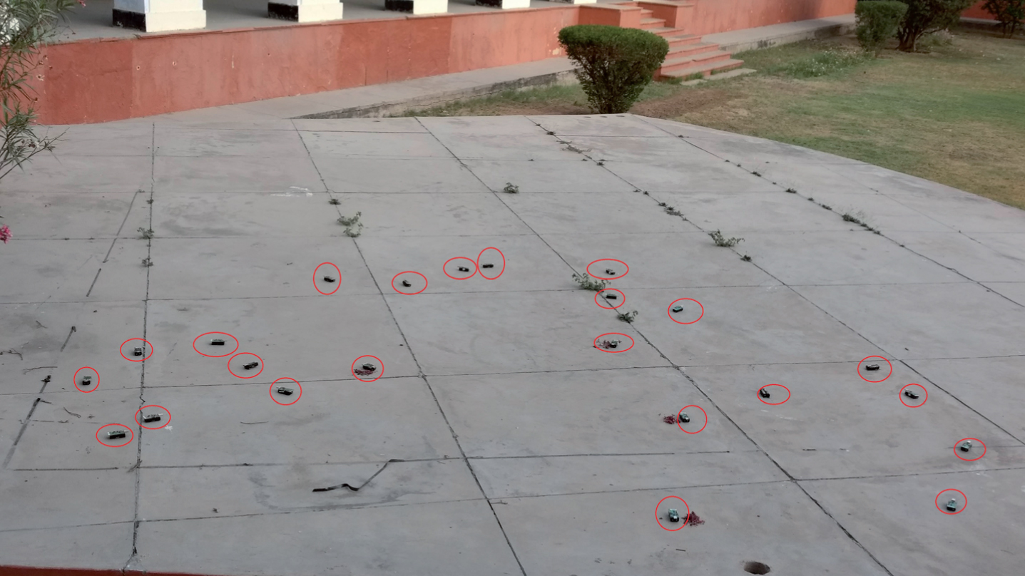
Picture showing part of the network deployed with WSN.
In this deployment, some of the nodes were placed inside a lab and the rest of the nodes were deployed in the gallery outside the lab (as shown in Fig. 4). The BS was inside the lab. The nodes in the gallery were separated from the nodes inside the lab by thick concrete walls. The CH of a cluster could communicate LOS with two of its CMs and other two CMs were in an NLOS position. These CMs in NLOS position with respect to their CH were separated by a thick concrete wall to provide a formidable obstacle for packet transmission. The experiment was performed with only one cluster turned on initially. The other clusters were turned on one-by-one to generate the traffic.
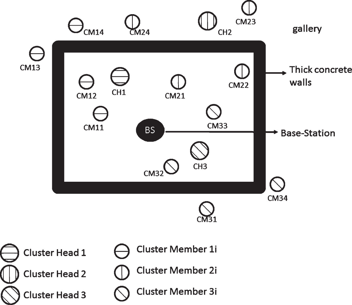
An indicative diagram depicting part of the deployment for mixed LOS (a mixture of LOS and NLOS) environment.
The methodology described in this subsection used to perform H-SATS and to compare it with the regression-based method is common to both environments mentioned previously. In H-SATS, as stated before, each CM is synchronized with its CH. In the current implementation, we employ a training phase to perform the synchronization and a testing phase to evaluate the performance of the TSP. The synchronization phase (i.e training phase) of H-SATS algorithm has been summarized in Algorithm 1. It is to be noted that the testing phase is not a part of the H-SATS algorithm as such. The training and testing phases are described below in detail.
Training phase
In this phase, each CH initiates two-way packet exchanges (described in section 3.1) with its parent CH (or the BS if the CH is level-1 CH). It performs P two-way exchanges with the parent CH (or BS) and it identifies the two-way exchanges with minimal and next minimal delays as shown in Equations (9 and 10). The relative offset and relative skew of the child CH with respect to the parent is calculated using Equations (11 and 12). This procedure is then repeated by all the CHs with all its CMs to synchronize the CMs to their respective CH. The only difference is each CH performs Q two-way exchanges with each of its CM one-by-one. In the current evaluations, P and Q values have been taken to be 17 the reason for which will be explained in the next section. Also, the timestamps of the two-way exchanges of all CHs with their CMs are forwarded to a PC which has the base-station (as shown in Fig. 5) connected to it. The calculations for H-SATS and regression method (i.e., to calculate the relative skew and offsets) are done on a PC in the current implementation. Figure 5 shows the base-station node connected to the PC on the left. The right side portion of the figure shows the zoomed portion of a part of the PC’s screen in which four timestamps collected for a single two-way exchange are encircled in red.
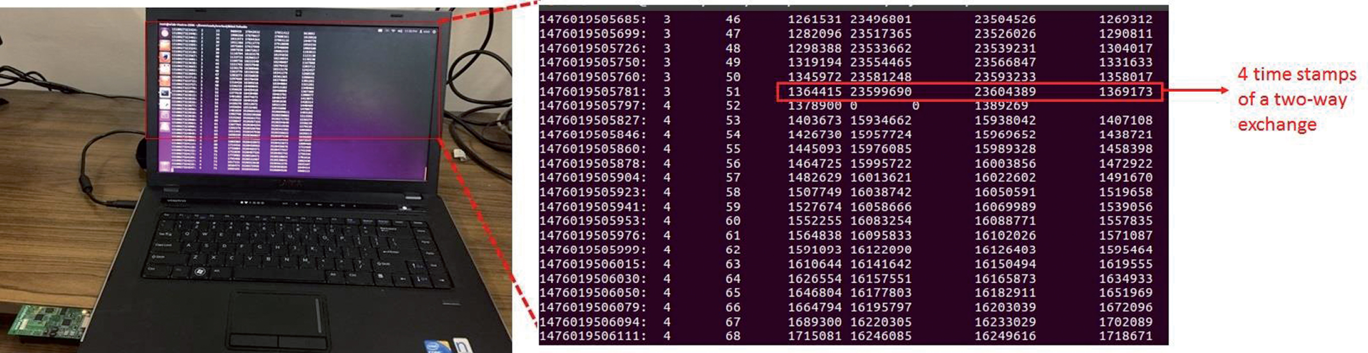
Base-station collecting the timestamps of the cluster and forwarding it to a PC. The right portion of the figure shows a zoomed out portion.
After the synchronization of all nodes is complete, we need to test the synchronization accuracy obtained by both the synchronization schemes. For this, we need to generate a common event which is observed by both the CH and the CMs in a cluster. The CH and CMs will record the occurrence of the event as per their local clock. Each CM will send its timestamp for that event to the CH. Using the Equation (4), the CH will estimate the local time of occurrence of the event as per each CM’s local clock by using its own local clock and the relative skew and offset estimated in the training phase. This estimated local time at each CM for the event occurrence is compared with the actual local time at each CM for event occurrence (which was sent by each CM to the CH individually). The difference in these estimated and actual times gives the synchronization error for each CM. This is repeated S times in each cluster, i.e., a common event is generated S times and the average synchronization error is calculated. The common event is generated by broadcasting packets (called testing packets) sent by an independent node which is not part of any cluster of this WSN. We refer to this node as the third-party node. This third-party node broadcasts the testing packets at a transmission power level sufficient for it to communicate to all the nodes in the WSN. In fact, having a dense deployment of the clusters makes the area of the network small enough for this third-party node to communicate to all the nodes. The propagation time of the testing packet from the third-party node to each node in the network is almost the same. This method of generating a common-event ensures that the event is seen almost at the same time by all the nodes in a cluster. Also, this method ensures that errors like send-time, access time, etc. do not affect the accuracy of the testing phase.
Results and Analysis
The nodes were deployed in two different environments as described in the previous section and synchronization error was calculated for H-SATS and the regression-based method. Each CH performed 17 two-way exchanges with each of its parent CH (or BS) and with each of its CM in training-phase, i.e., P= 17 and Q= 17. We have chosen this number of iterations by analyzing our experimental results. Figure 6(a) and (b) show experimentally obtained variation of synchronization error for different sized networks as a function of the number of two-way exchanges in LOS and mixed-LOS environments respectively. From these figures, we can see that as the number of two-way exchanges increase, the synchronization error shows very little variation. The third-party node was used to generate 15 common-event broadcast packets in testing-phase, i.e., S= 15. The synchronization error in microseconds for LOS environment deployment for networks of varying size is shown in Fig. 7a. The percentage increase in synchronization accuracy of H-SATS compared to the regression-based method for varying network size is shown in Fig. 7b. Note that we have referred to the regression-based method as regression method in Fig. 7a and 8a for brevity. For a 5-node network, i.e., when there was only one cluster in the network, the regression method gave a synchronization accuracy almost equal to H-SATS. But as the network size increases, H-SATS performed better than the regression method and there is a significant difference in synchronization error for a large network. In a 30-node network, H-SATS had a synchronization error of 158.3μs compared to the regression method’s 216μs. Thus H-SATS showed 26.7% better accuracy than the regression method as seen in Fig. 7b. This difference in performance can be understood from the fact that as the network size increases, there will be significant traffic in the network. This, in turn, increases packet drops, access times, receive time, transmission and reception times, thereby increasing deterministic and non-deterministic delays in packet transmission, particularly during the training phase. Performance of the regression method is affected by all the packets in the training phase and thus its accuracy decreases. On the other hand, H-SATS is affected by just two points M1 and M2, i.e., packets which have minimal deterministic and non-deterministicdelays.
The synchronization error in microseconds for the deployment in a mixed-LOS environment for various network sizes is shown in Fig. 8a. The percentage increase in synchronization accuracy of H-SATS compared to the regression method for varying network size is shown in Fig. 8b. In this network also, the regression method had almost the same accuracy as H-SATS for the 5-node network, i.e., when there is only one cluster in the network. There is a sharp increase in synchronization error for the regression method as the network size increases. For a 30-node network, the synchronization error for the regression method is 711.2μs compared to H-SAT’s 548.63μs, i.e., H-SATS has 22.83% better accuracy as seen in Fig. 8(b). As stated before, as traffic increases the non-deterministic and deterministic delays increase which affects the regression method more than H-SATS. Also, in the mixed-LOS environment where some nodes in the cluster are NLOS, we have observed greater packet drops in this deployment which increases the synchronization error. Also, we can see that the difference in synchronization error for a 30-node network between the two synchronization schemes is 57.7μs in a LOS environment. But this difference increases to 162.41μs in a mixed-LOS environment. Thus we see that as more and more nodes become NLOS, the advantage of H-SATS over the regression method in terms of synchronization accuracy increases.
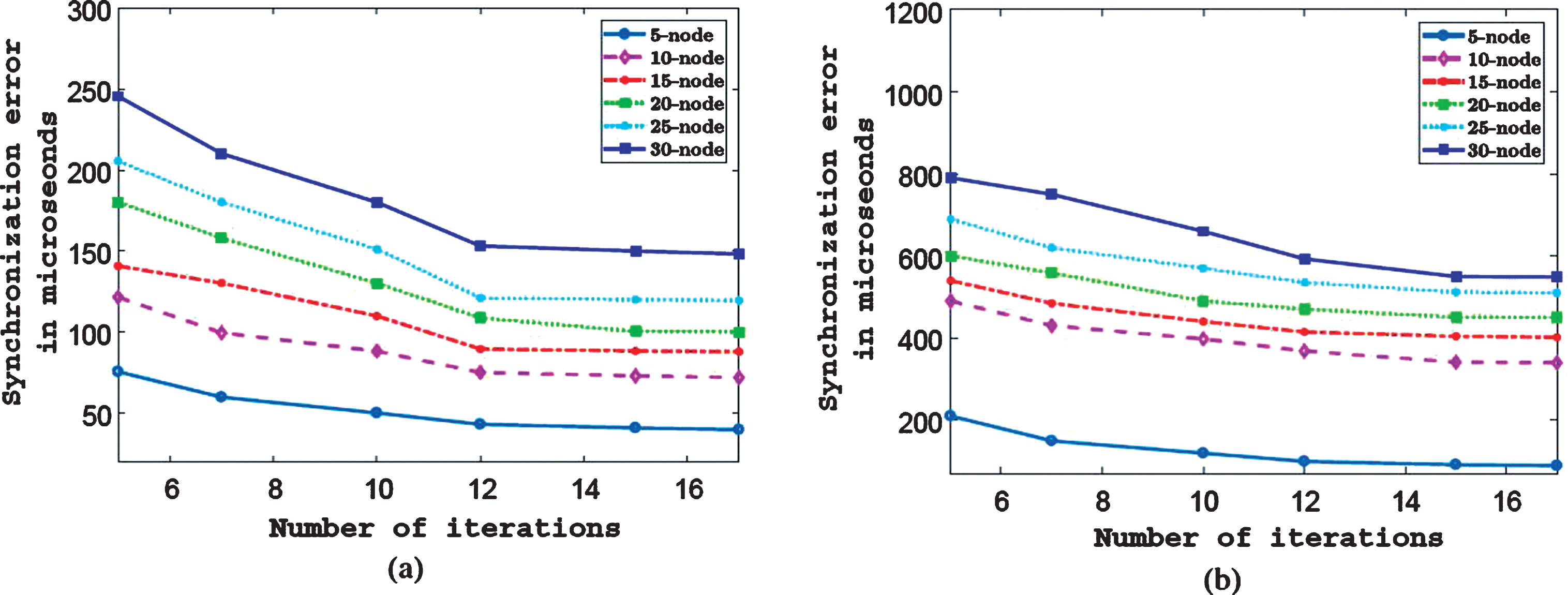
Variation of synchronization error with the number of two-way exchanges for varying network sizes (a) for LOS environment (b) for mixed-LOS environment.
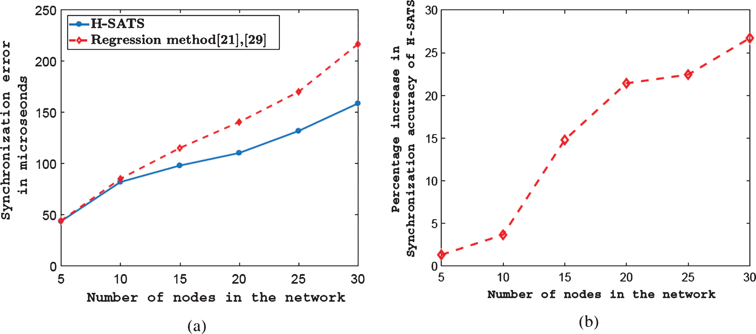
(a) Synchronization error for varying network sizes in LOS environment (b) Percentage increase in synchronization accuracy of H-SATS compared to regression method for varying network sizes in LOS environment.
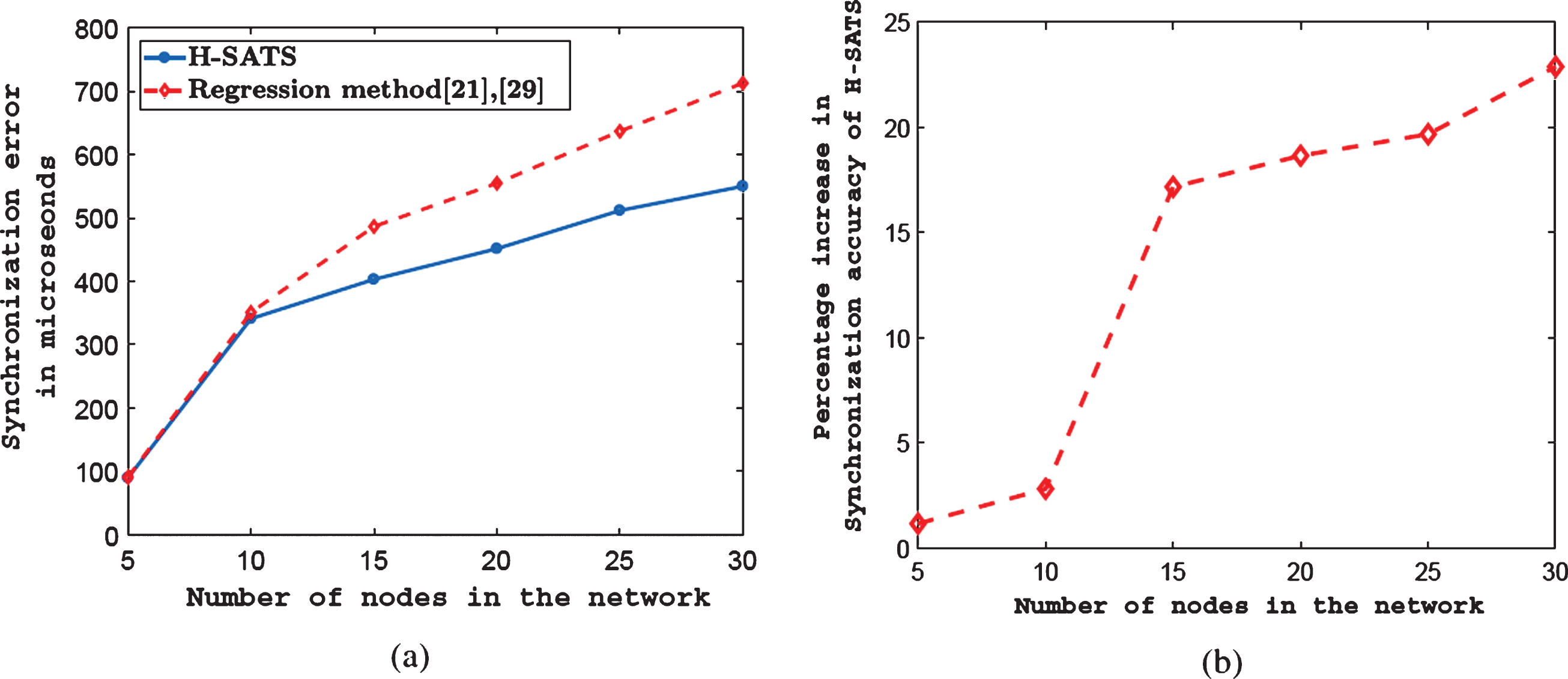
(a) Synchronization error for varying network sizes in the mixed-LOS environment (b) Percentage increase in synchronization accuracy of H-SATS compared to regression method for varying network sizes in the mixed-LOS environment.
We have described and implemented a simple yet accurate synchronization protocol called H-SATS for cluster-based stationary WSNs. H-SATS has also been compared to the regression method used in other TSPs for clustered WSNs. These tests were performed on a real WSN testbed which thus gives a credible proof of performance of H-SATS. H-SATS is computationally more efficient than the regression-based method which is very important for battery constrained WSN. Also, H-SATS has been analyzed in different LOS conditions, i.e., for completely LOS and for a mixture of LOS and NLOS conditions. This shows the stability in the performance of H-SATS in different environments. The difference in synchronization accuracy of H-SATS compared to the regression-based method increases with the network size. Also, in mixed-LOS environments, increase in the synchronization accuracy of H-SATS over the regression method is much higher than in LOS environments. Thus it is very important to choose a simple TSP like H-SATS in WSNs which has some nodes in NLOS condition. Further, we see that H-SATS is especially suited for large sized clustered WSN.