Construction and complexity analysis of new cubic chaotic maps based on spectral entropy algorithm

Abstract

This paper proposes two kind of new cubic chaotic maps based on Li-Yorke’s chaos criterion theorem, and gives the corresponding chaos discriminant conditions. The dynamical behaviors of systems are numerically simulated by nonlinear techniques including bifurcation diagrams and Laypunov exponents, and the simulation results show the cubic chaotic maps display chaotic characteristics as the provided theorems expect. Using spectral entropy algorithm, this paper analyses the complexity of chaotic sequences generated by cubic chaotic maps after quantitative process, and further compares the complexity of the chaotic pseudorandom sequences based on different quantitative methods. The results show different quantitative methods has a significant effect on the complexity of chaotic sequences; the pseudorandom sequences generated by the systems and quantitative method provided in this paper turns to have a better complexity. The above conclusions provide a theoretical basis for generating pseudorandom sequences with better quality.

Keywords

Cubic chaotic maps lyapunov exponent spectral entropy complexity

1 Introduction

Chaos is one special behavior of nonlinear dynamic systems, and has many applications in various fields nowadays. For chaos theory researchers, construction of new chaotic systems has been one of important subjects about chaos. In 1975, Li and Yorke proposed a criterion for existence of chaos in one-dimensional discrete systems. However, it is difficult to determine whether a cubic polynomial map is chaotic in terms of this criterion. So far, only a little related work is reported.

This paper firstly constructs two cubic polynomial maps with special form, and then uses the Li-Yorke’s chaos criterion theorem to find their chaos discriminant conditions. Secondly, the dynamical behaviors of systems are numerically simulated by nonlinear techniques including bifurcation diagrams and Laypunov exponents. Furthermore, the spectral entropy (SE) algorithm is applied to analyze the complexity of pseudorandom sequences generated by the cubic chaotic maps. Using SE algorithm, this paper also compares the complexity of the chaotic pseudorandom sequences based on different quantitative methods.

The most important breakpoint of this paper is purposing two cubic polynomial maps with special form, which can be successfully verified the existence of chaos by Li-Yorke’s chaos criterion theorem. Based on this, this paper proposes two chaos criterion theorems on new cubic chaotic maps. Then, the analysis results based on SE algorithm show different quantitative methods has a significant effect on the complexity of chaotic sequences, and the pseudorandom sequences generated by quantitative method provided in this paper turns to have a better complexity.

The rest parts of this paper is organized as follows. Section 2 introduces the related work of this paper. Section 3 sets up two chaos criterion theorems on cubic polynomial maps based on Li-Yorke’s chaos criterion theorem. Using SE algorithm, Section 4 analyzes the complexity of chaotic pseudorandom sequences generated by cubic chaotic maps. Finally, Section 5 concludes the article.

2 Related work

In 1975, Li and Yorke firstly proposed the mathematical definition of chaos. They also established a criterion for existence of chaos in a seminar paper “Period Three Implies Chaos” [1]. The criterion plays an important role in studying the chaotic characteristics of one-dimensional discrete dynamical systems.

Constructing new chaotic systems in terms of the existing theory has attracted scholars’ extensive attention all the time [2 –4]. Since the Logistic map was provided, the polynomial chaotic systems have been a research hotspot of most scholars [5 –7]. Ref. [8] obtained a sufficient and necessary condition for the existence of the three-periodic points of a quadratic polynomial by decomposing the real coefficient polynomial in complex field. Ref. [9] constructed a cubic polynomial which is a self-mapping on interval [0, 1], and showed that the map has chaotic behaviors with the help of numerical simulation. However, Ref. [9] did not set up a chaos criterion of the cubic system. Based on Li-Yorke’s chaos criterion, Ref. [10] set up a chaos criterion theorem on a cubic discrete system.

Chaotic systems have most essential properties such as ergodicity, extremely sensitive to initial conditions and good pseudo-randomness, which makes pseudorandom number generator based on chaotic systems become an important application of chaos [11 –13]. Naturally, the following problem is how to evaluate the quality of a chaotic pseudo-random sequence. In many cases, scholars agree with that the complexity of the chaotic pseudo-random sequence is one of the effect standards for evaluating a sequence [14, 15]. Recently, fuzzy entropy [16], wavelet packet energy entropy [17] and spectrum entropy [18] are used to measure the complexity of a chaotic sequence. In Ref. [18], in order to analyze the complexity of the sequences precisely, spectral entropy algorithm is used to analyze the chaotic pseudo-random sequences generated by Logistic map, Gaussian map and TD-ERCS system, and the results show that SE algorithm is effective for analyzing the complexity of a sequence.

3 Chaos criterion theorems on cubic polynomial maps

3.1 Cubic polynomial chaotic maps

Theorem 1. [1] Let J be an interval and f : J → J be continuous. Assume there is a point a ∈ J for which the points b = f (a), c = f² (a), d = f³ (a), satisfy

d ≤ a < b < c (or d ≥ a > b > c).

Then

T1: For every k = 1, 2, ⋯, there is a periodic point in J having period k.

T2: There is an uncountable set S ∈ J (containing no periodic points), which satisfies the following conditions:

(A) For every p, q ∈ S with p ≠ q $lim_{n \to \infty} sup | f^{n} (p) - f^{n} (q) | > 0$ and $lim_{n \to \infty} inf | f^{n} (p) - f^{n} (q) | = 0$

(B) For every p ∈ S and periodic points q ∈ J $lim_{n \to \infty} sup | f^{n} (p) - f^{n} (q) | > 0$

Using theorem 1, this paper proposes two chaotic criterion theorems for cubic polynomial chaotic maps.

Theorem 2. Let polynomial map f have a form $f (x) = x ({ax}^{2} + b) (a < 0, b > 0)$ (1)

Case (I) Let $J = [- \sqrt{- \frac{b}{a}}, \sqrt{- \frac{b}{a}}]$ , if b satisfies

$2.453155584 \leq b \leq 3 \sqrt{3} / 2$

Case (II) Let $J = [- \frac{2 b}{3} \sqrt{- \frac{b}{3 a}}, \frac{2 b}{3} \sqrt{- \frac{b}{3 a}}]$ , if b satisfies

$3 \sqrt{3} / 2 < b \leq 3$

then f : J → J satisfies theorem 1. Hence, f is a chaotic map.

Proof. Obviously, the map f in Equation (1) has three roots: $x_{1} = 0, x_{2} = - \sqrt{- \frac{b}{a}}, x_{3} = \sqrt{- \frac{b}{a}}$

Solving f′ (x) =0 gives $x_{4} = - \sqrt{- \frac{b}{3 a}}, x_{5} = \sqrt{- \frac{b}{3 a}}$

It is easy to verify that map f reaches the minimum value at the point x₄, and $f (x_{4}) = f (- \sqrt{- \frac{b}{3 a}}) = - \frac{2 b}{3} \sqrt{- \frac{b}{3 a}}$

Besides, map f reaches the maximum value at the point x₅, and $f (x_{5}) = f (\sqrt{- \frac{b}{3 a}}) = \frac{2 b}{3} \sqrt{- \frac{b}{3 a}}$

Since f (- x) = - f (x), map f is an odd function.

Case (I) Let $J = [- \sqrt{- \frac{b}{a}}, \sqrt{- \frac{b}{a}}]$ .

First we show that f : J → J.

Since the maximum value and the minimum value of f in the interval J are $\frac{2 b}{3} \sqrt{- \frac{b}{3 a}}$ and $- \frac{2 b}{3} \sqrt{- \frac{b}{3 a}}$ .

Solving

$\frac{2 b}{3} \sqrt{- \frac{b}{3 a}} \leq \sqrt{\frac{b}{a}}$ and $- \sqrt{\frac{b}{a}} \leq - \frac{2 b}{3} \sqrt{- \frac{b}{3 a}}$

gives $b \leq 3 \sqrt{3} / 2$ (2)

Next, let us find four points y_i (i = 1, 2, 3, 4) such that $f (y_{3}) = y_{4} \leq y_{1} < f (y_{1}) = y_{2} < y_{3} = f (y_{2})$

Let $y_{2} = \sqrt{- \frac{b}{3 a}}$ , then solving $y_{3} = f (y_{2}) = \frac{2 b}{3} \sqrt{- \frac{b}{3 a}} > \sqrt{- \frac{b}{3 a}} = y_{2}$

gives $b > 3 / 2$ (3)

Solving y₂ = f (y₁) gives $y_{1} ({ay}_{1} + b)^{2} + \frac{b}{3 a} = 0$

Denote $g (x) = x ({ax}^{2} + b) - \sqrt{- \frac{b}{3 a}}$ , then g (x) is monotone increasing in the interval $[0, - \frac{b}{3 a}]$ , which means that condition y₄ ≤ y₁ < y₂ is equal to conditions g (y₂) >0 and g (y₄) = g (f (y₃)) ≤0.

Solving g (y₂) >0 gives g (y₂) = y₃ - y₂ > 0, so this equation always holds under the condition (3).

By g (y₄) = g (f (y₃)) ≤0, this means $y_{4} ({ay}_{4}^{2} + b) - \sqrt{- \frac{b}{3 a}} \leq 0$

Substituting y₄ = f (y₃) into the above equation and simplifying it gives $\begin{matrix} u (b) ≜ (54 b^{3} - 8 b^{5}) (81^{2} \times 3 - (54^{2} b^{4} - \\ 864 b^{6} + 64 b^{8})) - 81^{3} \times 3 \leq 0 \end{matrix}$ (4)

If (2), (3) and (4) all hold, then ${\begin{matrix} b \leq 3 \sqrt{3} / 2 \\ b > 3 / 2 \\ u (b) \leq 0 \end{matrix}$ (5)

Using Matlab program to solve Equation (5) gives $2.453155584 \leq b \leq 3 \sqrt{3} / 2$ (6)

The diagram of relationship between u and b is shown in Fig. 1.

Fig.1

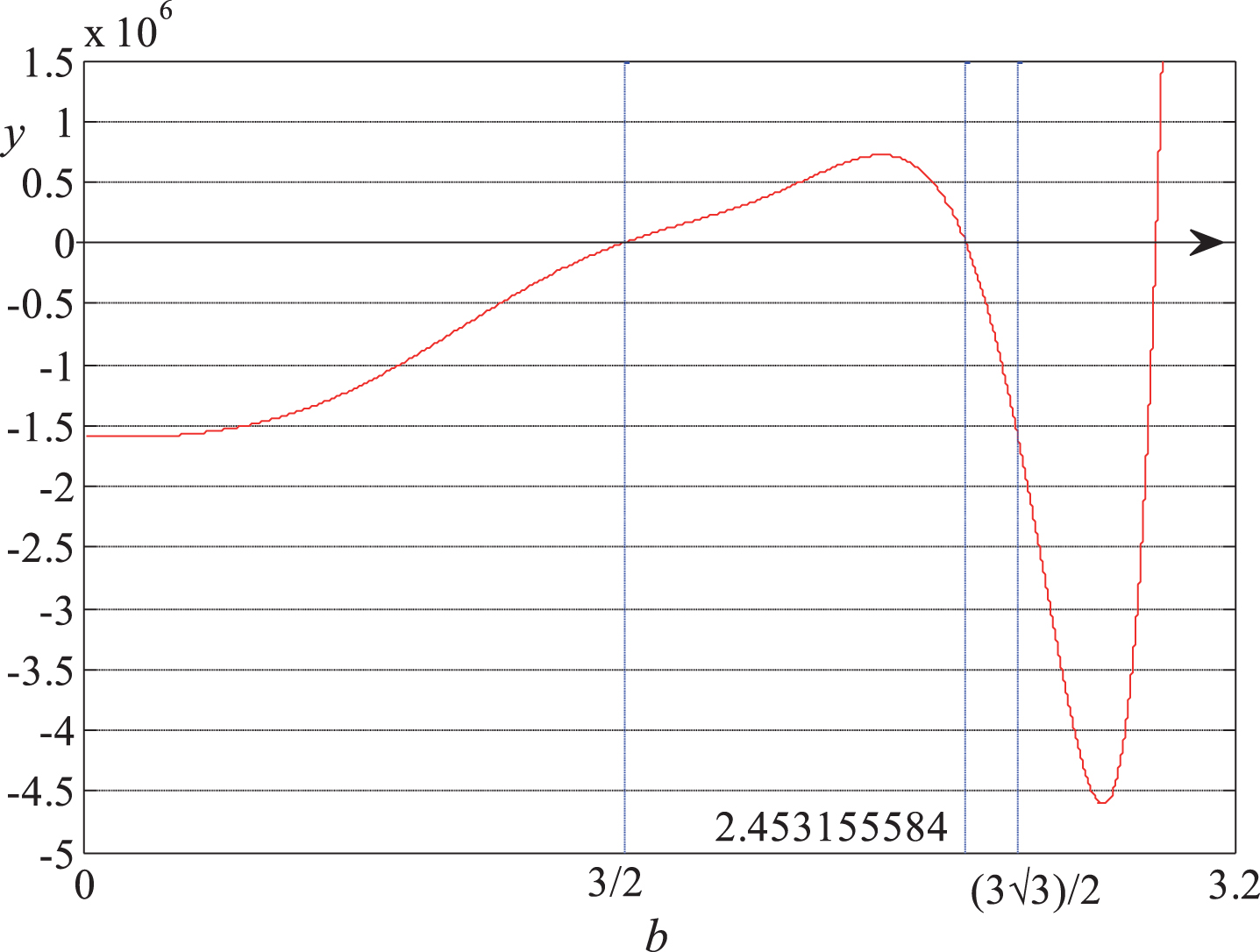
Diagram of the relationship between u and b.

Therefore, if b satisfies condition (6), then f satisfies theorem 1, and is a chaotic map.

Case (II) $J = [- \frac{2 b}{3} \sqrt{- \frac{b}{3 a}}, \frac{2 b}{3} \sqrt{- \frac{b}{3 a}}]$ .

First we show that f : J → J.

In fact, map f is an odd function. Then f : J → J is equal to $f^{2} (x_{5}) \geq f (x_{4}) \Leftrightarrow (b - 3) (2 b + 3)^{2} \leq 0$

that is $b \leq 3$ (7)

If f (x₅) > x₃, we have $b > 3 \sqrt{3} / 2$ (8)

Next, let us show that under condition (3), we can find four points y_i (i = 1, 2, 3, 4) such that $f (y_{3}) = y_{4} \leq y_{1} < f (y_{1}) = y_{2} < y_{3} = f (y_{2})$

Let y₃ = x₃, then y₄ = f (y₃) =0.

Since f (0) =0 < x₃ < f (x₅), then there is a point y₂ ∈ (0, x₅) such that f (y₂) = y₃.

Since f (0) =0 < y₂ < x₅ < x₃ = f (y₂), then there is a point y₁ ∈ (0, y₂) that makes f (y₁) = y₂.

In summary, if b satisfies conditions (7) and (8), that is $3 \sqrt{3} / 2 < b \leq 3$ (9)

Then f satisfies theorem 1, and is a chaotic map.

Using the same approach given in theorem 2, we have theorem3.

Theorem 3. Let polynomial map f have a form $f (x) = ({ax}^{2} + bx) | x + \frac{b}{2 a} | (b > 0)$ (10)

Let J = [0, - b/a] (a < 0) or J = [- b/a, 0] (a > 0), if a and b satisfy $- \frac{\sqrt{3}}{18} \leq \frac{a}{b^{2}} \leq - \frac{\sqrt{3}}{36} (a < 0)$

or $- \frac{\sqrt{3}}{18} \leq - \frac{a}{b^{2}} \leq - \frac{\sqrt{3}}{36} (a > 0)$ then f : J → J satisfies theorem 1. Hence, f is a chaotic map.

Proof. In the following, we just need to prove the case of a < 0 in detail, and the case of a > 0 can be proved similarly.

According to Equation (10), $f (x) = {\begin{matrix} - {ax}^{3} - \frac{3 b}{2} x^{2} - \frac{b^{2}}{2 a} x, x \leq - \frac{b}{2 a} \\ {ax}^{3} + \frac{3 b}{2} x^{2} + \frac{b^{2}}{2 a} x, x > - \frac{b}{2 a} \end{matrix}$

When a < 0, map f have three roots: $x_{1} = 0, x_{2} = - \frac{b}{2 a}, x_{3} = - \frac{b}{a},$

where 0 = x₁ < x₂ < x₃.

Solve f′ (x) =0 and obtain two extreme points:

If $x \leq - \frac{b}{2 a}$ , $x_{4} = \frac{(- 3 + \sqrt{3}) b}{6 a}$ .

If $x > - \frac{b}{2 a}$ , $x_{5} = \frac{(- 3 - \sqrt{3}) b}{6 a}$ .

It is easy to verify that f reaches the maximum value at both points x₄ and x₅, and f (x₄) = f (x₅).

Denote $t_{1} = (- 3 + \sqrt{3}) / 6$ , $t_{2} = (- 3 - \sqrt{3}) / 6$ , then $x_{4} = \frac{b}{a} t_{1}, x_{5} = \frac{b}{a} t_{2}$

If f (x₅) < x₃, that is $a {(\frac{b}{a} t_{2})}^{3} + \frac{3 b}{2} {(\frac{b}{a} t_{2})}^{2} + \frac{b^{2}}{2 a} (\frac{b}{a} t_{2}) \leq - \frac{b}{a}$ $\Leftrightarrow \frac{a}{b^{2}} \leq - \frac{1}{2} (2 t_{2}^{3} + 3 t_{2}^{2} + t_{2}) = - \frac{\sqrt{3}}{36}$ (11)

Then f is a map from [0, - b/a] → & [0, - b/a].

If f (x₄) ≥ x₂, we have $- a {(\frac{b}{a} t_{1})}^{3} - \frac{3 b}{2} {(\frac{b}{a} t_{1})}^{2} - \frac{b^{2}}{2 a} (\frac{b}{a} t_{1}) \geq - \frac{b}{2 a}$ $\Leftrightarrow \frac{a}{b^{2}} \geq 2 t_{1}^{3} + 3 t_{1}^{2} + t_{1} = - \frac{\sqrt{3}}{18}$ (12)

Now, let us show that under condition (12), we can find four points y_i (i = 1, 2, 3, 4) such that $f (y_{3}) = y_{4} \leq y_{1} < f (y_{1}) = y_{2} < y_{3} = f (y_{2})$

Let y₃ = x₂, then y₄ = f (y₃) =0.

If f (x₄) = x₂, set y₂ = x₄, and hence f (y₂) = y₃.

If f (x₄) > x₂ > 0 = f (0), then there is a point y₂ ∈ (0, x₄) that makes f (y₂) = y₃.

Since f (0) =0 < y₂ ≤ x₄ < x₂ = f (y₂), there is a point y₁ ∈ (0, y₂) such that f (y₁) = y₂.

In summary, if a and b satisfy conditions (11) and (12), that is $- \frac{\sqrt{3}}{18} \leq \frac{a}{b^{2}} \leq - \frac{\sqrt{3}}{36}$ (13)

Then f satisfies theorem 1, and is a chaotic map.

3.2 Bifurcation diagram and Lyapunov exponent spectrum

In theorem 2, if 2.453155584 ≤ b ≤ 3, then system (1) is chaotic in the sense of Li-Yorke. Set a = -1. Figure 2(a) and (b) show the bifurcation diagram and Lyapunov exponent spectrum of parameter b in system (1) respectively, where b ∈ [2, 3].

Fig.2

System (1) (a) bifurcation diagram of b; (b) Lyapunov exponent spectrum of b.

Figure 2(a) shows that when 2.453155584 ≤ b ≤ 3, the bifurcation diagram of b displays chaotic characteristics as theorem 2 expects.

In theorem 3, let a = ±1, then if $16 \sqrt{3} \leq b^{2} \leq 12 \sqrt{3}$ , system (10) is chaotic in sense of Li-Yorke. Let b = 1, then if $\sqrt{3} / 36 \leq | a | \leq \sqrt{3} / 18$ , system (10) is chaotic in sense of Li-Yorke.

Figure 3(a) and (b) show the bifurcation diagram and Lyapunov exponent spectrum of parameter b in system (10) respectively, where $b \in [2, 2 \sqrt[4]{27}]$ .

Fig.3

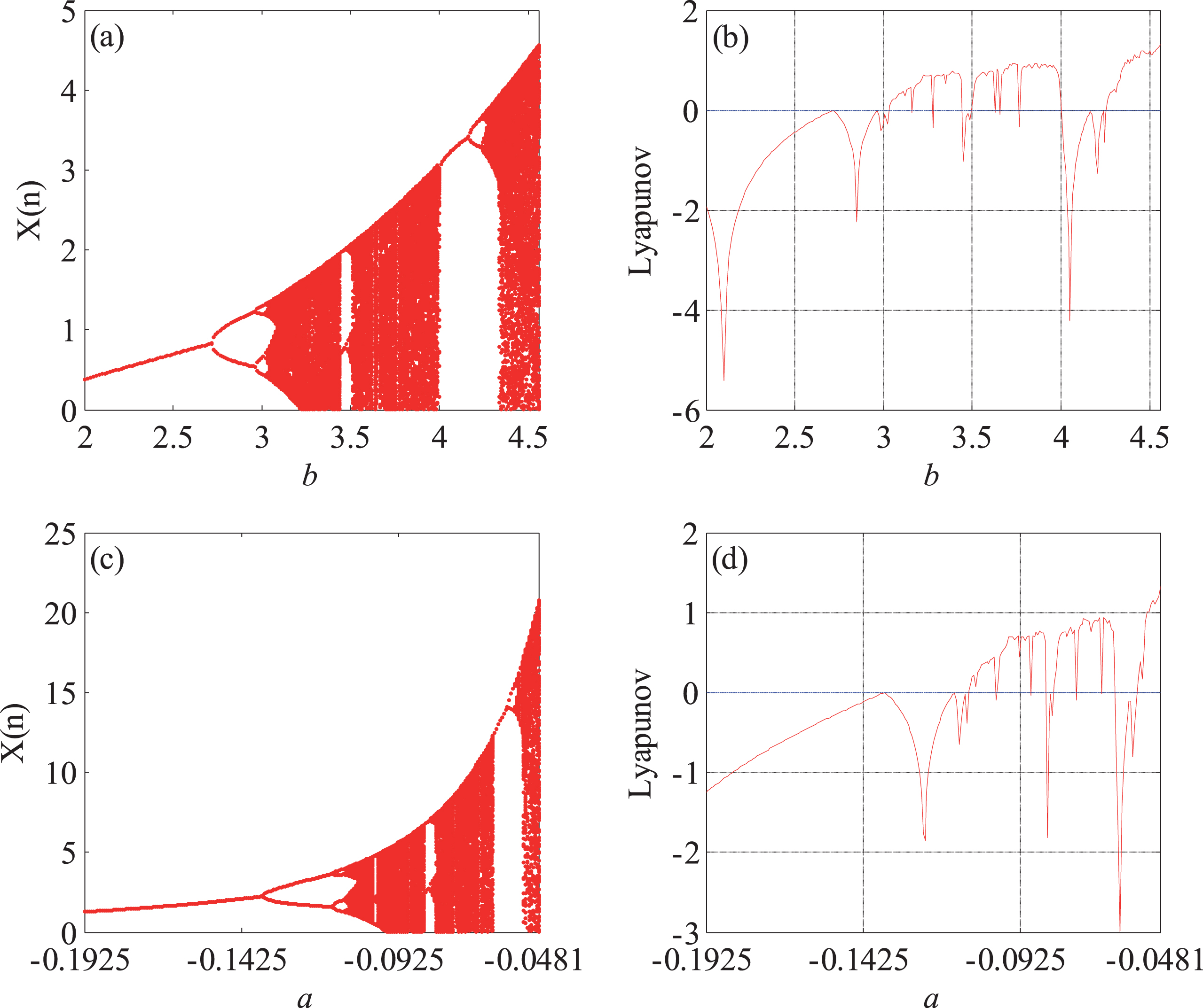
System(10) (a) bifurcation diagram of b; (b) Lyapunov exponent spectrum of b; (c) bifurcation diagram of a; (d) Lyapunov exponent spectrum of a.

Figure 3(a) shows that when $b \in [2, 2 \sqrt[4]{27}]$ , the bifurcation diagram of b displays chaotic characteristics as theorem 3 expects.

Figure 3(c) and (d) show the bifurcation diagram and Lyapunov exponent spectrum of parameter a in system (10) respectively, where $a \in [- \sqrt{3} / 9, - \sqrt{3} / 36]$ .

Figure 3(c) shows when a ∈ $[- \sqrt{3} / 9$ , $- \sqrt{3} / 36]$ , the bifurcation diagram of a displays chaotic characteristics as theorem 3 expects.

4 Complexity analysis of chaotic pseudorandom sequences

4.1 SE algorithm and quantitative method

Based on SE algorithm [18], this subsection analyzes to the complexity of the chaotic pseudorandom sequences generated by the cubic chaotic maps given in section 2. SE can be defined as $se = - \sum_{k = 0}^{N / 2 - 1} P_{k} ln P_{k}, SE = \frac{se}{ln (N / 2)},$ where P_k is relative power spectral density of pseudorandom sequences, N is the length of pseudorandom sequences. The theoretical maximum of SE is 1.

According to the property of the Shannon entropy, the more balanced the power spectrum of the sequence is, the more complex the structure of the power spectrum is. Hence, the larger value of SE means the more complex of sequences. In this paper, the value of SE is used to evaluate the complexity of the chaotic pseudorandom sequences directly, so denote the complexity of sequences as SE complexity in the following analysis.

This paper gives a quantitative method to transform chaotic sequence {Z_n} to the chaotic pseudo-random sequence {Y_n} in base number K, and for instance, K = 2 means the sequence {Y_n} is a binary sequence. The major steps as follows:

Step 1: Assign values to parameters in chaotic systems and initial value, iterate the chaotic system n times, and then obtain chaotic sequence {Z_n}.

Step 2: Start from the 1001th sequence value z₁₀₀₁ of {Z_n}, and then truncate the sequence {X_n} of length N, which means X_i = Z_i+1000, i = 1, 2, ⋯ , N.

Step 3: Define sequence {Y_n} as $Y_{k} = mod (round (\frac{L (X_{k} - X_{min})}{X_{max} - X_{min}}), K)$

where L = 10¹⁵, X_min = min {X_n}, X_max = max {X_n}.

Note: In the following calculation, without special declaration, set K = 2, n = 40000, N = 1000.

4.2 SE complexity analysis

Chaotic systems (1) and (10) will be used to generate chaotic sequences for the SE complexity analysis.

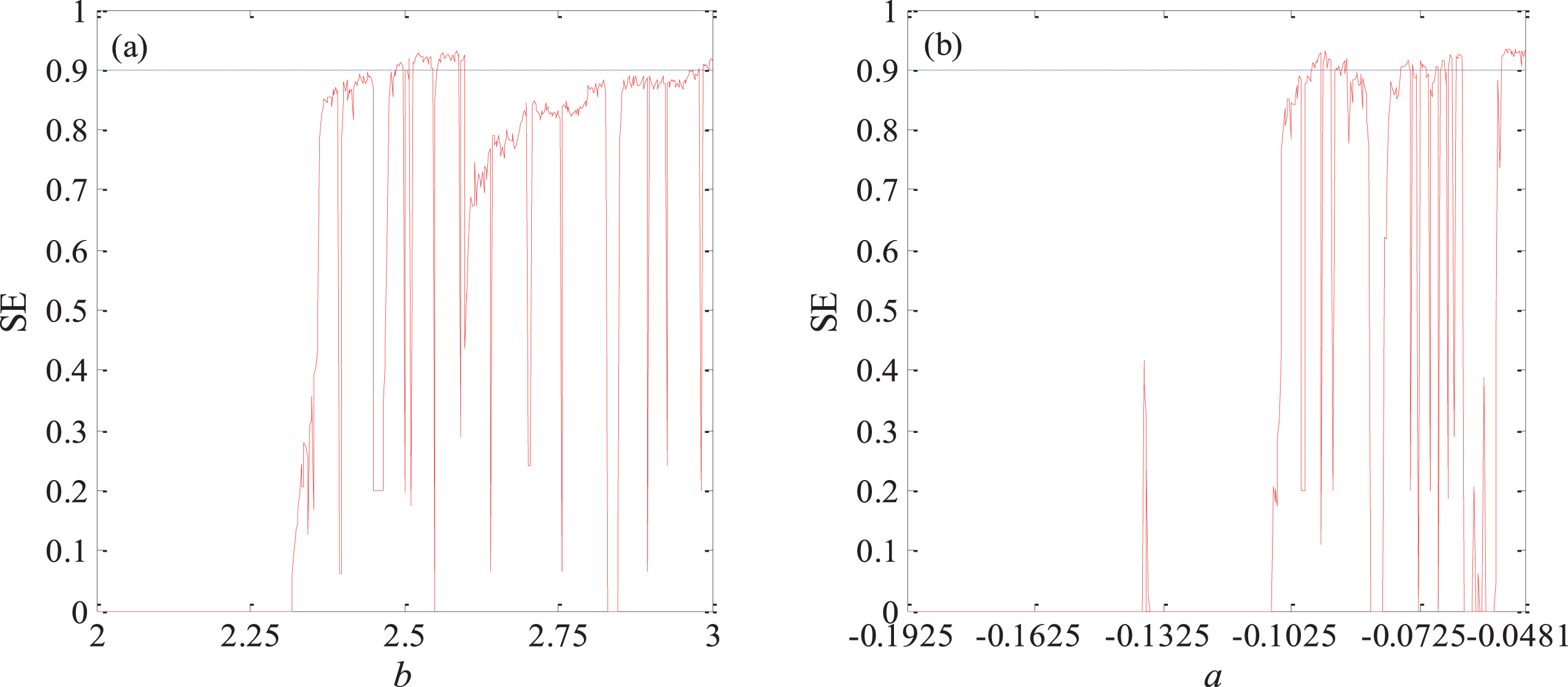
In system (1), let a = -1, b ∈ [2, 3]. In system (10), let b = 1, $a \in [- \sqrt{3} / 9, - \sqrt{3} / 36]$ . Set x₀ = 0.43. The SE complexity of pseudorandom sequences in two systems while parameters vary is shown in Fig. 4(a) and (b).

As shown in Fig. 4, the parameters in system (1) and (10) has little influence to the SE complexity of pseudorandom sequences.

Fig.4

SE of pseudo-random sequence in two system while a or b varies (a) system (1); (b) system (10).

In system (1), let a = -1, b = 3, x₀ ∈ [0, 4]. In system (10), let $a = - \sqrt{3}$ , $b = 3 \sqrt{2}$ , $x_{0} \in [0, \sqrt{6}]$ . The SE complexity of pseudo-random sequences in two systems while initial value x₀ varies is shown in Fig. 5(a) and (b).

As shown in Fig. 5, initial value x₀ has little influence to the SE complexity of pseudorandom sequences.

Fig.5

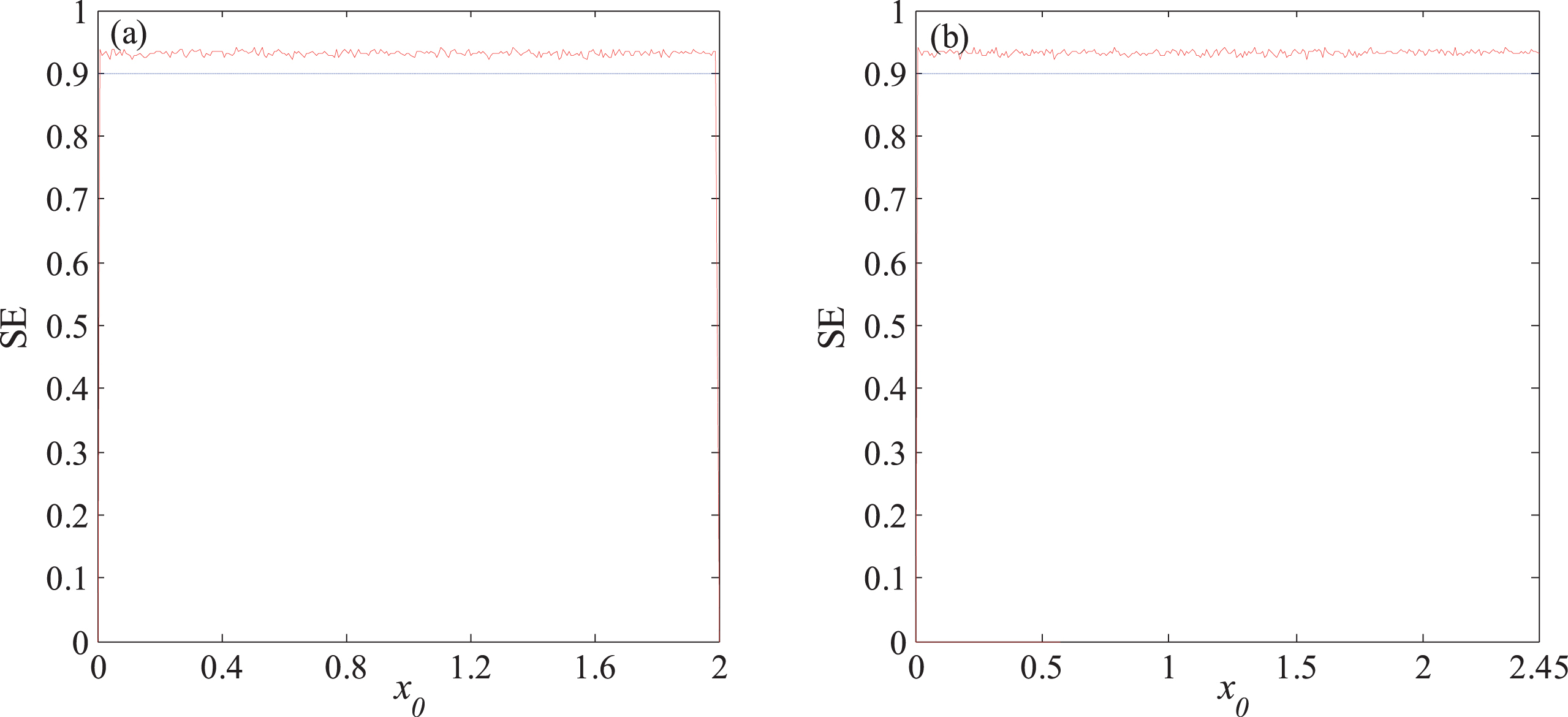
SE of pseudo-random sequence in two system while x₀ varies (a) system (1); (b) system (10).

4.3 SE complexity based on different quantitative methods

The quantitative methods in this paper and in Ref. [18] is different from each other. Now, we further analyze the influence of different quantitative methods to SE complexity of the sequences. The following is discussed from the parameters in systems, number K and length of sequence N.

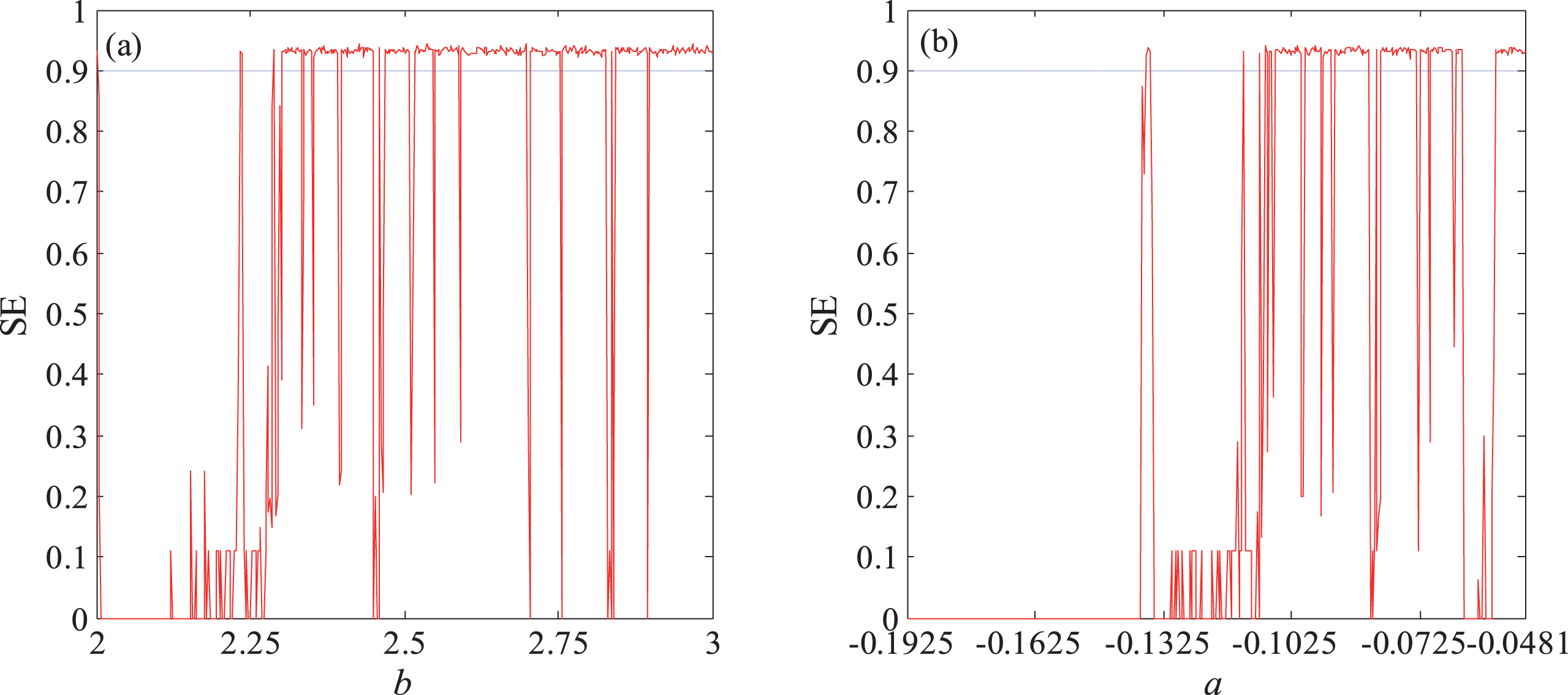
For system (1) and (10), using the quantitative method in Ref. [18], the SE complexity of pseudo-random sequences in two systems while parameters vary is shown in Fig. 6(a) and (b).

Comparing the results in Figs. 4 and 6, we can find that with the same initial conditions, the SE complexity of sequences based on the quantitative method in this paper is generally higher than the SE complexity of sequences based on the quantitative method in Ref. [18]. The results also shows that the different quantitative methods have a significant influence to the SE complexity of sequences.

Fig.6

SE of pseudo-random sequence in two system while a or b varies (a) system (1); (b) system (10).

Furthermore, we analyze the influence of number K and length of sequence N to SE complexity of sequences while other conditions keep same. In system (1), let a = -1, b = 3. In system (10), let a = -0.072, b = 1. Set x₀ = 0.43.

Figure 7(a) and (b) show the SE complexity of sequences based on the quantitative method in this paper while parameters K or N varies. Figure 7(c) and (d) show SE complexity of sequences based on the quantitative method in Ref. [18] while parameters K or N varies.

Fig.7

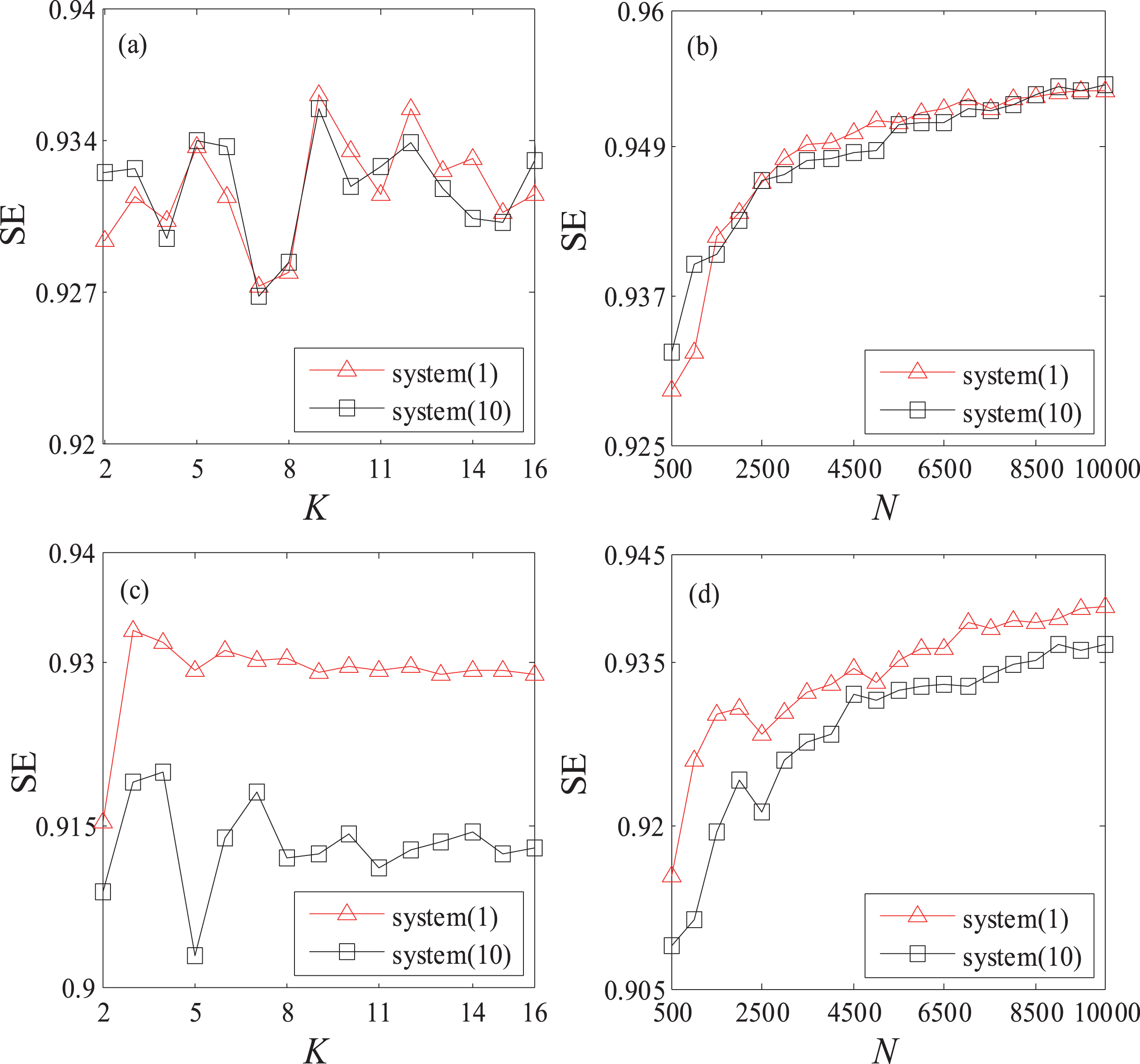
SE of pseudo-random sequences in different chaotic systems (a), (c) K; (b), (d) N.

As shown in Fig. 7(a) and (b), based on the on the quantitative method in this paper, the SE complexity of pseudo-random sequences generated by system (1) and (10) have no significant difference. However, as shown in Fig. 7(a) and (b), based on the on the quantitative method in Ref. [18], the SE complexity of pseudo-random sequences generated by system (1) is significantly higher than the SE complexity of pseudo-random sequences generated by system (10). Hence, the results also show that the different quantitative methods have a significant influence to the SE complexity of sequences.

5 Conclusion

Firstly, based on Li-Yorke’s chaos criterion, this paper sets up two new chaos criterions on cubic polynomial maps. It is needed to note that the purposed cubic polynomial maps are both limited in special form. Hence, more work should be carried out to chaos discriminant conditions for general cubic polynomial maps. The numerical simulations of the bifurcation diagram and Lyapunov exponent spectrum are carried out to show that the theorems purposed in this paper can be easily used and verified.

Secondly, this paper analyze the complexity of the pseudorandom sequences generated by the given cubic chaotic maps. The numerical results shows that initial values and parameters in systems have little influence to the SE complexity of sequences. Furthermore, the comparative results of SE complexity of sequences based on different quantitative methods show that the quantitative method has a significant influence to the SE complexity of sequences. And it is showed that the quantitative method in this paper makes the pseudo-random sequences have a better SE complexity comparing with the Ref. [18].

Nonetheless, the complexity of chaotic systems cannot been only evaluated by SE complexity. More performance evaluation is required to gain the more accurate conclusions.

Footnotes

Acknowledgments

The work was supported by the Fundamental Research Funds for the Central Universities of China (Grant Nos. 06108236).

References

T.Y.

and Yorke

J.A.

Period three impiles chaos, Am. Math. Mon 82(10) (1975), 985–992.

Liu

, Li

P.Y.

, et al., Construction of a class of chaos systems with Markov properties, Acta Phys. Sin. 62(17) (2013), 116–121.

, Li

Z.J.

and Chen

X.X.

Dynamics analysis and circuit implementation of fractional-order Chua’s system with negative parameters, Acta Phys. Sin 66(23) (2017), 60–69.

Wang

C.F.

and Ding

SM4 key scheme algorithm based on chaotic system, Acta Phys. Sin 66(2) (2017), 76–84.

Zhang

, Shi

Y.M.

and Chen

G.R.

Constructing chaotic polynomial maps, Int. J. Bifurcation and Chaos 19(2) (2009), 531–543.

Zhang

Chaotic polynomial maps, Int. J. Bifurcation and Chaos 26(8) (2016), 1650131.

Zang

H.Y.

and Chai

H.Y.

Homogenization and entropy analysis of a quadratic polynomial chaotic system, Acta Phys. Sin 65(3) (2016), 64–70.

Zhou

H.L.

and Song

E.B.

Discrimination of the 3-periodic points of a quadratic polynomial’, Journal of Sichuan University 46(3) (2009), 561–564.

Wang

W.B.

, Wang

X.D.

, et al., Construction of chaos polynomial family, Electric Machines & Control 13(a01) (2009), 109–112.

10.

Yang

X.P.

, Min

L.Q.

and Wang

A cubic map chaos criterion theorem with applications in generalized synchronization based pseudorandom number generator and image encryption, Chaos 25(5) (2015), 0531041–9.

11.

Wang

, Liu

, et al., A pseudorandom number generator based on piecewise logistic map, Nonlinear Dyn. 83(4) (2016), 2373–2391.

12.

Dastgheib

M.A.

and Farhang

A digital pseudo-random number generator based on sawtooth chaotic map with a guaranteed enhanced period, Nonlinear Dyn 89(1) (2017), 1–10.

13.

Liu

L.F.

, Miao

S.X.

, et al., N-phase logistic chaotic sequence and its application for image encryption, IET Signal Processing 10(9) (2017), 1096–1104.

14.

S.B.

, Sun

K.H.

and Wang

H.H.

Modified multiscale permutation entropy algorithm and its application for multiscroll chaotic systems, Complexity 21(5) (2016), 52–58.

15.

Dang

T.S.

, Palit

S.K.

, et al., Complexity and synchronization in stochastic chaotic systems, European Physical Journal Special Topics 225(1) (2016), 159–170.

16.

Chen

X.J.

A New Complexity Metric of Chaotic Pseudorandom Sequences Based on Fuzzy Entropy, Journal of Electronics & Information Technology 33(5) (2011), 1198–1203.

17.

Liang

D.Q.

, Chen

Z.G.

and Deng

X.H.

Analysis of Chaotic Sequence Complexity Based on Wavelet Packet Energy Entropy, Acta Electronica Sinica 43(10) (2015), 1971–1977.

18.

Sun

K.H.

and He

S.B.

et al., Complexity analysis of chaotic pseudo-random sequences based on spectral entropy algorithm, Acta Phys. Sinica. 62(1) (2013), 0105011–8.