Towards implementing defect prediction in the software development process

Abstract

Defect prediction is a method of identifying possible locations of software defects without testing. Software tests can be laborious and costly thus one may expect defect prediction to be a first class citizen in software engineering. Nonetheless, the industry apparently does not see it that way as the level of practical usages is limited. The study describes the possible reasons of the low adoption and suggests a number of improvements for defect prediction, including a confusion matrix-based model for assessing the costs and gains. The improvements are designed to increase the level of practitioners acceptance of defect prediction by removing the recognized by authors implementation obstacles. The obtained predictors showed acceptable performance. The results were processed through the suggested model for assessing the costs and gains and showed the potential of significant benefits, i.e. up to 90% of the overall cost of the considered test activities.

Keywords

software metrics software development process defect prediction re–open prediction predicting feature defectiveness defect prediction economy

1 Introduction

Defect prediction is a technique used to predict faultiness of a given software artefact expressed in terms of defects. It could be the number of defects or binary information indicating whether the artefact is defect free or not. Such a technique seems to be very useful in the software development process. If one knew which artefacts are defect free, one could save efforts related to testing them. The software tests are often estimated for up to 50% of the costs of the whole software development (Kettunen et al. [1]). Therefore, such savings should be substantial, but surprisingly there is few evidence of defect prediction implementations in real life software development processes and all of the few exceptions most likely were conducted in close collaboration with defect prediction researchers ([2 –4]), i.e. the companies were not able to implement the prediction by their own. Moreover, there are reports from research departments of software vendors with complaints regarding challenges related to convincing project managers to start using the defect prediction models (Weyuker and Ostrand [5]). One may wonder why as one of the earliest defect prediction models was suggested in the 70’ (Halstead [6]) and since then it is intensively investigated by many researchers (Hall et al. [7] or Jureczko and Madeyski [8]) and the prediction results are encouraging. According to Hall et al. [7] the model precision is usually close to 0.65 and after calibration it can be much better (e.g. up to 0.97 after performing feature selection and choosing optimal classifier as reported by Shivaji et al. [9]). We considered a survey aiming at characterizing the reasons of low adoption of the technique. Unfortunately, preliminary interviews with people deciding about the shape of development process show very limited understanding of the concept of defect prediction (there was no case where the defect prediction was even considered). Thus a survey might be of low value. It makes us thinking about the possibility of launching defect prediction program in our own environments and we faced challenges related to discrepancies between defect prediction assumptions and the real life software development processes. We identified challenges that in our opinion should be solved before recommending defect prediction. Let us present the issues and our concerns.

Issue 1: the mapping of defects to the prediction unit of analysis. According to Hall et al. [7] most of the defect prediction models are focused on files and classes. The files and classes pointed out by the model are recommended for code review or special care during testing (Weyuker et al. [10]), in the case of the aforementioned artefacts that would be unit tests. Let us first consider what is meant by the fact that a class or file is defective in the context of defect prediction. Most of the researchers (e.g. [11, 12]) identify the defects in files and classes using issue tracking systems or commit messages. The procedure is usually as follows. Defect reports are extracted from the issue tracking system and subsequently from each defect report its identifier is extracted. Then the comments in the project’s version control system are scanned for occurrences of the aforementioned identifier. When there is a match, all classes or files that were modified in the identified version control commit are marked to be defective. In consequence, there can be a defect report regarding malfunction on a system business level, visible to the end–users and a number of classes that were changed during defect fixing. When the defect root cause comes from a technical flaw of the implementation (e.g. error in sorting algorithm) there is nothing wrong with that. Unfortunately there is always a fraction of defects with the root cause outside the source code (e.g. misinterpretation of requirements). Such defects typically result in a number of changes done in coupled classes. Some of the changes address more or less directly the defect whereas others are side effect adjustments in the coupled code. In order to better illustrate this case let us present an example. One of the commonly investigated projects with respect to defect prediction is JEdit e.g. in [13, 14]. Among others, there is a defect report with number 2739: ‘Indentation of Javascript embedded in HTML is broken’¹. It has been fixed in revision 8093 by introducing changes to 5 files. One of them is JEditTextArea.java where one line was changed, that is:

indent = buffer.isElectricKey(ch); to indent = buffer.isElectricKey(ch, caretLine);

An additional parameter is passed to the isElectricKey method. Does it mean that the method was defective before the change? The answer is not clear, specifically because the ‘buffer’ class (i.e. JEditBuffer) was changed in the same commit. We ended up with a real defect mapped into changes in the source code that really solve it which is not exactly the same as a set of defective classes. Nonetheless, the prediction model is trained to predict them as defective, whereas in fact we are not sure about their real status. Furthermore, it is hardly possible that a unit test or code review of the JEditTextArea.java file will result in a corrective action regarding the isElectricKey method, as without the broader context that comes from the defect report, it is not clear that there is something wrong with the method call. Defect prediction output pointing at the JEditTextArea.java would be useless for a practitioner despite being correct. Furthermore, automatic identification of technical issues is the goal of static code analysis which already have good tool support e.g. FindBugs™², SonarQube™³. Not all defects are similar to the one described above, but neither it is an exceptional corner case.

Issue 2: no clear definition of defect prediction data collection program. Another possible issue related to the practical application of defect prediction regards defects distribution, or more specifically, defect reports distribution. The researchers do not report if their data resulting from uniform tests of the whole system. Possibly, the opposite is true since it is recommended to focus test efforts on new and changed functionalities. Namely, it is possible that the ‘prediction’ shows which parts of the system were tested. In other words, the following scenario is plausible. Before the release, some of the features (the new or changed ones) are intensively tested and in consequence a number of defects are reported whereas the rest of the systems goes only through light regression tests that do not result in many additional defect reports. The identified defects are used to train the prediction model. However, the tests were conducted in such a way that the vast majority of defects were identified in certain parts of the system. In consequence, the model is adjusted to the design flaws and development history of the tested parts of the system instead of to the defects. Whereas the theory behind software metrics based defect prediction suggests that some design flaws (e.g. high coupling) increase the possibility of committing a defect, and thus the prediction model should recognize those design flaws. A similar scenario is also possible for post–release defects as the customer may follow the same principles during validation (i.e. focus on new and changed functionalities) or simply train users in only what is new in a given release. The scope of conducted tests should not be ignored in the evaluation of defect prediction efficiency. Claiming that defect prediction works for entire systems when only half of it is considered for the quality assurance activities may misleadingly increase prediction efficiency. What is the value of prediction precision equal to 0.97 when half of the system was not tested at all and the predictor just learned the rule behind excluding certain software artefacts from testing?

Issue 3: no estimation of return of investment. Defect prediction requires a software measurement program and thus does not come for free. Since some investments must be made, it is crucial to assess the future benefits that may come from using defect prediction and confront them with the costs. Fortunately, the costs of metrics collection have already been analyzed e.g. [15], but what the benefits look like is not so clear. There are two concepts of employing defect prediction in software development. Weyuker et al. [10] suggested to use the model output as a trigger for additional tests and code reviews which should result in improving software quality and hence reduce the number of post–release defects. Briand et al. [16] pointed out the possibility of savings regarding not testing artefacts that were predicted to be defect free. This work is focused on the latter as detailed empirical data (which unfortunately is unavailable for us) is needed for the evaluation of the first one ([17]). We suggest a method of assessing the benefits (and costs) of not testing software artefacts that presumably are defect free.

Issue 4: poor tool support. Developing tools for industry is not a something that can be done as a part of research paper. Nonetheless, it is a very important obstacle that may not be ignored. Yang et al. [18] reported, that industrial practitioners are more interested in in the interpretations and follow-up that occur after prediction than in just the mining itself. Following the same this work suggests a number of changes to the design of defect prediction in order to address as many of the aforementioned issues as possible.

The usefulness of the redefined defect prediction is tested on two open–source projects using the suggested model for assessing costs and gains. The rest of this paper is organized as follows. The suggested approach to defect prediction as well as the method of assessing prediction gains and cost are described in the next section. The Section 3 contains the detailed description of our empirical investigation aimed at predicting defects re–opens. Threats to validity are discussed in Section 4. Related studies concerning re–opens prediction and the evaluation of costs and gains of defect prediction are presented in Section 5. The conclusions, contributions and plans for future research are discussed in Section 6.

2 Proposed approach for implementing and assessing defect prediction

The goal of this work is to redesign the defect prediction by suggesting approaches that avoid or resolve the issues mentioned in introduction. We conducted an empirical experiment that employs the defect prediction in such a way that makes the practical application of prediction outcomes straightforward and minimizes the possibility of misleading evaluation of prediction effects. Additionally, we suggest a model for assessment of the defect prediction application costs and benefits.

2.1 The place of defect prediction in software development

The defect prediction models that use larger artefacts as the unit of analysis seem to be more handy as it is easier to map them to system level requirements and due to the size, they come with a broader context. Hall and Fenton [7] reported modules which unfortunately are vaguely defined. We believe that the usefulness of such models depends on what in fact the module is and what the software development process looks like. Nonetheless, in our opinion the larger artefacts are a promising direction and therefore constitute our primary concern.

Let us consider two scenarios that commonly emerge in software development, i.e. implementation of a new feature and correction of a defect. Both of them can be very complex, but for our considerations we can limit them to several crucial steps. In the case of the new feature, there is the writing of the source code; afterwards the tests should be conducted and then, according to the tests results, the feature is released or goes back to the development team for further improvements and tests, which creates a loop in the process. Eventually, the feature is released and in consequence the end users start to use it. Unfortunately, the tests do not guarantee correctness and it is possible that after the release some hidden defect will emerge. Such situations create losses for the software vendor regarding efforts contributed to defect fixing as well as ruining the brand image.

The second scenario, i.e. defect correction (commonly called bug fixing) is in fact very similar. When a new defect report appears, some source code must be written or changed, subsequently the defect correction should be tested and according to the test result, released or re–implemented. Due to the similarities, a single activity diagram can be used to render both of them, that is Fig. 1.

Fig.1

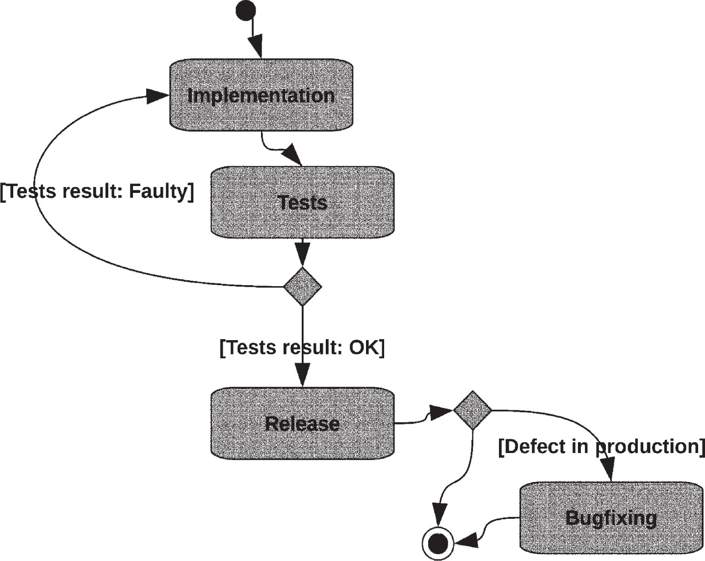
Software implementation: new features & bugfixing.

According to the Fig. 1 there is a saving possibility. By knowing upfront that something is implemented correctly we can skip the tests without harm to the system quality (in some cases such simplification may be impossible due to regulations, e.g. development of medical devices. Unfortunately, this is knowledge the practitioners do not posses. It is only possible to predict the correctness of implementation and this is what the defect prediction models are about. When considering the usage of defect prediction the software implementation diagram should be extended as it is presented on Fig. 2. The defect prediction is used to decide whether tests should be conducted. Software vendors are not eager to plan the tests according to prediction results, i.e. to chose upfront to not test some of the artefacts. However, when there are not enough resources to meet the deadline some hard decisions must be made. When postponing the deadline is not an option the only alternative is to skip some of the tests. The number of skipped test will presumably depend on the available resources whereas defect prediction will only be used to prioritize them. Nonetheless, the available resources are not a feature of defect prediction and thus should not be considered as a factor in defect prediction costs and gains assessment. This is a simplification that deviates from the real resources allocation, but without significantly worsening the estimation quality of the expected costs and gains which is introduced in the next subsection. The estimation is acceptable since after testing all artifacts marked as defective we can do more tests i.e. trading some of the saved resources for lower risk of releasing a defect.

Fig.2

Software implementation with defect prediction. In brackets there are probabilities and efforts used in the discussed in next subsection model.

There are two different defect prediction units of analysis that are compatible with the flow presented on Fig. 2: features and defect fixes and in order to have an easy commercial implementation we suggest to not use other ones. When the unit of analysis is smaller (e.g. the commonly investigated files or classes) it is challenging to define a set of actions that should be executed in response to the prediction results. The file or class level artefact are covered by unit tests which are usually automated and created not only to detect defects but also to prevent regression, enable safe refactorings and sometimes as a low level documentation, hence optimizing the number of unit tests according to prediction outcome may have unexpected consequences and makes the impact of defect prediction application hardly possible to evaluate. Furthermore, even the two suggested units of analysis may create complications. A defect fix which is the object of re–opens prediction is usually small and thus we do not expect significant deviations from the presented flows. However, features differ in size and not always are autonomous. When a project is developed in phases and each of the phases spans a number of possibly tightly coupled which each other features it might be not reasonable to analyze each feature in separation as there is considerable risk of introducing defect in feature B when developing feature A. We can consider a feature autonomous for the sake of defect prediction only when regression in other features can be guarded without manual tests and thus there (in the other features) is no significant test effort during development of the autonomous feature. Otherwise the scope of tests executed during verification of a feature exceeds the boundaries of the feature which makes reasonable releasing features in bulks to reduce the number of repetitions of the same test scenarios and dramatically changes the flow. As a consequence, the suggested in this work solution is applicable to iterative processes that are driven by features (e.g. Scrum) and take care of modularity (e.g. micro services architecture). Application in other processes (e.g. waterfall) or designs (e.g. monolith) may not work as expected.

2.2 Model for defect prediction expected costs and gains assessment

The defect predictions are not perfect. Sometimes, the prediction is wrong and the low quality source code that would be reported during tests may be released and hence there is a loss for the software vendor. Therefore, it is not obvious that the process depicted on Fig. 2 is more cost–effective. Let us consider four different scenarios in order to evaluate the overall effect of employing a defect prediction model. The intention of the evaluation is to show the gain (or loss) in comparison to a baseline which is testing all software artefacts.

Scenario faulty&faulty (implementation: faulty, prediction: faulty). The artefacts are tested and thus there is no deviation from the baseline.

Scenario faulty&ok (implementation: faulty, prediction: OK). According to the prediction results the software artefacts are not tested, but in fact they are incorrect and thus should be tested and corrected. Not all defects are discovered during tests, thus the testing effectiveness should be considered in this scenario. In consequence, there is a loss related to releasing system with defects.

Scenario ok&faulty (implementation: OK, prediction: faulty). The artefacts are tested and thus there is no deviation from the baseline.

Scenario ok&ok (implementation: OK, prediction: OK). The artefacts are correct and are not tested. Thus, there are savings that come from skipping the tests.

In order to render the evaluation in a more formal way, let us define: I_f – implementation not correct (faulty), I_ok – implementation correct, C_pr – post–release cost connected with releasing a defective software artefact, C_t – costs of testing a software artefact, Pr_ok – prediction result: implementation is ok, e – testing effectiveness, where 0 ≤ e ≤ 1 and e = 1 represents detecting all defects in the inspected software artefacts, G – expected gain (or loss when G is below 0) of prediction model application for certain artefact, i.e. the gain that comes from employing the model in software development with respect to a certain artefact, TG – total gain of prediction model application, i.e. the sum of values of G calculated for all artefacts, P (x) – probability of x, we are using also conditional probabilities, $\bar{x}$ – average value of x, n – number of software artefacts. $G = P (I_{ok}) * P (\Pr_{ok} | I_{ok}) * C_{t} - P (I_{f}) * P (\Pr_{ok} | I_{f}) * (e * C_{pr} - C_{t})$ (1) The value of G equals the difference between the gain that comes from scenario ok&ok and loss from scenario faulty&ok and is expressed in the same unit as C_pr and C_t which can be man–days as well as money. The scenario ok&ok is the probability of the occurrence of two random events i.e. correct implementation and defect prediction outcome stating that the implementation is correct, multiplied by the costs of testing. In other words it is the expected saving from not testing the correctly implemented features. The scenario faulty&ok is the probability of two random events, i.e. faulty implementation and prediction claiming that the very same functionality is defect free, multiplied by the expected cost of releasing defective functionality. The cost of releasing defective functionality is reduced by the value of costs of the tests, since according to prediction outcome tests are not conducted. In other words, the scenario represents the expected loss being a result of skipping tests of defective functionality because of encouraging prediction results.

The equation can be reformulated in a more compact form when assuming that P (gain) = P (I_ok) * P (Pr_ok|I_ok) and P (loss) = P (I_f) * P (Pr_ok|I_f): $G = P (gain) * C_{t} P (loss) * (e * C_{pr} - C_{t})$ (2) Unfortunately even the compact form is not handy when calculating TG since it would be necessary to know the value of G for each of the artefact that goes through the defect prediction process. And this is knowledge we cannot expect in a real life software development process. In order to make it applicable in practice, we need a simplifying assumption, i.e. the testing cost is not correlated with neither actual implementation status (correct, not correct) nor defect prediction results (the two later ones should be correlated with each other). With the aforementioned assumption, TG can be calculated using the following formula: $TG = n * (\bar{P (gain)} * \bar{C_{t}} - \bar{P (loss)} * (e * \bar{C_{pr}} - \bar{C_{t}}))$ (3) Please note that the $\bar{P (gain)}$ and $\bar{P (loss)}$ can be estimated using confusion matrix: $\bar{P (gain)} = \frac{artefacts in scenario ok & ok}{n}$ (4) $\bar{P (loss)} = \frac{items in scenario faulty & ok}{n}$ (5) The C_pr, C_t as well as testing effectiveness can be company or project specific. Hence, we advise to estimate them using company historical data or expert opinion. We recommend to overestimate test effectiveness and the relation of C_pr to C_t when using the Equation 3 in making decision about using defect prediction. Such estimations will lead to underestimating the TG and as a consequence the defect prediction results should not be worse than expected. We followed the recommendation in the experiments presented in next section. Test effectiveness represents the proportion of defects identified during tests. When is very low, the majority of defects pass tests and hence testing is not economically justified regardless of the quality of prediction. When C_pr is much bigger than C_t we set high expectations for the defect prediction as releasing a defect becomes relatively expensive while tests are cheap.

3 Experiment

We see two different defect prediction units of analysis that corresponds well with the presented in previous section considerations, those are features and defect “re-opens”. In this section we are applying defect prediction to the later ones. The purpose of the experiment was to predict whether and in what conditions a bug which was resolved can be “re–opened” in the future. The experiment is based on data collected from two open–source projects: Flume and Oozie.

3.1 Experiments design

In order to perform classification we created an application using WEKA that is a powerful tool for data mining. It gives a possibility to classify data using various classification methods, feature selection, visualize obtained classification results (e.g. decision trees), etc.

To validate the performance of a prediction we used 10–fold cross–validation method (CV). After splitting data into training and test sets, in the next step a feature selection on training set was performed for each fold. Thanks to that we could select a subset of features which are the most appropriate for predicting whether a bug can reappear in the future. In the feature selection process we used Best-First Search algorithm. This algorithm connects advantages of breadth–first searching (prevents the situation of finding a ‘dead end’) and depth of the first search (finding solution without examining every ‘competitive’ resolution). Generally, the algorithm is used for searching the graph, but in our situation it is suitable too. The Best–First Search algorithm is based on choosing every step in this option, for which estimation of evaluation function is the best. In our case Best–First searches the space of feature subsets by greedy hill-climbing augmented with a backtracking facility. As evaluating function we chose the ‘ClassifierSubsetEval’ function. It evaluates attribute subsets on training data and uses a classifier to estimate the ‘merit’ of a set of attributes. We used J48 classifier as an evaluator.

The next step was data classification. Number of instances belonging to specific classes: “Bad” or “Good” in predicting if bug can be re–opened (“Bad” means, that bug can be re–opened and “Good” that it will probably not happen) was imbalanced. In initial dataset, a number of instances with “Good” value for “Re–opened” attribute was much more numerous than those with “Bad” value in both Flume and Oozie projects. To solve this problem we used SMOTE (Synthetic Minority Over–sampling Technique) [19].

After including SMOTE, a classification method was chosen. According to [7] among the most frequently used in defect prediction are Decision Trees, Regression-based and Bayesian approaches. Hence, we decided to employ two from each of those categories: J48graft, BFTree, Logistic, ClassificationViaRegression, BayesNet and NaiveBayesSimple. with default classifiers parameters values, only the threshold value has been raised to 0.85 to reflect the loss function which in our case is asymmetric. We recommend using a value that is related to the ratio of the cost of releasing defect (e * C_pr - C_t) to the cost of testing (C_t).

To evaluate the obtained results we used Recall (probability of correct classification of a faulty artefact) and Precision (proportion of correctly predicted faulty modules amongst all modules classified as faulty).

3.2 Data collection

We investigated two open-source projects: Oozie and Flume with respect to predicting defect re–opens. Oozie is a server–based workflow scheduling and coordination system to manage data processing jobs for Apache Hadoop. Oozie has been developed since August 2011 and by April 2017 it had 191,960 lines of code (the aforementioned dates provide the data collection time interval). More information about this project is available on http://oozie.apache.org/. The second project, Flume, is a distributed, reliable, and highly available service for efficiently collecting, aggregating, and moving large amounts of log data. It has a simple and flexible architecture based on streaming data flows. Flume is robust and fault tolerant with tuneable reliability mechanisms It uses a simple extensible data model that allows for online analytic application (http://flume.apache.org/). Project has been developed since June 2010 and has 93,429 lines of code (April 2017). Information about issues related with both projects can be found at https://issues.apache.org/jira/.

The two projects were chosen due to their rich history about defects including re–opens, i.e. they have 1,087 bugs and 77 bugs which have (or had) status “Re–opened” (Flume) and 1,484 bugs and 429 have a “Re–opened” status (Oozie). To collect data about defects we used an application developed at Wroclaw University of Science and Technology – QualitySpy [20]. It is a tool for collecting data about the history of issues in software projects stored in issue tracking systems (e.g. Atlassian JIRA) and other software development systems. More information about QualitySpy can be found on https://opendce.atlassian.net/wiki/spaces/QS. Using this tool we collected 18 attributes – 17 independent variables and the object of prediction, i.e. whether a defect has been re–opened:

created – date of issue creation,

resolved – date of issue first resolution,

fixing duration – time from issue creation to first resolution (in days),

resolution day of week – day of week of the issue first resolution,

resolution day of month – day of month of the issue first resolution,

resolution day of year – day of year of the issue first resolution,

resolution month – day of month of the issue first resolution,

resolution hour – hour of day of the issue first resolution,

component in which bug was found,

environment in which bug occurred (operating system, Java version, etc.),

initial priority – one of the following: trivial, minor, major, critical, blocker,

advancement of project – days between creation of the first issue in project and current issue creation,

number of defects reported by reporter – number of defects reported by the reporter of current issue before the current issue,

number of defects resolved by assignee – number of defects resolved by person assigned to current issue before current issue resolution,

number of changes registered in the issue tracking system before current issue,

number of comments in the issue tracking system, in the current issue,

number of changes of the assignee before issue resolution date,

re–opened – if the issue was re–opened after the first resolution.

Most of selected attributes was suggested by [21]. We investigated attributes which can be divided into 4 categories: work habits (created, resolved, attributes regarding resolution time), bug report (component, environment, advancement of project, initial priority), bug fix (fixing duration, re–open, number of changes, number of comments), people (reported by reporter, resolved by assignee, assignee changes). Attributes from this categories can be use to check what have the biggest influence on predicting if bug can be re–opened in future. The collected data were published online⁴.

3.2.1 Experiment result

In this section we want to put results of our research about predicting whether bug can be re–opened in future. Results obtained for the Flume project are presented in Table 1 and for Oozie in Table 2.

Table 1
Classification results for “Re–opens” prediction in Flume project

Classifier $_{FN}^{TP}$ $_{TN}^{FP}$ Recall Precision TG [h] % of savings

J48graft 44 33 .936 .571 1958 90.1

3 1006

BFTree 44 33 .846 .571 1858 85.5

8 1001

Logistic 58 19 .274 .753 –1062 –48.9

154 855

ClassificationViaRegr. 25 52 .735 .325 1838 84.6

9 1000

BayesNet 58 19 .958 .782 1959 89.3

3 1006

NaiveBayesSimple 63 14 .178 .791 –2882 –133.9

245 764

Classifier	$_{FN}^{TP}$	$_{TN}^{FP}$	Recall	Precision	TG [h]	% of savings
J48graft	44	33	.936	.571	1958	90.1
	3	1006
BFTree	44	33	.846	.571	1858	85.5
	8	1001
Logistic	58	19	.274	.753	–1062	–48.9
	154	855
ClassificationViaRegr.	25	52	.735	.325	1838	84.6
	9	1000
BayesNet	58	19	.958	.782	1959	89.3
	3	1006
NaiveBayesSimple	63	14	.178	.791	–2882	–133.9
	245	764

Table 2

Classification results for “Re–opens” prediction in Oozie project

Classifier	$_{FN}^{TP}$	$_{TN}^{FP}$	Recall	Precision	TG [h]	% of savings
J48graft	177	252	.983	.413	2050	69.0
	3	1052
BFTree	252	177	.966	.587	1930	65.0
	9	1046
Logistic	375	54	.658	.874	-1790	-60.0
	195	860
ClassificationViaRegr.	67	362	.985	.156	2090	70.4
	1	1054
BayesNet	369	60	.979	.860	1950	65.7
	8	1047
NaiveBayesSimple	375	54	.658	.874	-1790	-60.0
	195	860

Ten–fold cross validation with the SMOTE technique for data balancing was used and resulted in satisfactory outcomes, i.e. Recall up to 0.982 and Precision up to 0.997 in the Flume project and Recall up to 0.946 and Precision up to 0.999 in the Oozie project. Nonetheless, the confusion matrix is the most interesting outcome with respect to the defect prediction costs and gains assessment. It shows in the case of the Flume project that there were 1009 correctly resolved defects (n_ok = 1009) and 77 re–opened ones (n_f = 77). The further calculations are done using the equation 3. To get the final gain (or cost) of defect prediction, two additional variables must be evaluated, i.e. the average cost of testing a bugfix ( $\bar{C_{t}}$ ) and the average post–release cost of releasing an invalid bugfix ( $\bar{C_{pr}}$ ). The $\bar{C_{t}}$ was assumed to be equal to 2 working hours⁵ whilst $\bar{C_{pr}}$ was evaluated using the 1:10:100 rule⁶ and thus assumed to be equal to 20 working hours.

According to Table 1 the best prediction model (i.e. BayesNet) can save 1845 working hours in the testing process. The tests’ effectiveness was assumed to be equal 1 for the calculations which represents the perfect effectiveness. It is a defensive approach as it minimizes the expected gain produced by defect prediction. Please note that the gain shall be considered as a difference in costs in comparison with an approach where each of the software artefacts is tested, which is 85% of the overall bugfixing testing cost (the cost was estimated using the aforementioned value of $\bar{C_{t}}$ ).

The same evaluation procedure and the same values of $\bar{C_{t}}$ as well as of $\bar{C_{pr}}$ were used for the Oozie project. Moreover, there were 1055 correctly resolved defects (n_ok = 1055) and 429 re–opened ones (n_f = 429). In the case of the Oozie project, the fraction of incorrectly resolved defects is greater, the data is more balanced, and in consequence there are fewer cases with the possibility of making savings during tests. Nonetheless, the number of man hours that can be saved is considerable and according to Table 2 in the case of the best classifier (BayesNet) is equal to 1176, which is 39.6% of the overall bugfixing testing cost. In the worst case TG is negative which represent loss. We used the 1:10:100 rule thus the penalty for releasing a faulty artefact is significantly greater than the gain from not testing a defect free one. As a consequence there are savings only when classification results are of high quality.

3.3 Other studies

The experiments cover very limited scope while there are similar studies conducted by other researchers. This section applies suggested model for defect prediction costs and gains assessment to publicly available defect reopens prediction results. We went through all the studies mentioned in Section 5 and selected those that provide all the data required by the aforementioned model which in fact is the confusion matrix. The confusion matrix is not published frequently, but there are methods to restore it suggested by Bowes et al. [23].

Experiments regarding defects reopens prediction were conducted by An et al. [24], Jureczko [25], Shihab et al. [21], Xia et al. [26] and Xia et al. [27]. An et al. [24] was focused on supplementary bug fixes which unfortunately changes the context and makes our model inapplicable. Thus, we excluded this study. Jureczko [25] and Xia et al. [27] did not publish enough data to restore the confusion matrix. Xia et al. [26] investigated one of the projects analyzed by Shihab et al. [21], hence we choose only the later one (the confusion matrix was restored using equations suggested by Bowes et al. [23]). As a consequence, there were only two study that can contribute to external validity of the suggested model for defect prediction costs and gains assessment, i.e. [21, 25]. [21] is an experiment conducted on three open-source projects: Eclipse, Apache HTTP and OpenOffice. The authors investigated prediction performance with respect to the selected subset of dependent variables. For the sake of simplicity we consider only the results obtained for all dependent variables. Three different classification algorithms are considered. The fourth one analyzed by Shihab et al. [21], i.e. Zero–R, is excluded. The Zero-R algorithm predicted the majority class, which was not re-opened and hence it did not detect them. Restoring the confusion matrix for the Zero-R algorithm would be challenging and the results could be not representative.

Table 3
Classification results for projects investigated by Shihab et al. [21]

Project Algorithm $_{FP}^{TN}$ $_{TP}^{FN}$ Recall Precision TG [h] % of savings

Eclipse Decision tree 1107 76 .705 .521 854 27.9

166 181

Eclipse Naive Bayes 1091 65 .739 .490 1017 33.2

191 183

Eclipse Logistic reg 1077 82 .672 .453 680 22.2

203 168

Apache HTTP Decision tree 12614 55 .941 .523 24230 84.4

806 884

Apache HTTP Naive Bayes 12672 283 .698 .465 20259 70.5

751 653

Apache HTTP Logistic reg 12577 203 .783 .465 21491 74.8

845 734

OpenOffice Decision tree 27051 1130 .893 .786 33771 42.0

2566 9426

OpenOffice Naive Bayes 19438 1008 .905 .487 20725 25.8

10120 9607

OpenOffice Logistic reg 25471 1179 .893 .786 29727 36.9

4084 9439 .893 .786 29727 36.9

Project	Algorithm	$_{FP}^{TN}$	$_{TP}^{FN}$	Recall	Precision	TG [h]	% of savings
Eclipse	Decision tree	1107	76	.705	.521	854	27.9
		166	181
Eclipse	Naive Bayes	1091	65	.739	.490	1017	33.2
		191	183
Eclipse	Logistic reg	1077	82	.672	.453	680	22.2
		203	168
Apache HTTP	Decision tree	12614	55	.941	.523	24230	84.4
		806	884
Apache HTTP	Naive Bayes	12672	283	.698	.465	20259	70.5
		751	653
Apache HTTP	Logistic reg	12577	203	.783	.465	21491	74.8
		845	734
OpenOffice	Decision tree	27051	1130	.893	.786	33771	42.0
		2566	9426
OpenOffice	Naive Bayes	19438	1008	.905	.487	20725	25.8
		10120	9607
OpenOffice	Logistic reg	25471	1179	.893	.786	29727	36.9
		4084	9439	.893	.786	29727	36.9

The results are presented in Table 3. We used the restored confusion matrix to calculate costs and gains. The results are very encouraging as the possibility of savings varies between 4% to 81.9% of estimated cost of defects testing which is in our simulation the approximation of cost of testing all bugfixes. It is also noteworthy that this is in line with the results obtained for the Flume and Oozie projects.

4 Threats to validity

This section evaluates the trustworthiness of the obtained results and conclusions, and reports all aspects of this study that are possibly affected by the authors subjective point of view.

4.1 Construct validity

The threats to construct validity refers to the extent to which the employed measures accurately represent the theoretical concepts they are intended to measure. The data about defects were collected directly from an issue tracking system. The employed data mostly comes from issue tracking systems which is a data source connected with a well known threat. According to Antoniol et al. [28] a fraction of the reports are not connected with corrective actions. We had no reliable means to identify and correct the aforementioned threat, thus we decided to take the data as is and do not introduce changes.

A method of defect prediction evaluation was suggested and assessed on five projects. The assessment is in fact a simulation conducted on real projects. Each of the investigated software artefacts come from the real world, but the application of defect prediction and its results are the authors expectation of a most plausible scenario. Therefore, an empirical evaluation conducted on a real project is a natural direction of further development that will allow to mitigate the aforementioned threat to validity.

4.2 External validity

Limited number of projects were investigated. To some extent we improved the external validity by using prediction results published by other researchers. Nonetheless, it is hard to justify whether the experiment’s results can be extrapolated and make sense for other projects. There is no basis for claiming that a general rule has been discovered. It is rather a prove of concept – it has been shown that there exist projects for which the suggested approach to defect prediction is beneficial. We believe that the results are applicable to a wide scope of projects, however, providing evidence requires further empirical investigation. It must be also stated that it was not our intention to discover a silver bullet, an approach that is useful in every single project. In consequence, we believe that following project characteristics may make the suggested approach inapplicable:

not following the work–flow presented on Fig. 1;

using automated tests instead of manual (for automated tests the gains and costs should be calculated differently);

unacceptable possibility of regression that exceeds the boundaries of the object of prediction but is caused by its development;

regulations forbidding test optimization, e.g. skipping some of the tests.

4.3 Internal validity

The threats to internal validity refer to the misinterpretation of the true cause of the obtained results.

The conducted experiments are based on a limited number of data sources, i.e. the issue tracking system. There is considerable possibility that employing additional data sources results in better prediction efficiency. Nonetheless, we decided not to pursue efficiency related goals but rather keep the track on the primary objective which is removing obstacles related to defect prediction practical application. The selection of data source for predicting re–opens corresponds with findings of other researchers, e.g. [21].

4.4 Reliability

The study design is driven by reasons for low level applicability of defect prediction in industry identified by authors. Each of the authors have industrial experience, from 5 to 20 years. Thereby, one may expect that the reasoning is not detached from software development reality and corresponds with what the industry copes with. Nevertheless, it is a subjective point of view and it is possible that some of the assumptions are false or some important factors were overseen.

5 Related work

This work touches several different concepts. The main driver and contribution regards the suggested method of implementation and costs–benefits assessment of defect prediction. Therefore, this section is mostly focused on such research. Additionally we conducted an empirical experiment and thereby we also mention studies investigating defect prediction in context of similar experiments.

5.1 Costs and benefits of defect prediction

According to Arora et al. [29] most of the work regarding defect prediction has been done considering its ease of use and very few of them have focused on its economical position but determining the answer to when and how much benefit it has is very important. Among the few exceptions are the study conducted by Khoshgoftaar et al. [30, 31] where costs of misclassification was investigated or by Jiang et al. [32] that suggested cost curves as a complementary prediction technique.

Weyuker et al. [10] examined six large industrial systems. The evidences they collected were used to build a defect prediction model which later become the core of an automated defect prediction system. In other words, the authors created and reported a tool (they declared that it is a prototype of a tool) that requires no advanced knowledge regarding data mining nor software engineering but allows to generate defect prediction for the files in a release that is about to enter the system testing phase. The tool is considered helpful in scheduling test execution and assigning test resources. The tool output can also point places (i.e. files) for additional code inspections. In consequence, this should lead, according to the authors, to faster defects identification and therefore testing costs reduction (the authors recommend against skipping quality related activities in files predicted to be defect free). The prototype had been presented to practitioners and was recognized as interesting and useful. Nonetheless, the authors admitted that it is difficult to get customers and thus they were not able to report field data regarding costs and benefits of installing the model in a real software development process.

Bell et al. [17] discussed empirical assessment of the impact of incorporating defect predictions into the software development process. They considered several experiment designs including randomized controlled trial, randomized controlled trial with crossover design and considering individual files as subject. The conclusion was that the most suitable is a hybrid approach where a large system with a number of independent subsystems is examined. In that case, subsystems are assigned at random to groups of testers and developers with and without feedback from the prediction model. The impact assessment is considered to be challenging since according to the authors there are no reports of industrial application and the assessment method has not been investigated and presented in the literature. It also must be noted that we have narrowed in this paper the issue regarding assessment and the scenarios we are considering were identified by Bell et al. [17] as using prediction model ‘to speed up the testing process, and advance the release date of a release’ that should result in cost savings which is consistent with our interpretation.

In contrast to the aforementioned works, Briand et al. [16] suggested a formal method of evaluating the results of using a defect prediction model. The one presented by Briand et al. [16] is in many aspects similar to ours, thus let us focus on the differences. Other objects of prediction were considered which is crucial with respect to this study goals. We used defect re–opens and feature defectiveness whereas Briand et al. [16] assumed that it is software class and thus the main driver of their model design was class size (expressed using number of lines), which is inadequate in our case. Another relevant difference regards the baseline. We compared the defect predictions against a scenario where all artefacts are tested. Briand et al. [16] referred to a prediction model with outcomes being proportional to the size of the considered software class. This difference had a significant impact on the final costs and gains model equation, as using another baseline allowed other equation transformations.

The gap between defect prediction research and commercial applications was also recognized by Hryszko and Madeyski [22]. The authors addressed it mostly by providing tool support, but also by analyzing the benefit cost ratio which was based on the Boehm’s Law about defect fix cost. Namely, it was assumed that in a waterfall project the cost is higher when a defect is identified in a later project phase and that some savings can be done by moving well targeted quality assurance activities to earlier phases. The suggested solution differs from ours as it operates on class level predictions and is not focus on iterative projects.

The evaluation methods of defect prediction models with class as object of prediction were analyzed by Arisholm et al. [33]. The authors noticed that test efforts for a single class are likely to be proportional to its size and hence suggested a surrogate measure of cost–effectiveness that is defined in terms of number of lines of source code that should be visited according to the model output. Classes are ordered from high to low defect probability. Accordingly a curve is defined. The curve represents the actual defects percentage given the percentage of lines of code of the selected by prediction model classes. The overall cost–effectiveness is the surface area between the aforementioned curve and a baseline that one would obtain on average, if classes were selected randomly. The authors clearly stated that the suggested cost–effectiveness measure is a surrogate one and the evaluation of a real return of investment requires field data. Nonetheless, a pilot study was conducted and the obtained results were very promising. The authors have not considered evaluation of defect prediction models with other objects of prediction thus their consideration does not overlap our work. Measuring test effort using the number of lines of code were considered also by other researchers (e.g. Mende and Koschke [34], Kamei et al. [35] or Zhang et al. [12]) in the form of so called effort aware defect prediction models. Using number of lines corresponds well with small prediction unit of analysis (e.g. classes or methods) which is not in line with our solution. Thus we do not discuss this approach further.

Taipale et al. [3] analyzed how to communicate defect prediction outcomes to practitioners effectively. Three presentation methods were considered and two of them directly refers to the prediction results, those are:

Commit hotness ranking – ranking of file changes sorted by their probability of causing an error.

Error probability mapping to source – copy of source of project with an estimate of the error probability for each line of code.

The first one is in line with our approach, as a defect fix can be delivered in a single commit (it is also possible in the case of a feature, but less likely), thus the findings regarding its visualisation are relevant for us as well. Taipale et al. [3] reported feedback suggesting that the presentation should be more proactive and specifically that there should be an instant response when committing source code, which leads towards the available solutions for static code analysis. The concept is also similar to the just–in–time defect prediction ([36, 37]) where not only single commit is used as the unit of analysis but also quick feedback loop is recommended. The just-in-time approach is focused on making the unit of analysis small in order to provide the practitioners with well targeted predictions whereas in our approach we recommend relatively big unit of analysis to simplify the defect prediction installation in a software development process. Nonetheless, the difference is smaller than one may think. Both, defect fix and feature implementation can be delivered in a single commit, the trunk based development approach encourages that to some extent. However, there are also other approaches, like feature branches, where a fraction of commits represents work in progress and cannot be considered as a object of code review nor testing. That makes expected costs and gains assessment challenging (one of our objectives), especially when we take into consideration the popularity of distributed version control systems where two different operations can be recognized, i.e. committing changes to local repository and pushing a set of commits to remote repository (and of top of that there is the rebasing operation that enables altering the history of commits).

5.2 Predicting re–opens

The concept of predicting re–opens has been recognized a couple years ago ([25, 38]). Since then a number of studies on this topic were conducted: [21 , 40]. Among them we especially would like to note Shihab et al. [21] as it employs a very similar metrics set to the one used in our study. Please note that the goal of our work does not regard improving quality of predicting re–opens and thus the similarities with listed above works are very limited.

6 Discussion and conclusions

The study was motivated by the limited usage of defect prediction in industry. The authors identified four issues that may create an obstacle in using defect prediction, i.e. the mapping of defects to the prediction unit of analysis, lack of clear definition of defect prediction data collection program, no method of estimating return of investment and poor tool support. The issues were addressed with propositions of changes in the method and application of defect prediction. It was shown how to implement the defect prediction in a software development process and other objects of prediction than the commonly used were suggested, i.e. defect re–open and feature defectiveness.

The new units of analysis are free of challenges related to defects mapping (Issue 1). When we predict re–opens, there is a clear indicator (the output of defect prediction) whether the defect fix shall be tested or can be released right away. Similar situation is in the case of features. When the defect prediction indicates that a feature is defective, it is obvious what should be tested. The defect prediction data collection program is much clearer in the suggested approach (Issue 2). It is safe to assume that releasing a new feature as well as fixing defect is processed always in the same way. In Section 2 we presented something that can be considered as a common denominator of many software development processes. There are projects that operates differently, but we defined a clear border of applicability. And on top of that, a method of assessing the gains and costs of using defect prediction was proposed (Issue 3). It is challenging to develop production ready tool as a part of research, but we managed to create a prototype (Issue 4). Two Jira plug–ins that allow further evaluation of suggested defect prediction model have been developed. The plug–in for re–opens prediction is available on–line⁷. The suggested in this work changes may seem to be insignificant as they are not far away from ideas suggested by others. However, when comparing them against other defect prediction studies, almost none of them fulfills the new requirements and thus do not have clear way for commercial implementation which is not surprising as we significantly narrowed the scope of application (only two acceptable units of analysis and some project constrains). We do not prove that such studies are inapplicable, but we also do not see a scenario or recipe for implementing them in industry. Researchers recommendations usually ends up with some abstract advices like moving quality assurance efforts to other, selected areas or phases. But when applying such advise by telling a software developer or tester what exactly should be done or when considering the exact causes of the defect prediction implementation, we are at loss. A very interesting solution was suggested by Taipale et al. [3] which is not in line with our recommendations. Taipale et al. [3] conducted a study where defect prediction was developed in a feedback loop with the practitioners. The results are impressive, but we consider such solution as a very challenging one and hence we investigated a simpler alternative. We believe that the feedback driven development was going towards static code analysis which has good tool support and thus is already well known by practitioners and presumably significantly affects their expectations. Static code analysis is very handy in software development as it not only points possible defect location but also explains what presumably is wrong. With such tool the developers might get reports similar to: “In line 176 of class Xyz ‘=’ was used instead of ‘==”’. It is obvious what actions should be executed in response. The developer can go to the line and change ‘=’ to ‘==’ or mark the report as a false positive. It is hardly possible to beat such reports with defect prediction models as they operate in a different way. Static code analysis is about interpreting the source code and matching it against well known and documented patters, i.e. it is to some extent about looking for the defect itself, whereas defect prediction is about identifying factors that increase the possibility of committing a defect. It could be a reasoning like “if a highly coupled code is often changed, there is considerable possibility of having a defect” and when using it in place of static code analysis tool the developer or tester is presented with report like “Class Xyz may contain a defect since it was changed 3 times by 2 different developers and its CBO is greater than 10”. Such advise is less precise and do not indicate an exact corrective action. The only thing the developer or tester can do is to review or unit test the class and hope that it will be enough to decide whether there is a defect to fix or it is just a false positive. Please recall the defect report we discussed in Section 1, it is really challenging for a tester or developer to decide about corresponding corrective action.

We recommend against using small unit of prediction (classes or methods) for two reasons. Classes and methods are the subject of unit tests which are usually automated and responsible not only for detecting defects but also for allowing safe refactorings or preventing regression in a continuous manner. Driving the unit tests with defect prediction results would ignore those factors and hence might have unpredictable consequences. And there are difficulties in applying the results to other types of tests. The functional, acceptance, integration or contract (the list may go on) tests aim at artifacts that consist of a number of classes and methods. In the case of some test scenarios, e.g. when testing a feature, a class may be even only partly involved. As a consequence it is not obvious how such tests should be prioritized to correspond well with outcomes of class level defect prediction. When the defect prediction is trained using such data, its outcomes are not very usable for practitioners. Obstacles regarding non unit tests can be overcome as many companies collect data about traceability and are at least able to identify relations between classes, features and test scenarios. There is room for interpretation in mapping class or method level prediction results on large artifacts thus we consider that as interesting direction of further research. We did not investigate it in this work as we do not see other than manual inspection solution to the low quality of class level data issue which would make the industrial application challenging.

The second reason regards the quality of training data. We discussed a defect report in the Section 1 that represents a real system malfunction but did not make much sense on the class level. It could be questioned whether the defect report is representational. It is very challenging to assess the quality of file or class level training data. We believe that it can be reliably done only by manual analysis of each file marked to be defective by experts with project domain knowledge, that is involving the developers that developed it. Since it is not feasible and the question of quality of input data is critical we decided to investigated a sample of files by ourselves. We do not posses the domain knowledge, but we have access to the actual changes intended to fix the defect. We investigated 10 subsequent defect reports of the JEdit project that followed the issue detailed in Section 1 and were in status fixed and could be mapped to changed during fixing source code files. Than we carefully analyzed each of the changed files and classified it as one of the following:

detectable_defect – the change removed a defect from the changed file,

non_detectable_defect – the change removed a defect from the changed file but it was an issue that without broader, exceeding the content of changed file context was undetectable,

not_a_defect – the change was a side effect of fixing defect in another file, i.e. before the change the file was as good as after it,

unclassifiable – we were not able to classify the file to one of the aforementioned categories.

The results of the classification are as follows: detectable_defect = 5, non_detectable_defect = 4, not_a_defect = 7, unclassifiable = 4, and are available online with comments explaining our reasoning⁸. The reliability of those results is questionable as the sample is small and did not involved people with knowledge required to grasp project insights. Nonetheless, we cannot ignore the fact that only less than the half of the files contains a defect, and only quarter of them was considered to be detectable. If those results are close to the reality, the defect prediction significantly suffers from the ‘garbage in, garbage out’ anti–pattern which makes significant point against using fine-grained unit of analysis in defect prediction studies. Please note, that besides the discrepancy between files changed within defect fix and defective files there are well known challenges with issue reports misclassification (Antoniol et al. [28] or Herzig et al. [41]), i.e. enhancements are labelled as defects and vice versa which according to Bird et al. [42] can be related to a bias. There are also minor issues regarding quality of defect data like the reported by Ostrand et al. [43] inaccuracies in severity ratings.

The suggested in this work improvements were tested in a simulation conducted on real world, open–source projects. The conducted experiments showed that the usage of defect prediction can produce substantial savings. When applying the prediction according to recommendations presented in this work, the tests efforts can be significantly reduced, i.e. more than thousand of man–hours in the case of predicting re–opens (i.e. up to 90% of the overall bugfixing testing effort – please note that such impressive results may be obtained only for projects where the majority of bugfixes is correct). Savings were obtained for almost all projects and classifiers, but the results have noticeable variance. There are differences between projects and between classifiers within specific project. Thus we believe that it is not challenging to get re–opens predictions leading to savings, but there are no guarantees. There is some risk of having low quality prediction that results in releasing defects. The risk should be taken into consideration when deciding if the defect prediction is the right choice as the study results suggest that we will have savings on average but not for each case.

The study was conducted on a limited number of projects. Specifically, we did not simulate the effect of predicting feature defectiveness. Predicting defects re–opens is relevant only for bugfixing activities, whereas implementing new features can happen in every project iteration. Unfortunately, collecting feature level data from open–source projects is challenging. The development of a feature may be extended over long period of time and tracing feature dependant artifacts without comprehensive project specific knowledge is hardly possible. We increased the number of projects investigated with respect to predicting defect re–opens by reusing Shihab et al. [21] experiments data in our model for defect prediction costs and gains assessment. We obtained encouraging results that are in line with our own experiments regarding Flume and Oozie projects. Nonetheless, further research regarding additional projects and different type of artifacts (i.e. features) should be considered. Particularly interesting are proprietary projects that employ manual test as this is the primary target of the suggested approach.

Prototypes that can be installed in an issue tracking system were developed. Nonetheless, we consider the study only as a promising proof of concept and foundation for further research. We are planning a tool for software engineers, but before designing it, we are going to at least improve external validity and identify a reasonable set of useful independent variables.

Footnotes

(last access on 29/11/2018)

(last access on 29/11/2018),

(last access on 29/11/2018).

https://www.researchgate.net/profile/Marian_Jureczko/publication/271735532_Oozie_Flume_-_collected_ data/data/596108f8aca2728c11cf1067/flume-input-data.arffation/271735532_Oozie_Flume_-_collected_ data/data/596108f8aca2728c11cf1067/flume-input-data.arff and gate.net/profile/Marian_Jureczko/publication/271735532_Oozie_Flume_-_collected_ data/data/596109250f7e9b81943f66f7/oozie-input-data.arff.

It is a row estimate based on figure given by Hryszko and Madeyski [], they reported that fixing and testing a defects costs 3 hours on average.

The rule recently became very popular among practitioners, e.g. (last access on 29/11/2018). We are using the rule to cover not only the costs of bugfix implementation which are usually smaller but also the costs of reverting defect side effects, e.g. data migrations cleaning broken data or adjustments to changes in published API.

https://www.researchgate.net/publication/271735579_Reopens_prediction_Jira_AddOn_-_prototypeReopens_prediction_Jira_AddOn_-_prototype whereas the one for predicting feature defectiveness can be downloaded from defectiveness_Jira_AddOn_-_prototype.

SamKpJSgKKHBx4ip1GjBptUoUN2qc.

References

Kettunen

, Kasurinen

, Taipale

and Smolander

A study on agility and testing processes in software organizations, in: Proceedings of the 19th International Symposium on Software Testing and Analysis, ACM, 2010, pp. 231–240 .

Misirli

A.T.

, Bener

and Kale

Ai-based software defect predictors: Applications and benefits in a case study, AI Magazine 32(2) (2011), 57–68.

Taipale

, Qvist

and Turhan

Constructing Defect Predictors and Communicating the Outcomes to Practitioners, in: Empirical Software Engineering and Measurement, 2013 ACM/IEEE International Symposium on, IEEE, 2013, pp. 357–362 .

Tantithamthavorn

and Hassan

A.E.

An Experience Report on Defect Modelling in Practice: Pitfalls and Challenges, in: International Conference on Software Engineering: Software Engineering in Practice Track (ICSE-SEIP’18), 2018, pp. 71–73.

Weyuker

and Ostrand

T.J.

An Automated Fault Prediction System, in: Making Software: What Really Works, and Why We Believe It, “O’Reilly Media, Inc.”, 2010, 145–160.

Halstead

M.H.

Elements of Software Science (Operating and Programming Systems Series), Elsevier Science Inc., New York, NY, USA, 1977.

Hall

, Beecham

, Bowes

, Gray

and Counsell

A systematic literature review on fault prediction performance in software engineering, IEEE Transactions on Software Engineering 38(6) (2012), 1276–1304.

Jureczko

and Madeyski

A review of process metrics in defect prediction studies, Metody Informatyki Stosowanej 30(5) (2011), 133–145.

Shivaji

, Whitehead

E.J.

, Akella

and Kim

Reducing features to improve code change-based bug prediction, Software Engineering, IEEE Transactions on 39(4) (2013), 552–569.

10.

Weyuker

E.J.

, Ostrand

T.J.

and Bell

R.M.

Programmer– based Fault Prediction, in: PROMISE ‘10: Proceedings of the Sixth International Conference on Predictor Models in Software Engineering, ACM, 2010, pp. 19–11910.

11.

Zimmermann

, Premraj

and Zeller

Predicting Defects for Eclipse, in: PROMISE ‘07: Proceedings of the Third International Workshop on Predictor Models in Software Engineering, IEEE Computer Society, Washington, DC, USA, 2007, p. 9.

12.

Zhang

, Hassan

A.E.

, McIntosh

and Zou

The use of summation to aggregate software metrics hinders the performance of defect prediction models, IEEE Transactions on Software Engineering 43(5) (2017), 476–491.

13.

Kim

, Whitehead

E.J.

and Zhang

Classifying software changes: Clean or buggy?

Software Engineering, IEEE Transactions on 34(2) (2008), 181–196.

14.

Madeyski

and Jureczko

Which process metrics can significantly improve defect prediction models?

An empirical study, Software Quality Journal 23(3) (2015), 393–422, ISSN 0963-9314.

15.

Fenton

N.E.

and Neil

A critique of software defect prediction models, IEEE Transactions on Software Engineering 25 (1999), 675–689.

16.

Briand

L.C.

, Melo

W.L.

and Wust

Assessing the applicability of fault-proneness models across object-oriented software projects, Software Engineering, IEEE Transactions on 28(7) (2002), 706–720.

17.

Bell

R.M.

, Weyuker

E.J.

and Ostrand

T.J.

Assessing the impact of using fault prediction in industry, in: Software Testing, Verification and Validation Workshops (ICSTW), 2011 IEEE Fourth International Conference on, IEEE, 2011, pp. 561–565.

18.

Yang

, Falessi

, Menzies

and Hihn

Actionable analytics for software engineering, IEEE Software 35(1) (2018), 51–53.

19.

Chawla

N.V.

, Bowyer

K.W.

, Hall

L.O.

and Kegelmeyer

W.P.

SMOTE: Synthetic minority over-sampling technique, Journal of Artificial Intelligence Research 16(5) (2002), 321–357.

20.

Jureczko

and Magott

QualitySpy: A framework for monitoring software development processes, Journal of Theoretical and Applied Computer Science 6(1) (2012), 35–45.

21.

Shihab

, Ihara

, Kamei

, Ibrahim

W.M.

, Ohira

, Adams

, Hassan

A.E.

and Matsumoto

K-i

, Studying reopened bugs in open source software, Empirical Software Engineering 18(5) (2013), 1005–1042.

22.

Hryszko

and Madeyski

Cost effectiveness of software defect prediction in an industrial project, Foundations of Computing and Decision Sciences 43(1) (2018), 7–35.

23.

Bowes

, Hall

and Gray

DConfusion: A technique to allow cross study performance evaluation of fault prediction studies, Automated Software Engineering 21(2) (2014), 287–313.

24.

, Khomh

and Adams

Supplementary bug fixes vs. re-opened bugs, in: Source Code Analysis and Manipulation (SCAM), 2014 IEEE 14th International Working Conference on, IEEE, 2014, pp. 205–214 .

25.

Jureczko

Predicting re– opens - practical aspects of defect prediction models, in: Zastosowania metod statystycznych w badaniach naukowych V, Jakubowski

ed., StatSoftolska, Krakow, 2012, pp. 59–66, Chap. 8.

26.

Xia

, Lo

, Wang

, Yang

, Li

and Sun

A comparative study of supervised learning algorithms for re-opened bug prediction, in: Software Maintenance and Reengineering (CSMR), 2013 17th European Conference on, IEEE, 2013, pp. 331–334.

27.

Xia

, Lo

, Shihab

, Wang

and Zhou

Automatic, high accuracy prediction of reopened bugs, Automated Software Engineering 22(1) (2015), 75–109.

28.

Antoniol

, Ayari

, Di Penta

, Khomh

and Guéhéneuc

Y.-G.

Is it a bug or an enhancement? A text-based approach to classify change requests, in: Proceedings of the 2008 Conference of the Center for Advanced Studies on Collaborative Research: Meeting of Minds, ACM, 2008, p. 23.

29.

Arora

, Tetarwal

and Saha

Open issues in software defect prediction, Procedia Computer Science 46 (2015), 906–912.

30.

Khoshgoftaar

T.M.

and Allen

E.B.

Classification of faultprone software modules: Prior probabilities, costs, and model evaluation, Empirical Software Engineering 3(3) (1998), 275–298.

31.

Khoshgoftaar

and Allen

Logistic regression modeling of software quality, International Journal of Reliability, Quality and Safety Engineering 6(04) (1999), 303–317.

32.

Jiang

, Cukic

and Menzies

Cost curve evaluation of fault prediction models, in: Software Reliability Engineering, 2008 ISSRE 2008. 19th International Symposium on, IEEE, 2008, pp. 197–206.

33.

Arisholm

, Briand

L.C.

and Johannessen

E.B.

A systematic and comprehensive investigation of methods to build and evaluate fault prediction models, Journal of Systems and Software 83(1) (2010), 2–17.

34.

Mende

and Koschke

Effort-aware defect prediction models, in: Software Maintenance and Reengineering (CSMR), 2010 14th European Conference on, IEEE, 2010, pp. 107–116.

35.

Kamei

, Matsumoto

, Monden

, Matsumoto

K.-I.

, Adams

and Hassan

A.E.

Revisiting common bug prediction findings using effort-aware models, Software Maintenance (ICSM), 2010 IEEE International Conference on, IEEE, 2010, 1–10 .

36.

Kamei

, Shihab

, Adams

, Hassan

A.E.

, Mockus

, Sinha

and Ubayashi

A large-scale empirical study of just-in-time quality assurance, IEEE Transactions on Software Engineering 39(6) (2013), 757–773.

37.

Kamei

, Fukushima

, McIntosh

, Yamashita

, Ubayashi

and Hassan

A.E.

Studying just-in-time defect prediction using cross-project models, Empirical Software Engineering 21(5) (2016), 2072–2106.

38.

Shihab

, Jiang

Z.M.

, Ibrahim

W.M.

, Adams

and Hassan

A.E.

Understanding the impact of code and process metrics on post-release defects: A case study on the Eclipse project, in: ESEM ‘10: Proceedings of the 2010 ACM-IEEE International Symposium on Empirical Software Engineering and Measurement, ACM, New York, NY, USA, 2010, pp. 1–10.

39.

Caglayan

, Misirli

A.T.

, Miranskyy

, Turhan

and Bener

Factors characterizing reopened issues: A case study, in: Proceedings of the 8th International Conference on Predictive Models in Software Engineering, ACM, 2012, pp. 1–10.

40.

Zimmermann

, Nagappan

, Guo

P.J.

and Murphy

Characterizing and predicting which bugs get reopened, in: Software Engineering (ICSE), 2012 34th International Conference on, IEEE, 2012, pp. 1074–1083 .

41.

Herzig

, Just

and Zeller

It’s not a bug, it’s a feature: How misclassification impacts bug prediction, in: Proceedings of the 2013 International Conference on Software Engineering, IEEE Press, 2013, pp. 392–401.

42.

Bird

, Bachmann

, Aune

, Duffy

, Bernstein

, Filkov

and Devanbu

Fair and balanced? Bias in bug-fix datasets, in: Proceedings of the the 7th Joint Meeting of the European Software Engineering Conference and the ACM SIGSOFT Symposium on The Foundations of Software Engineering, ACM, 2009, pp. 121–130.

43.

Ostrand

T.J.

, Weyuker

E.J.

and Bell

R.M.

Where the bugs are, in: ISSTA '04: Proceedings of the 2004 ACM SIGSOFT International Symposium on Software Testing and Analysis, ACM, New York, NY, USA, 2004, pp. 86–96.