A heuristic method for the travelling salesman problem

Abstract

In this paper we describe a heuristic procedure for solving the travelling salesman problem in the symmetric case without using the triangle inequality c_ij ≤ c_ik + c_kj. A complete proof of the correctness of the algorithm and example of the presentation how the method works are given. There is estimated computational complexity, which is at most O(m²), where m is a number of the edges of the complete graph with n vertices -K_n. There is shown also, it is possible obtain the following bound that $\frac{HEURISTIC SOLUTION}{OPTIMAL SOLUTION} < 3$ , if some specific inequality considering weights (costs) of edges is satisfied.

Keywords

Symmetric travelling salesman problem (STSP)assignment problem hamiltonian circuit simple graph simple circuit heuristics

1 Introduction

The symmetric travelling salesman problem (abbr. STSP) may be formulated as the problem of finding minimum cost tour in undirected simple graph G (V, E) i.e. graph that does not have any loops or parallel edges. We have to solve the following formula: $\sum_{i \in V} \sum_{j \in V} C_{ij} X_{ij}$ to minimize, subject to: $\sum_{i \in V} X_{ij} = 1, i \in V$ (1) $\sum_{i \in V} X_{ij} = 1, j \in V$ (2) $X_{ij} \in {0, 1}, {i, j}} \in V$ (3) $\begin{matrix} C_{ij} = C_{ji}, where C_{ij} is the cost (weight) \\ of the edge (i, j) \end{matrix}$ (4) $\begin{matrix} \sum_{i \in S} \sum_{j \in S} X_{ij} \leq | S | - 1, S \subset V where 1 < | S | \\ < n = | V | and symbol | A | denotes cardinal \\ number of set A . \end{matrix}$ (5)

In additional, we assume that the triangle inequality is not satisfied i.e. C_ij ≤ C_ik + C_kj.

If the conditions (1) and (2) are satisfied, condition (5) is omitted and condition (3) is replaced by the inequality below $X_{ij} \geq 0, {i, j} \in V,$ (6) we define the assignment problem.

These two problems differ from each other in respect of the computational complexity. The first problem is NP-complete, but the second one belongs to P-class and it may be easily solved by the Hungarian method [2, 3]. Basirzadeh in his paper [6] slightly modified the assignment method to get a tour of the travelling salesman problem.

Our approach to solve STSP relies on some ploy. This involves creating and manipulating simple disjoint cycles.

2 Description of the heuristic procedure

For the sake of clarity we will introduce some denotations. We denote by:

a graph with ordered pair comprising a set V of vertices together with a set E of edges,

a complete graph with n vertices,

a set of vertices of the graph G,

a set of edges of the graph G,

an edge of the graph G (V, E) that is incident to vertices {i, j } ⊂ V,

the degree of vertex v,

a cost c_ij, function w : E → R⁺,

a Hamiltonian circuit,

an optimal Hamiltonian circuit,

the solution of the STSP,

cost(weight) of any edge e_k that belongs to simple circuit C_S∈ { C_A },

cost(weight) of any edge e_k that belongs to an optimal Hamiltonian circuit $C_{H}^{opt}$ ,

a Hamiltonian circuit that is constructed by heuristic procedure,

a set of the simple disjoint circuits that are covering all vertices of the complete graph K_n, where simple circuit denotes a circuit that does not have any other repeated vertices except the first and last. Simultaneously it is an admissible solution of the assignment problem too. If | { C_A } | = 1 we have a Hamiltonian circuit C_A ≡ C_H,

the weight of {C_A},

i-th iteration (step 2 in the described algorithm) of the list L of ordered edges according to the increasing weights,

graph created from the edges of list L_i and their incident vertices,

an ordered set A,

an unordered set A.

Let’s consider the graph G (V, E) of the symmetric travelling salesman problem. If any edge e (i, j) ∉ E, then we construct the complete graph K_n (V, E^, ⊃ E), where e (i, j) ∈ E’ on condition that c_ij =∞.

The following algorithm given below describes the heuristic procedure to solve STSP.

Algorithm

We order the edges of the complete graph K_n according to the rise of their weights w (e₁) ≤ w (e₂) … ≤ w (e_j) … ≤ w (e_m) by some variant form of the listing algorithms, where $m = \frac{n (n - 1)}{2}$ . We select n consecutive edges from the sequence in step 1 and construct the first list L₁ = (e_j), j = 1, 2, …, n. We go to step 3.

We start (i + 1) iteration by creating ordered list L_i+1 =< L_i ∪ { e₁ } > of the new set of edges.

We check if edges of set L_i constitute a Hamiltonian circuit. If yes, then we have an approximation solution $w [C_{H}^{h}]$ of the STSP and our procedure is stopped. If the edges construct a set {C_A} and | { C_A } | = k and we go to step 7.

We consider graph $L_{i}^{*}$ and define set T ⊂ V (L * i^*) ≡ V ? squo of the vertices v ∈ V for which deg(v)=1.

We define an edge with maximum weight e_max among the elements of set L_i, that are defined by two vertices {v_i, v_j } ∈ V ∖ T subject to deg(v_i) ≥ 2 and deg(v_j) ≥ 2, where symbol “∖” denotes the difference of any two sets. In the case where there are several edges that satisfy these conditions, we select them arbitrarily and do the following operation E (L_i) : = E (L_i) ∖ e_max. If there is only one such edge, we choose it. We update set T.

From the ordered set of edges of the complete graph K_n (step 1). We select the first edge el (n + 1 ≤ l ≤ m) that connects two vertices that belong to set T. We update graph $L_{i}^{*} = L_{i}^{*} \cup ({e_{1}})$ and go to step 2.

We link, in arbitrary order, k simple, disjoint circuits and we construct a Hamiltonian circuit in some way as it’s shown in the Fig. 1. We identify two vertices i^* ∈ V (C₁), j^* ∈ V (C₂) where C₁ and C₂ are simple disjoint circuits, V (C₁) and V (C₂) are two sets of the vertices that satisfy the condition (*)

$[e (i^{*}, j^{*})] + w [e (i^{*} + 1), (j^{*} + 1)] = min_{i, j} {w [e (i, j)] +_{w [(i + j)]}}$ (*)

Fig.1

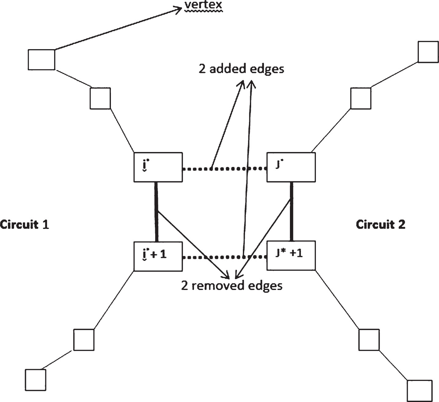
A Hamiltonian circuit.

where i = 1, 2, …, |V (C₁) | and j = 1, 2, …, |V (C₂) |

If a few pairs of edges satisfy this condition, we select a pair of the edges arbitrarily.

After that, we remove edge e (i * , j * +1) ∈ E (C₁) and edge e (i * , j * +1) ∈ E (C₂) and next we add the following two edges: e (i * , j *), e (i * +1, j * +1) – see Fig. 1. We go to step 3.

By this way we construct a Hamiltonian circuit $C_{H}^{h}$ and count $w [C_{H}^{h}]$ .

To present how this algorithm “works”, let us consider a complete weighted graph K₆ as an example (Fig. 2).

Fig.2

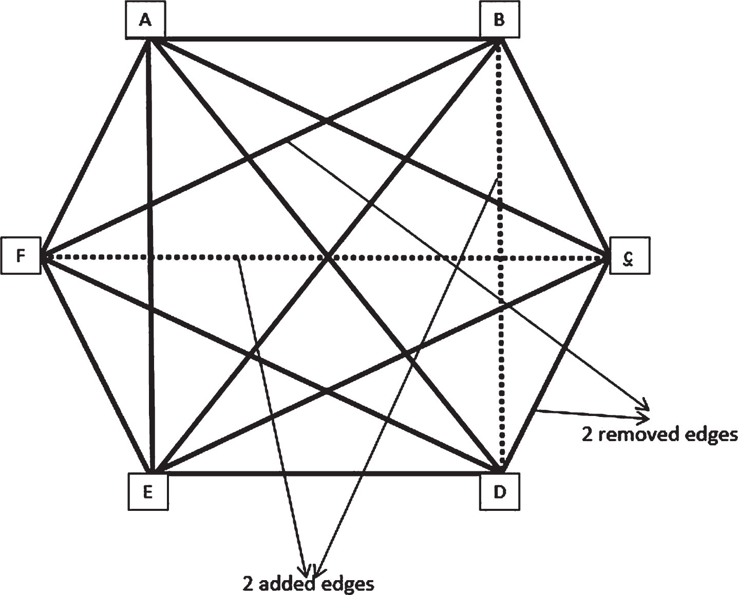
Graph K₆.

In our example K₆ we have |V| = n = 6, |E| = 15 and | { CH } | = (n - 1) !/2 = 60. The 15 edges have the following weights assigned to them:

w[e(F,A)] = 1

w[e(F,B)] = 5

w[e(F,C)] = 5

w[e(F,D)] = 12

w[e(F,E)] = 14

w[e(A,B)] = 9

w[e(A,C)] = 12

w[e(A,D)] = 12

w[e(A, E)] = 11

w[e(B,E)] = 6

w[e(B,D)] = 7

w[e(B,C)] = 13

w[e(C,D)] = 2

w[e(C,E)] = 3

w[e(D,E)] = 2

According to step 1 we obtain an ordered set <L₁>:

<L₁> = < w [e (F, A)] = 1 < w [e (C, D)] = w [e (D, E)] = 2 < w [e (C, E)] = 3 < w [e (F, B)] = w [e (F, C)] = 5 < w [e (B, E)] = 6 < w [e (B, D)] = 7 < w [e (A, B)] = 9 < w [e (A, E)] = 11 < w [e (F, D)] = w [e (A, C)] = w [e (A, D)] = 12 < w [e (B, c)] = 13 < w [e (F, E)] = 14 >

The six first edges in this ordered set are marked in the sequence above by bold font. Because condition in step 3 is not satisfied we go to step 4 and define set T ={ A, B }.

In the next step we identify and remove from set E (L₁) edge e_max = e (F, C) = 5, set T is not changed. In step 6 we define edge e₁ = e (A, B) and update graph $L_{i}^{*}$ = $L_{i}^{*}$ ∪ e (A, B). We go to step 2 and obtain set <e (F, A), e (A, B), e (F, B), e (E, C), e (C, D), e (D, E) >.

It is easy see that the edges from the set {e (F, A), e (A, B), e (F, B), e (E, C), e (C, D), e (D, E)} can create 2 cycles C₁ = {F, A, B, F} and C₂ = {E, C, D, C}. We observe that these two cycles cover all vertices of the graph K₆. We go to step 7. In this step we link two cycles C₁ and C₂ under condition (*) from the algorithm. We notice that:

min {w [e (A, E)] + w [e (B, D)], w [e (A, D)] + w [e (F, E)], w [e (A, C)] + w [e (B, D)], w [e (B, C)] + w [e (A, D)], w [e (B, E)] + w [e (F, D)], w [e (F, D)] + w [e (A, C)], w [e (F, C)] + w [e (B, D)]} = w [e (F, C)] + w [e (B, D)] = 7 + 5 = 12.

As we see, we add 2 edges: e(F,C), e(B,D), which connect cycle C1=F, A, B, F and cycle C2=E, C, D, C and we remove 2 edges: e(F,B) and e(D,C).

As a consequence we obtain a Hamiltonian circuit $C_{H}^{h} = {{A, F, C, E, D, B, A}}$ , where $W [{C_{H}^{h}}] = 27$ . The obtained solution constructed by our heuristic procedure is of course an approximation of the optimum. In our example of the graph K₆, optimum constitutes the following Hamiltonian circuit $C_{H}^{opt} = {{F, C, D, E, B, A, F}}$ where weight $W [{C_{H}^{opt}}] = 25$ . This is only one Hamiltonian circuit in our example with such optimal weight.

We can observe that there is little difference between our approximation solution and optimum.

3 Properties of the algorithm

Now we will prove the correctness of the algorithm.

Theorem 1. Steps 1–7 of the algorithm give some approximate solution of the STSP in a finite number of steps.

Proof. We can observe below the following facts.

In any graph K_n, n selected edges cause that each vertex v ∈ V (K_n) is incident to some edge e ∈ E (K_n) and there are two vertices v₁ and v₂ which satisfy deg(v_i) ≥ 2, i = 1, 2. There are no isolated vertices.

Steps 5, 6 always define two edges e_max and e_l – these rules decide about finiteness of our algorithm.

It’s obviously that |L_i| = n for each iteration i.

Furthermore, if for each vertex v ∈ V (K_n) deg(v) = 2 and condition in step 3 is satisfied, we obtain a Hamiltonian circuit or in other case we have set {C_A}.

Step 6 decreases the cardinality of set T at least by one.

For any graph G (V, E), if for each vertex v we have deg(v) ≥ 2, then |E| ≥ n.

For any graph G (V, E) we have ∑_v∈V deg(v) = 2|E| – elementary fact from the graph theory.

It is obvious that step 7 of the algorithm decreases the number of simple circuits at least by one.

We conclude that:

it is an obvious fact,

follows from (2),

it is an obvious implication,

follows from the property of construction of step 6 in the algorithm,

follows from (7), because of the fact that in the borderline case of graph $L_{i}^{*}$ .i.e. for n vertices with deg(v) = 2 we have

| E | \geq \frac{2 * n}{2} = n

Fact (2) follows because of the following:

e_max is always defined – we conclude this from fact (1) and step 5,

if in some iteration i the edge e_l cannot be defined, then we have n –1 edges, |T| = 1 and ∀_v∈V∖T deg(v) ≥ 2. Then from one side we have

$\sum_{v \in V (L_{i}^{*})} deg (v) \geq 2 (n - 2) + 2 * 3 = 2 n + 2$

This is borderline case with n - 2 vertices, where have deg(v) = 2 and 2 vertices with deg(v) = 3. From other side we have (n - 1) + 1 = n edges because of one vertex belonging to T (step 4 of the algorithm). We obtained a contradiction.

Based on (3-6) and (8) we conclude thesis of our theorem (q.e.d).

Let’s consider the problem of computational complexity of the algorithm. In our case we assume the parameter m as a characteristic of the dimension in our problem, where m is the number of edges in a complete graph K_n. Considering the seven consecutive steps, we conclude that:

step 1 costs at most O(m*log(m)) elementary operations,

step 2 costs at most O(m) elementary operations,

step 3 costs at most O(m) elementary operations,

step 4 costs at most O(m) elementary operations,

step 5 costs at most O(m) elementary operations,

step 6 costs at most O(m) elementary operations,

step 7 costs at most O(m²) elementary operations.

Hence we obtain the following theorem.

Theorem 2. The described algorithm required at most O (m²) elementary operations, where m is the number of edges.

Proof. The proof we obtain from two facts:

the properties of the given algorithm,

if the algorithm works on the data of size m (m – natural number) at the time c*m² for arbitrary constant c, then we say that the computational complexity is O (m²) [11]. In our case c = 7 (seven steps of the algorithm).

4 An estimation of the bound

We are interesting in the estimation of the bound for our heuristics. We can show that if the following inequality $W [e_{l}^{C_{A}}] \leq 2 w [e_{k}^{opt}] (* *)$ is satisfied for any fixed vertex v^* ∈ K_n, where $w [e_{k}^{opt}] = max {w [e_{k^{'}}^{opt}], w [e_{k^{″}}^{opt}]}$ and any edge $e_{l}^{C_{A}} or e_{k}^{opt}$ is incidental to this vertex, then we obtain.

Theorem 3. The algorithm gives the following ratio: $\frac{w [C_{H}^{h}]}{w [C_{H}^{opt}]} 3$

Proof. Let’s consider any vertex v * ∈ Kn. We have three options:

Two edges incident to this vertex belong to some cycle C_A, but not to $C_{H}^{opt}$ ,

Only one edge $e_{l}^{C_{A}}$ covers with edge that belongs to $C_{H}^{opt}$ ,

Both edges $e_{l}^{C_{A}}$ belong to $C_{H}^{opt}$ ,

We are interested in the first two cases. Assume that inequality (**) is satisfied for these two cases. Let s be such a number of the edges $e_{l}^{C_{A}}$ that satisfy (**), We denote them by ${e_{k}^{opt}}_{i = 1}^{s} \subset E (C_{H}^{opt})$ .

Surely, if we have under taking the inequality $w [e_{k}^{C_{A}}] \leq 2 w [e_{k}^{opt}]$ then the following estimation is satisfied; $\begin{matrix} w [{C_{A}}] \leq w [C_{H}^{opt}] + \sum_{k = 1}^{s} (w [e_{k}^{C_{A}}] - w [e_{k}^{opt}]) \\ \leq w [C_{H}^{opt}] + \sum_{k = 1}^{s} (w [e_{k}^{opt}]) . \end{matrix}$ (7)

It is clear that for any two edges $e_{k}^{opt}, e_{l}^{opt}$ that belong to $C_{H}^{opt}$ and simultaneously link two simple cycles $C_{A}^{i}$ and $C_{A}^{j}$ condition (*) is satisfied by step 7 of our algorithm. Therefore for k-1 connections of simple disjoint cycles that define C_A (our heuristics) and when we introduce index we have: $\sum_{i = 1}^{k - 1} min_{i} \leq \sum_{i = 1}^{i = 2 (k - 1)} w [e_{i}^{opt}] .$ (8)

In inequality (8) “min_i” denotes some constant.

Using (7), (8) and the properties of the algorithm, we obtain: $\begin{matrix} w [C_{H}^{h}] \leq w [{C_{A}}] + {the sum of the 2 (k - 1) \\ edges that link k cycles of any set {C_{A}} = w [{C_{A}}]} \\ + \sum_{i = 1}^{k - 1} min_{i} \leq w [C_{H}^{opt}] + \sum_{k = 1}^{s} w [e_{k}^{opt}] + \sum_{i = 1}^{i = 2 (k - 1)} \\ w [e_{i}^{opt}], where s < n and 2 (k - 1) < n \end{matrix}$ (9)

Dividing both sides of inequality (3) by $w [C_{H}^{opt}]$ we have: $\frac{w [C_{H}^{h}]}{w [C_{H}^{opt}]} = 1 + q_{1} + q_{2} < 1 + 1 + 1 = 3,$

because of {q₁, q₂ } ∈ (0, 1). This ends proof of the theorem (q.e.d.).

5 Conclusions

In this paper we analyzed symmetric classical travelling salesman problem (STSP) without using triangle inequality. We presented some heuristics, where under some condition the ratio $\frac{w [C_{H}^{h}]}{w [C_{H}^{opt}]} < 3$ can be obtained with O (m²) computation complexity, where m is the number of edges in the complete graph K_n.

In [4] Christofides showed heuristics that require O (n³) computations for matrices satisfying the triangle inequality. Some modifications of this heuristics are contained in paper [5], with polynomial complexity.

Sahni and Gonzales in their article [1] proved, that if the triangle inequality does not hold then, for constant c ≥ 1 the problem of finding an approximate tour $C_{H}^{h}$ such that $w [C_{H}^{h}] \leq c * w [C_{H}^{opt}]$ , is NP-complete.

The survey of the latest results of experimental calculations can be found in paper [10]. This survey is limited to selected approaches, because it is not possible to cover all off them. The authors of this paper discussed only the most relevant approaches such as:

Brute Force Method,

Greedy Approach,

Nearest Neighbour Heuristic,

Branch and Bound Method,

2-opt Algorithm,

Greedy 2-opt Algorithm,

Genetic Algorithm,

Neural Network,

Simulated Annealing.

The efficiency of these heuristics are given as a relation between number of cities and time in sec to find heuristic a solution. In some papers in the literature the efficiency of the discussed heuristics is given in the form of the graphs of a function as the relation between two parameters - time and cities. There are of course possible combinations of well known algorithms, for example a combination of the Nearest Neighbour and Minimum Spanning Tree algorithms [9].

Our result is rather theoretical nature, without experimental calculations. In some way our algorithm presented in this paper can be treated as a compilation of the Nearest Neighbour Heuristic and Greedy Approach. A reader interested in the history of the TSP and some implementations can find specific information in paper [7] and [8].

References

Sahni

and Gonzales

, P-complete approximation problems, Journal of the ACM 23 (1976), 555–565.

Papadimitriou

C.H.

, Computational complexity, Addison-Wesley Publishing Company, Inc, 1994.

Kuhn

H.W.

, The Hungarian method for the the assignment problem, Nav Res Log Quart 2(1-2) (1955).

Christofides

, Worst-case analysis of a new heuristics for the travelling salesman problem, GSIA, Carnegie-Mellon Univ., 1976.

Cornuejols

and Nemhauser

G.L.

, Tight bounds for Christofides travelling salesman heuristics, Working paper No. 7627 Center for Operations Research and Economics, Universite Catholique de Louvain (Louvain-la-Neuve), 1976.

Basirzadeh

, Ones assignment method for solving travelling salesman problem, Journal of Mathematics and Computer Science (JMSC) 10 (2014), 258–265, Shahid Chamran University, Ahvaz, Iran.

Cook

, History of the TSP The travelling salesman problem, Georgia Tech, 2009.

Maredia

, History, analysis and implementation of travelling salesman problem (TSP) and related problems, Department of Computer and Mathematical Sciences, University of Houston-Downtown, 2010.

Fatma

, Karkory

and Abudamola

, Implementation of heuristics for travelling salesman problem using nearest neighbour and minimum spanning tree algorithms, International Journal of Mathematical, Computational, Natural and Physical Engineering 7(10) (2013).

10.

Abid

M.M.

and Iqbal

, Heuristic approach to solve traveling salesman problem, TELEKOMNIKA, Indonesian Journal of Electrical Engineering 15(2) (2015), 300–396.

11.

Aho

A.V.

, Hopcroft

J.E.

and Ullman

J.D.

, The design and analysis of computer algorithms, Addison-Wesley Publishing Company, 1974.