Training contextual neural networks with rectifier activation functions: Role and adoption of sorting methods

Abstract

Contextual neural networks are effective and very usable machine learning models being generalization of multilayer perceptron. They allow to solve classification problems with high accuracy while strongly limiting activity of connections between hidden neurons. Within this article we present novel study of properties of contextual neuronal networks with Hard and Exponential Rectifier activation functions and of their influence on behavior of the Generalized Error Backpropagation method. It is used to show how to optimize efficiency of the sorting phase of this algorithm when applied to train evaluated models. This considerably extends our previous related paper which was limited to analysis of contextual neuronal networks with Leaky Rectifier and Sigmoidal activation functions. This article includes wide description of contextual neural networks and generalized error backpropagation algorithm as well as the discussion of their connection with self-consistency paradigm, which is frequently used in quantum physics. Also the relation of the latter with sorting methods and considered rectifier functions during training of contextual neural networks is studied in details. Conclusions are backed up by the results of performed experiments. Reported outcomes of simulations confirm the ability of contextual neural networks to limit activity of connections between their neurons and – what is more important – indicate the detailed rules of selection of the most efficient sorting algorithm for updating scan-paths of contextual neurons that are using Hard and Exponential Rectifier activation functions. Presented results have considerable value both for research and practical applications – especially where the efficiency of training of contextual neural networks is crucial.

Keywords

Classifiers self-consistency aggregation functions scan-paths

1 Introduction

Contextual neural networks (CxNNs) are generalized versions of existing neuronal models. Transfer functions of their hidden nodes aggregate signals conditionally and in multiple steps [1]. Such solutions can be applied successfully to analyze data sets from benchmarks repositories and to classify data observed in practice [2, 3]. It was presented that they can increase accuracy of fingerprint analysis for crime investigations [4, 5]. One can also find their usefulness in cognitive radio while predicting communication channels availability and in research no how computationally aware are machine learning algorithms [6].

Neuronal models with context-dependent aggregation schemes can achieve higher levels of generalization than their counterparts including MLP [3]. They also give possibility of high reduction of activities of neurons’ inputs while not limiting precision of the value of neurons’ output. And what is important – this property manifests itself not only when the model is being trained but also afterwards. In the effect it may limit energy and time related cost of application of CxNNs under high constraints (e.g. in IoT embedded systems or android robots). Controlling for which input data the connection between neurons should be active is an adaptive process. Thus given contextual neuron can activate various sets of its’ inputs for non-identical input vectors. It is also not reading and not analyzing data from input connections which are not useful to compute its’ output for current inputs vector. And in the effect contextual NN can be perceived as a grey instead of a black box system. The analysis of how active are neurons’ dendrites of the input layer of CxNN may reveal if given attribute and its’ values are crucial for calculation of the model outputs in case of given data vectors. Thus knowing the average activity of CxNN’ inputs allows to show relative importance of each data attribute as perceived by the trained model.

In detail, contextual neurons are aggregating input values in many instead of single step. Different subsets of input signals are aggregated in subsequent steps and between them the actual accumulated activation value is used to check if neurons’ output can be accurately calculated. It is assumed that groups of more important inputs are processed before those which are less important. Which input belongs to which aggregation group is set adequately for each hidden node by the training algorithm. In reference to the research on saccadic eyes movements and scan-paths lead by Stark, a list of aggregation groups is named a “scan-path” [7]. It is related to the fact that considered aggregation functions are processing subgroups of input signals in many steps and conditionally – till accumulated value of partial activations is not higher than assumed fixed value. Sigma-if and PRDFA are the two example cases of multiple possible aggregation functions [1].

What is interesting, in comparison with non-contextual neurons only two extra real-valued parameters need to be considered to express more complicated behaviour of neurons which are aggregating signals conditionally. Those are two constants which can be common for all hidden neurons: number of groups and aggregation threshold. Moreover, their values may be chosen before training of CxNN based on results of earlier analyses of such models for many classification problems [2]. Those two additional parameters are enough to construct methods of conditional signals aggregation which encode scan-path related groupings of inputs within already existing weights of edges between nodes of neuronal network. But usage of such construction forces training of CxNN models with special methods such as generalized back-propagation algorithm (GBP) based on the self-consistency paradigm [8 –10]. It allows to optimize non-continuous and non-differentiable scan-paths with gradient method by optimization of related continuous and differentiable weights of connections. It improves functionality and ease of creation of CxNNs in relation with other models with contextual neurons such as Sigma-Pi, Clusteron [11] and Spratling-Hayes [12].

In contrast to the classical backpropagation algorithm which by definition is not performing sorting [2], GBP method uses sorting to implement the self-consistency method [1 –3, 9]. What is important, improper selection of the sorting algorithm can drastically decrease time efficiency of the GBP training process. To overcome this problem, in this article we show how to select and tune sorting algorithms for use within GBP when trained neuronal networks are using nodes with Hard and Exponential Rectifier activation functions [13, 14]. This extends earlier results presented in our conference paper [15], which were limited to contextual models with Sigmoidal and Leaky Rectifier activations. Hard and Exponential Rectifier activation functions are frequently used in deep learning applications. Thus exposing their relation with GBP and sorting methods seems to be of considerable importance both for research and practical applications of contextual neural networks.

Further parts of the article are constructed as follows. Section 2 briefly describes the GBP method. Next in Section 3 details of sorting phase of GBP algorithm and discussion of its’ eventual improvement are presented. On this basis in Section 4 we present results of experiments that show which sorting methods allow the highest time performance of self-consistency within GBP for neural networks with Hard and Exponential Rectifier activation functions. Finally Section 5 includes discussion if presented measurements may allow to identify earlier not analyzed properties of CxNNs and GBP method, in particular the effect of self-consistency on the content of scan-paths of neurons.

2 Generalized error backpropagation algorithm

The Generalized Error Backpropagation method was created as an extended version of well known BP algorithm. It was created to construct artificial neuronal models that make use of functions such as Sigma-if that can aggregate input signals conditionally and in many steps [1, 2]. Considered GBP algorithm combines gradient-based search with self-consistency method widely used in quantum physics [8 –10]. This allows to optimalize together weights of connections and discrete, non-differentiable indexes of connections grouped within neuronal scan-paths.

Maintaining reciprocal relationship between the two mentioned sets of factors is the key to abilities of the GBP algorithm needed to train CxNNs. This dependency is created by making the assumption that non-continuous factors can be functions of weights. This relation, further denoted as Ω, includes two phases. First: sorting neuron’ dendrites by values of their weights and, in the second step: partitioning sorted list of dendrites to K clusters of the same size. In the effect of such procedure N/K dendrites having the top values of weight are assigned to the first most important cluster of the scan-path, following N/K dendrites having the top values of weight are assigned to the next cluster, etc. This forms the basis for execution of multi-step aggregation functions, in which clusters of input signals are loaded and aggregated one by one until used stopping clause is not fulfilled. The general block diagram of the GBP algorithm is presented on the Fig. 1.

Fig.1

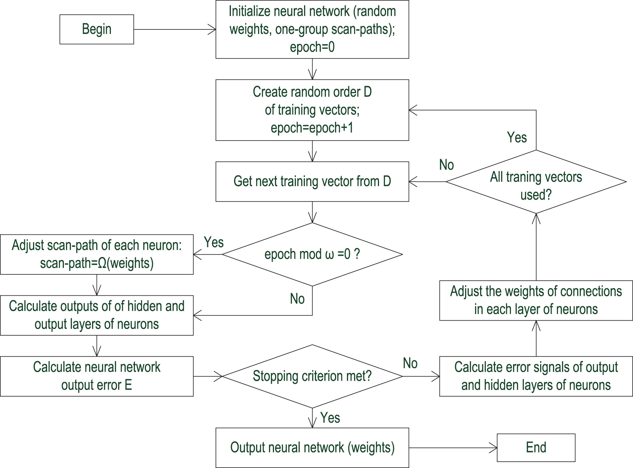
Block diagram of the generalized error backpropagation algorithm with scan-path creation function Ω and scan-paths update interval ω.

While looking at this flowchart it is worth to analyze how the self-consistency bound betwixt parameters of neuronal aggregating function and connection weights is controlled by the interval ω. At the beginning of CxNN training with GBP all inputs of hidden nodes are included in the initial, most important clusters of related scan-paths. It is done to not exclude any dendrites from aggregation at the beginning of the training. Next, after every ω epochs function Ω updates scan-path of each neuron depending on the current values of weights of dendrites.

In the effect, the value of interval ω may have considerable impact on the training. When ω =∞ (or the assumed count of clusters K is one) the work of GBP method is identical as of the standard BP algorithm. In such case CxNN making use of hidden nodes with multiple-step aggregation acts as the MLP.

Contrary, when ω is close to one and assumed number of groups K is greater than one the updating scan-path of each neuron after every ω epochs periodically reorganizes the error space of the neural network. In general the evolution of the error space can distract the training process. But experiments show for K > 1 and 5< ω << ∞ that the update of the scan-path increases the error of the neuronal model only temporarily. During next few epochs the GBP adapts the model to the new error space and the level of output error can be decreased afresh, frequently bringing also limitation of the activity of links between neurons.

In the effect of the above, CxNN models constructed by the GBP method can have higher level of generalization and lower average activity of connections than their non-contextual versions built by the BP. The source of this fact is that periodic updates of the scan-paths together with conditional character of multiple-step aggregating functions of neurons, create solution similar to the dropout regularization method frequently applied in deep learning. However, from two other perspectives both methods are fundamentally different. The signals analyzed by the neural network have no influence on the dropout, while the decision space of each contextual neuron is adapted to actual input vector considering all knowledge gathered by the neural network during its’ training with the GBP. Additionally, dropout limits the average activity of inputs of hidden neurons exclusively while the training process, and CxNNs can decrease it also when the GBP is over. Thus aggregating methods of CxNNs can be perceived as useful tools both for simple neuronal networks and in the case of bigger structures with convolution layers.

The above presentation of the GBP method suggests that sorting of dendrites by their weights can be the source of considerable computational cost. This can be especially important for hidden neurons with high counts of inputs. Thus it can be valuable to further describe and analyze details of usage of sorting methods by the GPB algorithm.

3 Reordering dendrites in scan-paths by GBP

The crucial aspect of the generalized error backpropagation method, as signaled in the preceding section, is the procedure of updating a neuron’s scan-path, carried out as the sorting of the inputs. The gradient searching, performed by the GBP, is in this way merged with the idea of self-consistency. However, the non-triviality of the problem of assigning the right sorting method for the needs of the GBP approach is not difficult to observe. It arises from the fact that the performance of each round of inputs sorting can be influenced by at least two factors. One of them would be a given hidden neuron’s count of dendrites since the performance of a sorting algorithm in question can be significantly influenced by the number of elements to be ordered. The other factor is constituted by the data content. But in general, it is not easy to predict changes of scan-paths for given training data. This is because subsequent scan-path updates can change the weights of connections slightly, even hardly at all, or significantly – in the effect of the GBP’s parameter values and the information within training data. Finally, the behavior of various sorting methods can vary according to whether the data is partially or fully sorted. As a result, their computational performances may deviate significantly in both directions from their mean values.

In order to analyze how a sorting algorithm influences the performance of the generalized error backpropagation, let us first inspect the way in which the training method utilizes a sorting scheme. In the first steps of training, the input connection weights get assigned random values. Simultaneously, all the inputs get allocated to the first aggregation cluster in order to guarantee they will be active within the initial rounds of training. Thus initial ω training epochs can end in such a way that the weights W of neuron inputs of given indices I and their assignments to the scan-path clusters G have the following example values:

W = [0.4, 0.2, 1.2, 0.7, 0.4, 0.9, 1.1] //connect. weights

I = [1, 2, 3, 4, 5, 6, 7] //indices of inputs

G = [1, 1, 1, 1, 1, 1, 1] //clustering

Next, neuron input connections are sorted by their weights and split to assumed count of clusters K. All clusters will include an equal count of inputs whenever applicable. If the number of neuron inputs N is undividable to K equally sized clusters, the remaining set of inputs falls into the last cluster. Later, in the course of the next epoch, the signals coming from the inputs categorized as group one will be aggregated first. Next, as stated by the aggregation function’s details, input values from the remaining groups will be aggregated conditionally. An example of a sorted connection weight vector W with an assignment to the groups in the vector G isgiven below:

W = [1.2, 1.1, 0.9, 0.7, 0.4, 0.4, 0.2 //connect. weights

I = [3, 7, 6, 4, 5, 1, 2] //indices of inputs

G = [1, 1, 2, 2, 3, 3, 3] //clustering

This kind of weights ordering method and process of reallocating inputs of neuron to respective aggregation clusters is carried out after every ω training epochs. It allows to maintain partial mutual dependence of the inputs clustering and the modified values of weights, as expected by the self-consistency mechanism.

A crucial fact to notice is that when the same data are provided to each sorting method, they generate identically sorted lists of values. Thus for every sorting procedure the GBP will produce the same resulting neural network for identical values of input parameters. But the training efficiency of various sorting approaches will vary both on the count of inputs of the network’ nodes (relates to the average computational complexity of sorting for random data) and on the data to be sorted (relates to the computational complexity of sorting for data of particularorder).

Thus one can observe that the mean efficiency of sorting may be related to the systematic manner the GBP algorithm modifies weights of connections and their assignment to aggregation clusters. When weight values differ only by a small amount in consecutive epochs, for related neuron the second sorting processes with an almost sorted elements. In these cases, the topmost efficiency can be displayed by approaches designed and optimized for ordered data, e.g. the Insertion-sort method. The circumstances will, however, be different when the weights between epochs get modified so largely that the original assignments of connections to aggregation clusters will be affected noticeably as well. Then, for any given neuron, the sorting method will need to process considerably unordered elements. Such cases are handled more effectively by approaches such as the Quick-sort. And it is hard to predict for which data vectors the activity of connections, changes of weights and related scan-paths will be high for given activation functions such as e.g. Hard and Exponential rectifier. Thus the relation between using those activation functions and proper selection of sorting method for GBP needs to be found experimentally.

From this standpoint, this article deals with experimental verification of various sorting algorithms’ efficiency for those situations when contextual neural networks are trained via the GBP algorithm. It may appear valuable in prescribing according to what rules a sorting algorithm should be adopted for a particular contextual neural network. And its’ even greater importance lies in the fact that it will enable the analysis of the GBP approach in terms of interdependencies between the scale of weight modifications in consecutive sortings and the prioritization of hidden neuron input aggregation. The neuron inputs’ aggregation priorities as well the correlated NN error space may happen to be altered immensely following each weight-sorting round. Then the training could be perceived more like random process. It can also turn out that the initial aggregation priorities are not changed by the sorting. It can indicate towards the self-consistency paradigm as being irrelevant with respect to the training results. Does it mean training via the GBP learning rule is governed by some, above-mentioned phenomenon? Is it determined by how frequently the scan-paths get updated in CxNNs with broadly used rectifier activation functions? Finding answers to these questions would result in a broad expansion of how deeply and completely we understand the GBP algorithm’s properties.

4 Results of experiments

For the purpose of finding an answer to the question posed in the preceding section, we have performed experiments in which CxNNs with Hard and Exponential Rectifier activation functions have been trained via the GBP algorithm, using six variants of sorting methods. We have used the Insertion-sort, recursive Quick- and Merge-sort, the Bubble-sort, the Optimized-, and Two-Way Optimized Bubble-sort (abbreviated as ISort, QSort, MSort, BSort, OBSort, and TWBSort, respectively) [16 –18]. The QSort, MSort and ISort were unmodified and unimproved, i.e. in their generic implementations. For example, the middle element was used as a pivot by the QSort, and short subpartitions were sorted by means of no particular technique [17]. The ISort did multiple switch operations instead moving larger prior to the inserted values, and did not initially placed the smallest element at the beginning [16]. Sorting methods without the mentioned and related improvements were used since such modifications are usually introduced to speed-up processing of sets of random values. We anticipate that such an assumption may happen to be invalid for the GBP algorithm, in which case the data can be often partly sorted. In the effect, basic versions of sorting methods are expected to make the results easier to understand and interpret. It can also stimulate finding such optimizations that would be particularly suitable for the GBP method.

It is worth to notice that the time effectiveness of sorting methods used within GBP is related to the length of scan-path of the neuron and not to the number of processed training vectors. And initial experiments have shown that measurements for scan-paths of length up to 60 are enough to formulate the rules of selecting and tuning sorting methods for use with GBP algorithm. But we keep the analyzed range of scan-path length from 4 to 244 to allow easy comparison of presented results with outcomes of our earlier studies [15]. We also select data sets that include more than 100 vectors what is enough to achieve the average relative error of measurements for single sorting to be below 1%. Thus in our experiments, UCI Machine Learning Repository problems, such as Soybeans, Wines, Hypothyroid, Lung Cancer, Iris and Sonar, were used to train contextual neural networks via the GBP algorithm.

Across the entire network, every neuron used the Hard Rectifier or Exponential Rectifier functions for activation and Sigma-if function for aggregation. [2 , 14]. On the basis of the aggregation threshold φ * =0.6, the aggregation functions performed a split of the inputs of all the hidden neurons into K groups. A single binary input for each value stood for nominal attributes, and continuous attributes were normalized to span the range of <0, 1> (one-hot encoding). Basing on prior experimental results, the number of hidden-layer neurons and groups K were determined in such a way, so that obtained models displayed a significantly declined inter-neuron connection activity as well as near-optimal classification accuracies. Table 1 shows the resultant NN architectures that were put to use in the experiments.

Table 1
Details of contextual neural network architectures applied against chosen UCI ML Repository benchmarks

Data set Count of data attributes Count of inputs of neural network Count of hidden neurons (N) Count of outputs (data classes) Total count of hidden connections Count of neuron aggregation clusters (K)

Iris 4 4 10 3 70 3

Wines 13 13 10 3 160 3

Hypothyroid 29 35 10 5 400 14

Sonar 60 60 10 2 620 10

Soybeans 35 134 20 19 3060 22

Lung Cancer 56 244 3 3 741 3

Data set	Count of data attributes	Count of inputs of neural network	Count of hidden neurons (N)	Count of outputs (data classes)	Total count of hidden connections	Count of neuron aggregation clusters (K)
Iris	4	4	10	3	70	3
Wines	13	13	10	3	160	3
Hypothyroid	29	35	10	5	400	14
Sonar	60	60	10	2	620	10
Soybeans	35	134	20	19	3060	22
Lung Cancer	56	244	3	3	741	3

The GBP parameters took the following values: training step α = 0.01, the interval of updating aggregation clusters ω = 25, the stopping criterion: the training data perfectly classified or a constant (not growing) classification accuracy for at least 300 consecutive epochs of training. Momentum and annealing of training steps were not applied.

Experiments were carried out in a software developed with Delphi 7 environment; the standard included linear congruential pseudorandom generator was applied to provide GBP with random values. The seed took the following values for each set of values of the above parameters: 0, 2013420422, 350932796, 429462840, 723512745, 127401735, 323664106, 634385610, 345071639, 519168307. Repeating each training of the CxNN 10 times for a given set of parameters was meant to verify the identicalness of the obtained models as well as an increase in the precision of the measurement of the training’s cost. Since an assessment of classification properties of CxNNs based on the GBP was not the goal of the analyzes under discussion, a cross-validation was not applied. Therefore, for a given benchmark, all training vectors were used in eachtraining.

The measures determined during each simulation were as follows:

a sorting algorithm’s computation cost,

the average CxNN classification error,

the minimum, mean and maximum activities of the neural network’s internal connections,

the count of training epochs.

The network of the maximum mean classification accuracy noted when running the GBP had its hidden connections’ activity logged. Each individual sorting’ amount of computations was quantified by means of the 64 bit TS Counter register integrated within the main CPU. By totaling the processor’s clock ticks the cumulated execution cost of a given sorting algorithm is calculated during a given training session. Next, a single sorting round’s mean cost was calculated as the ratio between the total sorting time and the count of the sorting algorithm invocations. The simulation program was executed in highest-priority mode to limit the operating system’s impact on the precision of the measurements.

Table 2 presents the results of the experiments. It includes the average values of classification errors, connections’ activity of CxNNs as well as the number of epochs of their training. The GBP stopping criterion was defined as follows: a perfect classification or a stable, non-decreasing classification error during the 300 most recent epochs.

Table 2

The mean classification-errors (cerr), training epochs (trep) as well as minimum, mean and maximum activities of hidden neurons’ connections (hca) in Contextual Neural Networks processing exemplary UCI benchmarking data sets. In use were neurons with Sigma-if aggregation and Hard- (HR) or Exponential Rectifier (ER) activation functions

Benchmark problem	Act.funct.	Cerr [% ]	Trep [1]	Mean hca [% ]	Max hca [% ]	Min hca [% ]
Iris	HR	2.7±0.9	630±72	93.7±1.2	100±0	84.6±3.6
Wines	HR	0±0	32±9	94.3±4.0	100±0	86.8±9.3
Hypothyroid	HR	4.7±0.5	411±87	74.8±3.9	91.3±1.7	55.0±5.4
Sonar	HR	0±0	126±34	75.8±2.7	92.6±2.1	52.2±4.7
Soybeans	HR	2.5±4.3	958±223	86.0±5.0	100±0	57.4±7.2
Lung Cancer	HR	0±0	78±90	78.9±8.2	91.1±4.4	64.5±13.2
Iris	ER	6.6±2.1	650±176	94.4±1.4	100±0	81.1±5.5
Wines	ER	0.2±0.3	206±133	96.4±2.4	100±0	82.1±11.5
Hypothyroid	ER	6.0±0.1	632±204	91.5±4.2	98.5±2.6	59.3±4.2
Sonar	ER	3.3±2.5	740±209	76.8±9.4	98.6±2.3	50.0±8.9
Soybeans	ER	27.0±1.1	504±180	93.5±2.0	100±0	66.2±6.1
Lung Cancer	ER	0±0	56±12	80.7±6.1	93.1±6.1	64.7±8.1

Within the obtained results, one can observe that connections activities are considerably decreased. It can be also seen that CxNNs of larger structures (for the Sonar, Hypothyroid, Soybeans and Lung Cancer data sets) are able to present decreased activity levels of connections, compared to more limited architectures (here for the Wines and Iris). The two phenomena were anticipated as they had been known from prior experiments [3]. But what is important, their existence shows a contextual nature of the neuronal models created via the GBP. As a result, analyzed simulations can constitute a foundation from which other probable relations between the properties of CxNNs training via the GBP and the computational efficiency of considered sorting methods could perhaps be recognized and derived.

Table 3 summarizes the observed average relative computational cost across 6 analyzed algorithms when applied for updating neurons’ scan-path by means of the GBP algorithm. The measurements were performed by re-running the GBP for each sorting method against the same NN architectures, the benchmark problem set as well as other linked attributes (e.g. the initial values of connection weights, the pseudo-random generator seed, etc.). As far as each of the sorting methods is concerned, the result of training a model was the very same for identical values of GBP parameters. This is caused by the fact that an identical outcome is returned for identical input data by all evaluated sorting algorithms. Thus, the result of the GBP cannot be modified by switching between sorting methods. However, the sorting algorithms may vary with respect to the total count of operations required to completely sort given data. In the result, we can observe different costs of using analyzed sorting algorithms within the GBP. To make the results easier to analyze, every achieved computational cost is expressed as a percentage fraction of the ISort’s measured cost. Accordingly, Table 3 contains also the hidden neurons’ scan-path length. We understand the scan-path length as the total count of values that the GBP algorithm needs to sort during a given neuron’s single scan-path update.

Table 3

The mean relative cost of scan-paths sorting per neuron per epoch done while training of CxNN via the GBP for selected UCI data sets, sorting methods and two neuronal activation functions: Hard Rectifier (HR) and the Exponential Rectifier (ER)

Benchmark problem	Act. funct.	SPL [1]	MSort [% ]	QSort [% ]	ISort [% ]	TWBSort [% ]	OBSort [% ]	BSort [% ]
Iris	HR	4	134.0±4.5	115.3±3.3	100	104.2±3.9	114.2±11.5	105.3±3.1
Wines	HR	13	170.4±22.8	126.2±7.9	100	151.7±8.9	156.3±10.5	159.6±10.0
Hypothyroid	HR	35	110.1±6.9	89.8±6.9	100	212.6±13.5	230.5±11.8	235.2±15.1
Sonar	HR	60	82.8±1.3	69.0±1.6	100	238.5±2.2	269.2±4.0	265.7±2.7
Soybeans	HR	134	48.4±0.9	41.6±1.2	100	261.8±0.5	304.8±1.7	293.8±5.6
Lung Cancer	HR	244	32.7±0.4	27.8±0.6	100	269.2±1.4	317.3±1.7	300.6±3.6
Iris	ER	4	139.6±20.8	122.1±8.0	100	102.6±7.1	107.8±7.1	104.5±6.7
Wines	ER	13	156.7±6.9	123.8±5.7	100	145.2±2.8	158.2±8.0	156.2±4.5
Hypothyroid	ER	35	120.1±11.3	88.0±7.2	100	241.0±31.4	197.4±25.7	231.8±18.3
Sonar	ER	60	82.8±1.7	68.6±1.7	100	239.0±1.4	269.9±1.3	266.0±1.4
Soybeans	ER	134	45.0±0.6	38.3±0.7	100	262.5±3.9	301.3±4.1	291.6±4.4
Lung Cancer	ER	244	32.9±0.5	27.8±0.7	100	270.0±0.8	317.8±1.6	304.0±1.6

Aggregation function: Sigma-if. The scan-path length (spl) is the count of a hidden neuron’s inputs. The stopping criterion: 300 epochs of non-increasing classification accuracy. The training step α= 0.01, the scan-path update interval ω= 25. Each value is the mean of 100 measurements given in relation to the outcomes for ISort.

The obtained results indicate the scan-paths length as the primary factor influencing the scan-path updating efficiency. This results in the Insertion-sort being the highest-efficiency approach for neural networks with a small number of inputs of hidden nodes (the Iris and Wines benchmarking data sets). When the scan-path length exceeds a certain value, the Quick-sort appears to be the most efficient method. This bound can be estimated by interpolation from results in Table 3, but it can be also presented graphically as in Fig. 2.

Fig.2

The mean relative cost of scan-paths sorting done while training of CxNN via the GBP for chosen sorting methods and two activation functions: Hard Rectifier (HR) and the Exponential Rectifier (ER). The values are shown in relation to the outcomes for the ISort. Consecutive, growing sizes of scan-paths are related to the respective UCI problems: Wines, Iris, Sonar, Soybeans, Hypothyroid and Lung Cancer. The training step α = 0.01, the scan-path update interval ω = 25.

An analysis of Fig. 2 suggests that during a GBP-based training of the considered CxNNs one should prefer the QSort algorithm for more than 30 elements in the scan-path. On the contrary, for shorter scan-paths the Insertion-sort is a better choice. This relation seems to be independent from the type of the activation function used within neurons.

When comparing the ISort to the QSort in terms of their effectiveness for a random data distribution, the above conclusion is substantially unalike. As far as the literature and reputable programming libraries are concerned, the Insertion-sort is recommended in place of the QSort for values noticeably smaller than 30.

For example, for the number of data elements below 1000, Bentley and McIlroy’s threshold equals 7 [17]. FORTRAN 90/95 would put to use the value 10, whereas the C++ STL, the GNU ISO C++ Library or the GNU C Library (glibc) would prefer the value 5 in an analogous case. Since the considered sorting algorithms were designed with the prevailing idea of maximizing their mean efficiency of sorting for random data lists, this fact can explain a narrow extent of small threshold values. Thus, in the simulations under discussion, the cost of the Insertion-sort is below the mean and towards its best case of the computational complexity Θ (n), where n denotes the scan-path length. For the alike input data, the Quick-sort’s cost is above the mean towards its worst-case complexity of Θ (n).

The achieved results can be explained unambiguously: the scan-paths do not get altered randomly in the GBP. This is because between consecutive scan-path updates of a given hidden neuron, the training method can keep the weights of dendrites partially sorted as their changes from epoch to epoch are small. One can also notice that the average ratio of updated scan-paths varies with neuron activation functions. The Hard Rectifier function displays higher values compared to the Exponential Rectifier with α = 0.01. Hence in general, if the scan-paths get modified by the GBP in the process of CxNNs construction and those modifications are non-random, then the training is considerably influenced by the self-consistency. It constitutes a meaningful conclusion, from both the theoretical and practical standpoints.

Finally, basing on the results of the executed measurements, we can also analyze what impact on the efficiency of sorting methods has the frequency of updating scan-paths. For Wines benchmark and Exponential Rectifier activation function it is presented on Fig. 3. It can be seen that relative efficiency for the Insertion-sort and other considered sorting methods do not change for scan-paths update interval ω between 5 and 60 epochs. Thus, except for situations in which ω is greater than the number of epochs of the training (in such conditions the GBP performs no updates of scan-paths), the previous conclusions regarding the operational aspects of self-consistency and the GBP algorithm remain true for wide range of ω values.

Fig.3

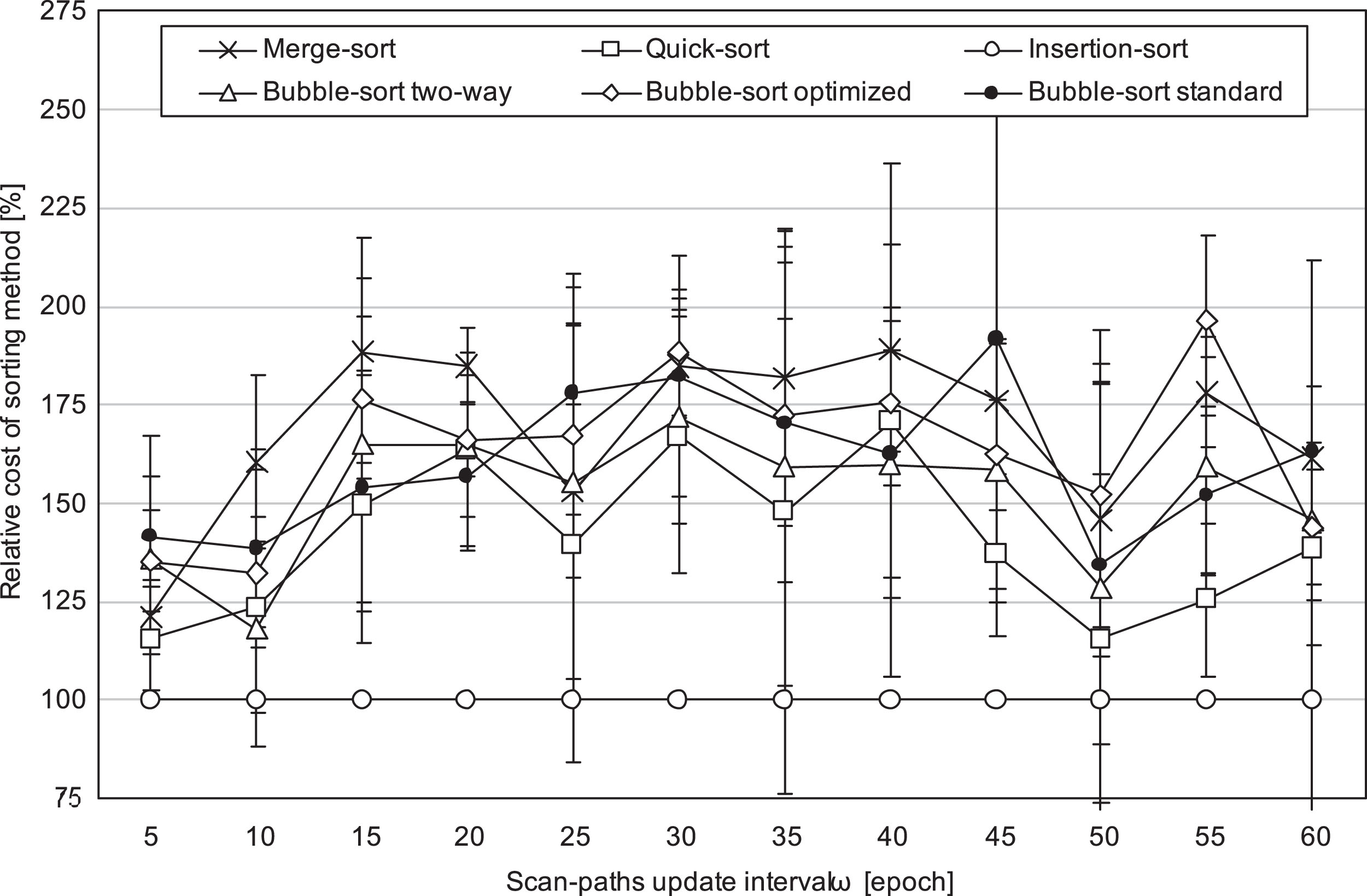
The mean relative cost of scan-paths sorting done while training of CxNN via the GBP for the Wines problem as a function of scan-paths update interval ω. The values are shown in relation to the outcomes for the ISort method. The activation function: the Exponential Rectifier. The stopping criterion: 300 epochs with non-decreasing error. The training step α = 0.01.

5 Conclusions

The results and evaluations described in this article are of unique character since the original error backpropagation method has no direct relations to sorting algorithms. The presented research concentrates on CxNNs with the Hard and Exponential Rectifier activation functions, what is an extension of analogous observations performed earlier for neural networks with the Bipolar Sigmoid and Leaky Rectifier activation functions [15].

We show that also for the Hard and Exponential Rectifier activation functions the scan-path evolution in contextual neurons under training is to a large degree affected by the self-consistency within the GBP. As a result, for scan-paths not longer than 30 items, the GBP algorithm is more computationally effective with the Insertion-sort than with other evaluated methods of sorting. The Quick-sort became a preferred option only for scan-paths exceeding this length, with the conclusion being valid across a vast spectrum of scan-path update intervals.

Previous measurements have shown that for Sigmoidal and Leaky Rectifier activation functions the threshold of scan-path length up to which the Insertion-sort should be used is 35 elements. Thus the different result obtained for Hard and Exponential Rectifier activations presents the fact that optimal selection of sorting methods for use with GBP should be based on complex relation with used activation functions. But in both observed cases the influence of self-consistency on the content of scan-paths is evident – the threshold for switching between Insertion-sort and Quick-sort during GBP is from 3 to 7 times greater than analogous values assumed in standard programming libraries. This arises from the fact that the scan-path-related data of contextual neurons remains partially sorted in the majority of GBP training epochs and that typical implementations of sorting methods are enhanced towards a maximum average performance for random data. Therefore, it is recommended to use fit-for-purpose sorting methods for updating the scan-paths of contextual neurons if the GBP computational efficiency is a significant factor.

The described experiments explore an interesting, earlier almost not analyzed subfield of ANN research. Further studies may encompass examinations of the GBP computational cost, including aspects such as optimized sorting methods (e.g. Shell-sort, Radix-sort, Tim-sort, partial interval sorting [19, 20]), novel functions of contextual aggregation or CxNNs’ and the parameters of GBP. Possible benefits of such further research include more efficient training of contextual neural networks in conjunction with an expansion of our current understanding of the very nature of such models.

References

Huk , Notes on the generalized backpropagation algorithm for contextual neural networks with conditional aggregation functions, Journal of Intelligent & Fuzzy Systems 32 (2017), 1365–1376. IOS Press.

Huk , Backpropagation generalized delta rule for the selective attention Sigma-if artificial neural network, Int J of App Math and Comp Sc 22 (2012), 449–459.

Huk , Learning distributed selective attention strategies with the Sigma-if neural network. In:

Akbar and

Hussain , (eds.) Advances in Computer Science and IT, InTech, Vukovar, 2009, pp. 209–232.

Szczepanik and

Jóźwiak , Data Management for Fingerprint Recognition Algorithm Based on Characteristic Points’ Groups, New Trends in Databases and Information Systems Advances in Int Systems and Computing, vol. 185, 2013, pp. 425–432. Springer.

Szczepanik and

Jóźwiak , Reliability and Error Probability for Multimodal Biometric System, Adv in Int Sys and Comp, Springer Berlin Heidelberg, 2014, pp. 325–332.

Huk , Measuring the Effectiveness of Hidden Context Usage by Machine Learning Methods under Conditions of Increased Entropy of Noise, In: 3rd IEEE International Confe-rence on Cybernetics, IEEE Press, 2017, pp. 1–6.

C.M.

Privitera ,

Azzariti and

L.W.

Stark , Locating regions-of-interest for the Mars Rover expedition, Int J of Remote Sensing 21 (2000), 3327–3347. Taylor & Francis.

Raczkowski and

Canning , Thomas-Fermi charge mixing for obtaining self-consistency in density functional calculations, Phys Rev B 64 (2001), 121101–121105. APS.

L.R.

Ram-Mohan ,

K.H.

Yoo and

Moussa , The Schrödinger–Poisson self-consistency in layered quantum semiconductor structures, Journal of Applied Physics 95(6) (2004), 3081–3092. AIP Publishing

10.

Glosser ,

Piermarocchi and

Shanker , Analysis of dense quantum dot systems using a self-consistent Maxwell-Bloch framework, In: Proceedings of 2016 IEEE International Symposium on Antennas and Propagation (USNC-URSI), Puerto Rico, IEEE, 2016, pp. 1323–1324.

11.

B.W.

Mel , The Clusteron: Toward a simple abstraction for a complex neuron, Advances in Neural Information Processing Systems 4 (1992), 35–42. Morgan Kaufmann.

12.

M.W.

Spratling and

Hayes , Learning synaptic clusters for nonlinear dendritic processing, Neural Processing Letters 11 (2000), 17–27.

13.

Glorot ,

Bordes and

Bengio , Deep sparse rectifier networks. In Proceedings of the 14th International Conference on Artificial Intelligence and Statistics, JMLR W&CP Volume, vol. 15, 2011, pp. 315–323.

14.

D.A.

Clevert ,

Unterthiner and

Hochreiter , Fast and Accurate Deep. Network Learning by Exponential Linear Units (ELUs), 4th International Conference on Learning Representations ICLR 2016, Puerto Rico, 2016, pp. 1–14.

15.

Huk , Weights Ordering. During Training of Contextual Neural Networks with Generalized Error Backpropagation: Importance and Selection of Sorting Algorithms. In:

N.T.

Nguyen ,

D.H.

Hoang ,

T.-P.

Hong ,

Pham ,

Trawiński (Eds.), Intelligent Information and Database Systems. Lecture Notes in Computer Science, vol. 10752, 2018, pp. 200–211. Springer.

16.

Knuth , The Art of Computer Programming: Sorting and Searching. vol. 3. Addison Wesley, 1998.

17.

J.L.

Bentley and

M.D.

McIlroy , Engineering a sort function, Software: Practice and Experience 23 (1993), 1249–1265. Wiley.

18.

Astrachan , Bubble sort: An archaeological algorithmic analysis, SIGCSE Bulletin 35 (2003), 1–5. ACM New York.

19.

P.M.

McIlroy , Optimistic Sorting and Information Theoretic Complexity, In: Proceedings of the Fourth Annual ACM-SIAM Symposium on Discrete Algorithms, 1993, pp. 467–474.

20.

P.M.

McIlroy ,

Bostic and

M.D.

McIlroy , Engineering radix sort, Computing Systems 6(1) (1993), 5–27.