On the stability and Lyapunov direct method for fractional difference model of BAM neural networks

1 Introduction

Fractional differential equations (FDEs) are perceived as indisputable models to nonlinear differential equations. The researchers have recently assimilated that FDEs have widespread applications in various fields of science and engineering such as engineering optimization and pattern recognition. Furthermore, FDEs are employed in social science such as food supply, climate and economics. Thus, the study of these equations has been the object of considerable scrutiny during the last decades. Meanwhile, different definitions for the concepts of differentiation and integration have been proposed and used to prove the qualitative properties of solutions of FDEs using various methods and diverse approaches [1–6].

The discretization of FDEs is of great antecedence for scholars who are interested in numerical analysis. In alignment with the fact that not all discrete operators acquire similar features as of the continuous ones, the investigation of discrete analogue of fractional calculus has become crucial topic. Consequently, some researchers have taken the lead and established the study of discrete fractional calculus and subsequently reported significant results on fractional difference equations (FdEs) which are the discrete correspondent of FDEs; see for instance [7–12]. Nevertheless and upon exploring the literature, one can figure out that the study of FdEs has comparably gained less attention among researchers than FDEs.

Due to their effective descriptions for processes which involve infinite memory, FDEs have been incorporated to investigate the neural networks with transmission delays. It has been found that BAM neural networks are entirely history dependent biological models which can be adequately expressed using FDEs involving discrete or distributed delays. Moreover, researchers have figured out that the existence of the delays in the process has direct backlash on its stability attitude. This has been the motivation that encourages them to study the behavior of solutions of fractional–order BAM neural networks and examine how the delays affects the process [13–19].

The stability of FDEs has recently attracted increasing interest amongst scholars. In [20], Matignon was the first who analyzed the stability of linear FDEs with Caputo derivative. Since then, many papers have been published on the stability of linear and nonlinear FDEs [21–24]. Lyapunov’s methods provide an efficient tool for stability analysis for nonlinear differential equations. There are several stability assesments combined with Lyapunov’s approach in the literature [25]. In his remarkable paper [26], Podlubny et. al. extended the Lyapunov direct method to the case of FDEs and proposed the concept of Mittag–Leffler stability for these equations. Thereupon, many researchers have consolidated the Mittag–Leffler stability into fractional–order BAM neural networks and thus obtained many noticeable results in this regard [27–31]. Never the less, one can notice that all the results obtained in the above listed papers have been conducted for continuous fractional–order operators. To the best of authors’ noticing, however, the progress regarding the investigation of stability results for FdEs and fractional difference neural networks is hardly considered; see the recent papers in this regard [32–34].

As previously stated, it is evident that not all properties of continuous operators are forfeited by the discrete counterpart operators. For instance, the α rising function t ^α for continuous operators, which have the property t ^α  + t ^β  = t^α+β, does not hold true for discrete operators. That is, t α ¯ + t β ¯ is not necessarily equal to t α + β ¯ . Motivated by the above discussion, the current authors find it imperative to investigate the following fractional difference system of BAM neural network. { c ∇ α x i ( t ) = − c i x i ( t ) + ∑ j = 1 m a i j f j ( y j ( t − τ ) ) + I i , i = 1 , 2 , … , n , c ∇ α y j ( t ) = − d j y j ( t ) + ∑ i = 1 n b j i g i ( x i ( t − τ ) ) + J j , j = 1 , 2 , … , m ,(1) where t ∈ ℕ 0 –the set of natural numbers including zero, 0 < α < 1 and ^c  ∇  ^α denotes the Caputo fractional difference operator of order α. Here x _i and y _j denote the potential (or voltage) of the cell at time t of the i–th neuron and the j–th neuron, respectively; f _j and g _i are the non-linear activation functions; I _i and J _j denote the i–th and the j–th component of an external bias; the positive constants c _i and d _j denote the strengths at which the i–th and the j–th cell reset their potential to the resting state when isolated from the other cells as well as from external inputs; a _ij and b _ji denote the strength of connections and τ is the non-negative discrete constant denoting transmission delay.

The initial conditions combined with system (1) are defined as

x i ( s ) = φ i ( s ) , y j ( s ) = ψ j ( s ) , s ∈ [ - τ , - τ + 1 , … , 0 ] , i = 1 , 2 , … , n , j = 1 , 2 , … , m ,(2) where φ i , ψ j ∈ I τ = B ( [ - τ , - τ + 1 , … , 0 ] , ℝ ) : the set of all bounded sequences defined on their domains. The investigation herein this paper are executed by using the nabla backward operator which stands in need to basic preparations on discrete backward fractional calculus.

The main goal of this work is to settle down sufficient conditions for the existence, uniqueness and global Mittag–Leffler stability of system (1)-(2). We will employ the newly defined discrete fractional calculus and implement the techniques of the Lyapunov function and Lyapunov direct method via discrete settings to prove the main results. We construct two examples to verify and illustrate the proposed theoretical findings.

For completeness, we briefly state some basic definitions and essential lemmas on discrete fractional calculus. These preliminaries serve as imperative foundations before proving the main results. We refer the readers to [33, 36] for proofs and justifications in this section.

Let ℝ be the set of real numbers, ℕ the set of natural numbers and ℕ 0 the set of natural numbers including zero. For any α ∈ ℝ , t ∈ ℝ \ { ⋯ , - 2 , - 1 , 0 } we define the α rising function as t α ¯ = Γ ( t + α ) Γ ( t ) , t ∈ ℝ \ { ⋯ , - 2 , - 1 , 0 } , 0 α ¯ = 0 ,(3) where Γ (·) denotes the Gamma function, which satisfies Γ (α + 1) = αΓ (α). The nabla backward difference of x is given by ∇ x ( t ) = x ( t ) - x ( t - 1 ) , t ∈ ℕ .

Definition 2.1. [35] Let x : ℕ 0 → ℝ , the backward jump operator ρ ( s ) : ℕ 0 → ℕ 0 defined as ρ (s) = s - 1. Then for α ∈ (0, 1) , the Riemann–Liouville’s sum operator of x is defined as ∇ - α x ( t ) = 1 Γ ( α ) ∑ s = 1 t ( t - ρ ( s ) ) α - 1 ¯ x ( s ) , t ∈ ℕ .(4)

Property 1. For μ > -1, we have ∇ - α t μ ¯ = Γ ( μ + 1 ) Γ ( μ + α + 1 ) t α + μ ¯ , t ∈ ℕ 0 .(5)

Definition 2.2. [35] Let x : ℕ 0 → ℝ and ρ (s) = s - 1. Then for α ∈ (0, 1) , the Riemann–Liouville’s difference operator of x is defined as ∇ α x ( t ) = ∇ ( ∇ 0 - ( 1 - α ) ) x ( t ) = ∇ Γ ( 1 - α ) ∑ s = 1 t ( t - ρ ( s ) ) - α ¯ x ( s ) , t ∈ ℕ .(6)

Definition 2.3. [35] Let x : ℕ 0 → ℝ and ρ (s) = s - 1. Then for α ∈ (0, 1) , the Caputo’s difference operator of x is defined as;

c ∇ α x ( t ) = ∇ 0 − ( 1 − α ) ∇ x ( t ) = 1 Γ ( 1 − α ) ∑ s = 1 t ( t − ρ ( s ) ) − α ¯ ∇ x ( s ) , t ∈ ℕ .(7)

Property 2. The Caputo’s difference of a constant function is zero.

Mittag–Leffler function is regularly employed in the theory of FDEs. Therefore, we recall herein its discrete fractional version.

Definition 2.4. [36] For λ ∈ ℝ , |λ|<1, and t ∈ ℂ –the set of complex numbers, the discrete fractional Mittag–Leffler function with one parameter is defined as E α ¯ ( λ , t ) = ∑ k = 0 ∞ ( λ ) k t k α ¯ Γ ( k α + 1 ) .(8) The discrete fractional Mittag–Leffler function with two parameters is defined as E α , β ¯ ( λ , t ) = ∑ k = 0 ∞ ( λ ) k t k α + β - 1 ¯ Γ ( k α + β ) , where α , β ∈ ℂ and Re ( α ) > 0 .

Definition 2.5. [36] Let f (t) be defined on ℕ 0 . Then, the discrete Laplace transform of f is given by L { f ( t ) } ( s ) = ∑ t = 1 ∞ ( 1 - s ) t - 1 f ( s ) .(9)

Lemma 2.1. [36] Let f (t) be defined on ℕ 0 and 0 < α ≤ 1. Then ( L ∇ α f ( t ) ) ( s ) = s α ( L f ) ( s ) - s α - 1 f ( 0 ) .

The Laplace transforms of Mittag–Leffler functions are essential in proving the main results.

Lemma 2.2. [36] For 0 < α ≤ 1 and f (t) defined on ℕ 0 , we have

( L { E α ¯ ( λ , t ) } ) ( s ) = s α - 1 s α - λ ,

Lemma 2.3. [37] If the Laplace transforms of f (t) and g (t) are F (s) and G (s) respectively, then L { ( f * g ) ( t ) } = F ( s ) G ( s ) , that is L - 1 { F ( s ) G ( s ) } = ( f * g ) ( t ) , where ^″ * ″ is called the convolution operator defined as ( f * g ) ( t ) : = ∑ r = 0 t - 1 f ( r ) g ( t - 1 - r ) , t ∈ ℕ 0 .

Consider the following delayed Caputo fractional order difference equation { c ∇ α x ( t ) = f ( t , x ( t ) , x ( t − σ ) ) , t ∈ ℕ 0 , σ ≥ 0 , x ( t ) = ϕ ( t ) , t ∈ [ − σ , 0 ] .(10)

Definition 2.6. The constant x^* is an equilibrium point of equation (10) if and only if f (t, x^*, x^*) =0 for any t ∈ ℕ 0 .

Definition 2.7. The trivial solution (or zero solution) of equation (10) is said to be asymptotic stable, if there exists a real positive constant δ = δ (0) >0 such that ∥ (φ) ∥ < δ implies that x (t) →0 as t→ ∞.

Denote the sup norm as ‖ φ ‖ : = sup t ∈ ℕ 0 | φ ( t ) | . We define the concept of stability in the sense of Mittag–Leffler as follows.

Definition 2.8. [33] The fractional difference equation (10) or the zero solution x of (10) is said to be Mittag–Leffler stable if ‖ x ( t ) ‖ ≤ m ( x ( t 0 ) ) E α ¯ ( λ , t ) , where α ∈ (0, 1) ,   - α < λ < 0, t₀ is the initial time of consideration, m (x (t)) is locally Lipschitz on discrete domain D with m (0) =0, m (x (t)) ≥0 and E α ¯ is the Mittag–Leffler function defined in (8).

Remark. It is clear that Mittag–Leffler stability implies asymptotic stability.

The class– K sequences are applied to analyze the fractional Lyapunov direct method. Thus, we need the following definition.

Definition 2.9. A bounded sequence β : ℕ 0 , t : = { 0 , 1 , 2 , … , t } → [ 0 , ∞ ) is said to belong to class– K if it is strictly increasing along with β (0) =0.

We assume that the following hypotheses are true throughout the remaining part of the paper.

The non-linear activation functions f _j  (·) and g _i  (·) are Lipschitz continuous with Lipschitz constants L f = max 1 ≤ j ≤ m { L f j } > 0 and L g = max 1 ≤ i ≤ n { L g i } > 0 .

Lemma 3.1. Assume that v (t) is a sequence defined on ℕ 0 with ∇ α v ( t ) ≤ - γ v ( t ) , α ∈ ( 0 , 1 )(11) for some constant γ where |γ|<1. Then v ( t ) ≤ γ 0 E α ¯ ( - γ , t )(12) where γ₀ = v (0).

Proof. In view of (11), there exists a non-negative sequence m such that ∇ α v ( t ) = - γ v ( t ) - m ( t ) . Let L { m ( t ) } ( s ) = M ( s ) and L { v ( t ) } ( s ) = V ( s ) . Then by using the discrete Laplace transform (9), we obtain s α V ( s ) - s α - 1 v ( 0 ) = - γ V ( s ) - M ( s ) or V ( s ) = s α - 1 s α - ( - γ ) v ( 0 ) - M ( s ) s α - ( - γ ) . The application of the inverse Laplace transform and the use of the properties of Lemma 2.2 and 2.3 yield that v ( t ) = E α ¯ ( - γ , t ) v ( 0 ) - m ( t ) * t α - 1 E α , α ¯ ( - γ , t ) . Since m and E α , α ¯ are non-negative functions, it implies that v ( t ) ≤ γ 0 E α ¯ ( - γ , t ) .

Theorem 3.2. Let hypotheses (H1)- (H3) be satisfied. Then the solution of fractional-order BAM neural network (1)-(2) exists and is unique.

The proof of the above statement is attained by employing the Krasnoselskii fixed point theorem. To avoid redundancy, however, we will omit the proof and refer the reader to Theorem 3.1 of [41].

We will employ the technique of the Lyapunov function to prove the Mittag–Leffler stability of system (1)-(2).

Theorem 3.3. Assume that the hypotheses (H1) is satisfied. Then the equilibrium (x^*, y^*)  ^T of (1)-(2) is Mittag–Leffler stable under the following condition: min { c * , d * } > max { sup i { | a i * | L f } , sup j { | b j * | L g } } > 0 ,(13) where c * = min i { c i } and d * = min j { d j } for i = 1, 2, ⋯ , n, j = 1, 2, ⋯ , m .

Proof. If (x^*, y^*)  ^T is the equilibrium point, then the error ( e , e ¯ ) = ( e 1 , ⋯ , e n , e ¯ 1 , ⋯ , e ¯ m ) T , where e i ( t ) = x i ( t ) - x i * , e ¯ j ( t ) = y j ( t ) - y j * satisfy the following system:

{ c ∇ α e i ( t ) = − c i e i ( t ) + ∑ j = 1 m a i j [ f j ( e ¯ j ( t − τ ) + y j * ) − f j ( y j * ) ] c ∇ α e ¯ j ( t ) = − d j e ¯ j ( t ) + ∑ i = 1 n b j i [ g i ( e ¯ i ( t − τ ) + x i * ) − g i ( x i * ) ] .(14)

We define the following Lyapunov function v ( t , e ( t ) ) = ∑ i = 1 n | e i ( t ) | + ∑ j = 1 m | e ¯ j ( t ) | .(15) For t ≥ 0, calculating the Caputo’s difference of v (t, e (t)) along solutions of (14), we obtain

c ∇ α v ( t , e ( t ) ) = ∑ i = 1 n c ∇ α | e i ( t ) | + ∑ j = 1 m c ∇ α | e ¯ j ( t ) | ≤ ∑ i = 1 n [ − c i | e i ( t ) | + ∑ j = 1 m | a i j | | f j ( e ¯ j ( t − τ ) + y j * ) − f j ( y j * ) | ] + ∑ j = 1 m [ − d j | e ¯ j ( t ) | + ∑ i = 1 n | b j i | | g i ( e i ( t − τ ) + x i * ) − g i ( x i * ) | ] ≤ ∑ i = 1 n [ − c i | e i ( t ) | + ∑ j = 1 m | a i j | L f j | e ¯ j ( t − τ ) | ] + ∑ j = 1 m [ − d j | e ¯ j ( t ) | + ∑ i = 1 n | b j i | L g i | e i ( t − τ ) | ] ≤ − min i { c i } ∑ i = 1 n | e i ( t ) | − min j { d j } ∑ j = 1 m | e ¯ j ( t ) | + ∑ i = 1 n ∑ j = 1 m | a i j | L f j | e ¯ j ( t − τ ) | + ∑ j = 1 m ∑ i = 1 n | b j i | L g i | e i ( t − τ ) | ≤ − k 1 v ( t , e ( t ) ) + sup i ( | a i * | L f ) ∑ j = 1 m | e ¯ j ( t − τ ) | + sup j ( | b j * | L g ) ∑ i = 1 n | e i ( t − τ ) | ≤ − k 1 v ( t , e ( t ) ) + k 2 ( ∑ i = 1 n | e i ( t − τ ) | + ∑ j = 1 m | e ¯ j ( t − τ ) | )(16)

Thus, we obtain

c ∇ α v ( t , e ( t ) ) ≤ - k 1 v ( t , e ( t ) ) + k 2 sup t - τ ≤ r ≤ t v ( r , e ( r ) ) ,(17) where k₁ = min {c^*, d^*} , and k 2 = max { sup i { | a i * | L f } , sup j { | b j * | L g } } . By considering the solution e (t) satisfying Razumikhin estimate v ( r , e ( r ) ) ≤ v ( t , e ( t ) ) , t - τ ≤ r ≤ t , we get c ∇ α v ( t , e ( t ) ) ≤ - ( k 1 - k 2 ) v ( t , e ( t ) ) , k 1 > k 2 . or c ∇ α v ( t , e ( t ) ) ≤ - γ v ( t , e ( t ) ) , where γ > 0. Using Lemma 3.1, we obtain v ( t , e ( t ) ) ≤ z ( 0 , e ( 0 ) ) E α ¯ ( - γ , t ) , or v ( t , e ( t ) ) ≤ m 0 E α ¯ ( - γ , t ) , where m₀ = v (0, e (0)) = {∥ x (t) - x₀ ∥ + ∥ y (t)- y₀ ∥} = { ∥ x (t) - φ₀ ∥ + ∥ y (t) - ψ₀ ∥ } > 0 and m₀ = 0 only if e (0) =0. Thus the solution is Mittag–Leffler stable.

In the following, we will prove the Mittag–Leffler stability of system (1). By virtue of the fact that any point can be shifted to the origin via a change of variables, we will consider the equilibrium point to be the origin. Let D ⊂ ℝ be a domain containing the equilibrium. Define the Lyapunov fucntion v ( t , e ( t ) ) : ℕ 0 × D → ℝ by (15).

Theorem 3.4. Let v be locally Lipschitz continuous with respect to x such that β 1 ‖ e ‖ ≤ v ( t , e ( t ) ) ≤ β 2 ‖ e ‖ ,(18) c ∇ α v ( t , e ( t ) ) ≤ - β 3 ‖ e ‖ ,(19) where 0 < α < 1, and β₁,  β₂  β₃ are arbitrary positive constants. Then the equilibrium (x^*, y^*)  ^T  = (0, 0)  ^T of system (1) is Mittag–Leffler stable.

Proof. In view of (18) and (19), we obtain c ∇ α v ( t , e ( t ) ) ≤ - β 3 β 2 v ( t , e ( t ) ) .(20) Then there exists a function m, which is non-negative such that c ∇ α v ( t , e ( t ) ) + m ( t ) = - β 3 β 2 v ( t , e ( t ) ) .(21) Taking the Laplace transform of both sides, we get s α V ( s , e ( s ) ) - s α - 1 v ( 0 , e ( 0 ) ) + M ( s ) = - β 3 β 2 V ( s , e ( s ) ) , where V ( s , e ( s ) ) = L { v ( t , e ( t ) ) } ( s ) and M (s) = L { m ( t ) } ( s ) . Thus, we have

V ( s , e ( s ) ) = s α - 1 s α + β 3 β 2 - 1 v ( 0 , e ( 0 ) ) - 1 s α + β 3 β 2 - 1 M ( s ) .(22)

If e (0) ≠0, then v (0, e (0)) >0. By using that v (t, e (t)) is locally Lipschitz continuous with respect to e and applying the inverse Laplace transform to both sides, we get

v ( t , e ( t ) ) = E α ¯ ( - β 3 β 2 , t ) v ( 0 , e ( 0 ) ) - m ( t ) * t α - 1 E α , α ¯ ( - β 3 β 2 , t ) .(23) Since m and E α , α ¯ are nonnegative functions, the above equation (23) can be rewritten as v ( t , e ( t ) ) ≤ m 0 E α ¯ ( - β 3 β 2 , t ) ,(24) where m₀ = v (0, e (0)) . Now substituting equation (24) into equation (18), we obtain. ∥ e ( t ) ∥ ≤ m ¯ 0 E α ¯ ( - β 3 β 2 , t ) ,(25) where m ¯ 0 = m 0 β 1 > 0 and m ¯ 0 = 0 holds if and only if e (0) =0 . This implies that the zero equilibrium is Mittag–Leffler stable.

Lemma 3.5. Let z (0) = w (0) and ^c  ∇  ^α z (t) ≥  ^c  ∇  ^α w (t) where 0 < α < 1. Then z (t) ≥ w (t).

Proof. It follows from the assumption ^c  ∇  ^α z (t) ≥  ^c  ∇  ^α w (t) that there exists a sequence m which is non-negative and satisfies c ∇ α z ( t ) = m ( t ) + c ∇ α w ( t ) .(26)

Taking the Laplace transform of equation (26) implies s α Z ( s ) - s α - 1 z ( 0 ) = M ( s ) + s α W ( s ) - s α - 1 w ( 0 ) , where L { z ( t ) } ( s ) = Z ( s ) and L { w ( t ) } ( s ) = W ( s ) . Since z (0) = w (0), it follows that Z (s) = s^-αM (s) + W (s) . Applying the inverse Laplace transform, we obtain z ( t ) = c ∇ - α m ( t ) + w ( t ) , where m (0) =0. Since m is a non-negative sequence, we end up with the desired result.

Theorem 3.6. Let v (t, e (t)) and class– K sequences β₁, β₂ and β₃ satisfy β 1 ( ‖ e ‖ ) ≤ v ( t , e ( t ) ) ≤ β 2 ( ‖ e ‖ ) ,(27) c ∇ α v ( t , e ( t ) ) ≤ - β 3 ( ‖ e ‖ ) ,(28) where 0 < α < 1. Then, the equilibrium (x^*, y^*)  ^T  = (0, 0)  ^T of system (1) is asymptotically stable.

Proof. Following from inequalities (27) and (28), we obtain c ∇ α v ≤ - β 3 ( β 2 - 1 ( v ) ) .(29) In virtue of Lemma 3.5, we have v (t, e (t)) ≥0 that v (t, e (t)) ≤ v (0, v (0)). Here, we review two cases.

Case.1: Suppose there exists a t₁ ≥ 0 satisfying v (t₁, e (t₁)) =0. Then from (27) we obtain that e (t₁) =0. It follows that e = 0 is the equilibrium of system (1) that e (t) =0 for t ≥ t₁.

Case.2: Suppose there exists a constant ɛ > 0 such that v (t, e) ≥ ɛ for t ≥ 0. It follows from v (t, e (t)) ≤ v (0, e (0)) that 0 < ɛ ≤ v ( t , e ( t ) ) ≤ v ( 0 , e ( 0 ) ) , t ≥ 0 .(30) Substituting (30) into (29) gives, - β 3 ( β 2 - 1 ( v ( t , e ) ) ) ≤ - β 3 ( β 2 - 1 ( ɛ ) ) = - β 3 ( β 2 - 1 ( ɛ ) ) v ( 0 , e ( 0 ) ) v ( 0 , e ( 0 ) ) ≤ - χ v ( t , e ) , where χ = β 3 ( β 2 - 1 ( ɛ ) ) v ( 0 , e ( 0 ) ) > 0 . It follows that c ∇ α v ( t , e ( t ) ) ≤ - β 3 ( β 2 - 1 ( v ( t , e ) ) ) ≤ - χ v ( t , e ) . Following the similar arguments as in Theorem 3.4, we reach to v ( t , e ) ≤ v ( 0 , e ( 0 ) ) E α ¯ ( - χ , t ) . This contradicts the assumption that v (t, e) ≥ ɛ. The consequences obtained in Case 1 and Case 2 imply that v (t, e) →0 as t→ ∞. It follows from (27) that lim t → ∞ e ( t ) = 0 .

Remark. If the assumptions of the above theorems hold globally on ℝ n , then the equilibrium is globally Mittag–Leffler stable.

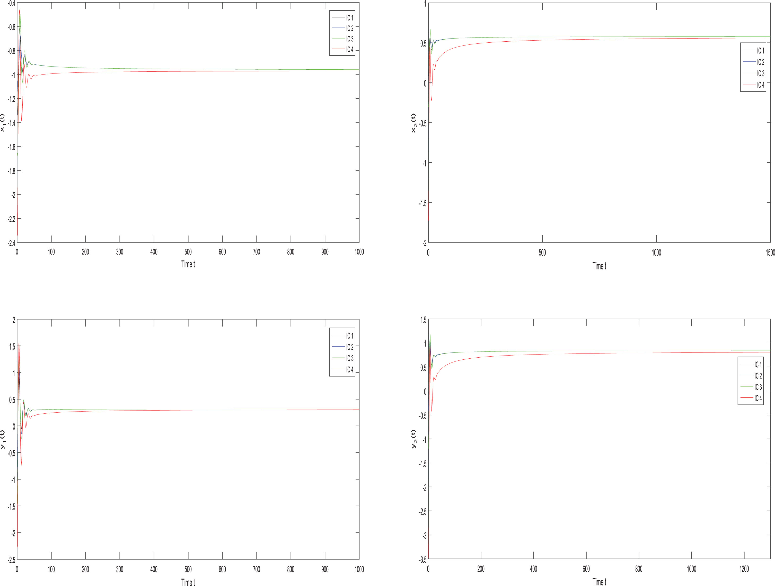
Example 1. Consider the following system { c ∇ α x 1 ( t ) = − 5 x 1 ( t ) + 0.1 tanh ( y 1 ( t − τ ) ) + 0.2 tanh ( y 2 ( t − τ ) ) − 5 , c ∇ α x 2 ( t ) = − 4 x 2 ( t ) + 0.4 tanh ( y 1 ( t − τ ) ) + 0.3 tanh ( y 2 ( t − τ ) ) + 2 , c ∇ α y 1 ( t ) = − 5 y 1 ( t ) + 0.2 tanh ( x 1 ( t − τ ) ) − 0.5 tanh ( x 2 ( t − τ ) ) + 2 , c ∇ α y 2 ( t ) = − 4 y 2 ( t ) − 0.3 tanh ( x 1 ( t − τ ) ) + 0.3 tanh ( x 2 ( t − τ ) ) + 3.(31) This corresponds to system (1) with α = 0.8, τ = 0.04 . The activation functions are chosen as f _j  (·) = g _i  (·) = tanh(·) ,  i, j = 1, 2 . The equilibrium point of system (4) is ( - 0.9663063805 , 0.5823883466 , 0.3176770173 , 0.8453606868 ) T . Furthermore, we have L _f  = L _g  = 1, and min i , j {c _i , d _j } = min {5, 4} =4 . Moreover, one can easily find that max { sup i { | a i * | L f } , sup j { | b j * | L g } } = 0.5 . Thus, condition (13) of Theorem 3.3 is satisfied. Hence, the equilibrium of system (4) is globally Mittag–Leffler stable and hence asymptotically stable. Figure 1 illustrates the trajectories of variables x _i  (t) and y _j  (t) of system (4) for t ∈ [-0.04, 0] . The following set of initial values is considered in simulation:

(φ₁ (t) , φ₂ (t) , ψ₁ (t) , ψ₂ (t))  ^T  = (0.5, 1.5, 5, 5)  ^T ,

OPEN IN VIEWER

Fig.1

The state trajectories of stable solutions of (31).

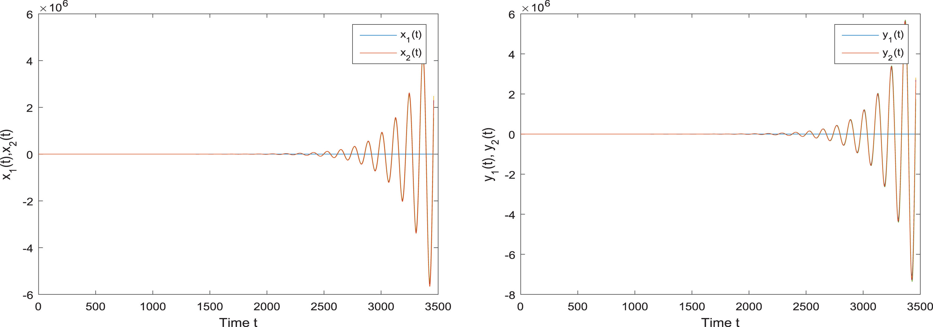
Never the less, we observe that if we change the coefficients c _i , d _i such that min i , j { c i , d j } = 1 and the time delay value as 0.5 with similar initial conditions, then the condition (13) of Theorem 3.3 is not satisfied. In this case, the solution loses its stability and becomes divergent. This behaviour can be depicted via Fig. 2:

OPEN IN VIEWER

Fig.2

The state trajectories of unstable solutions of (4).

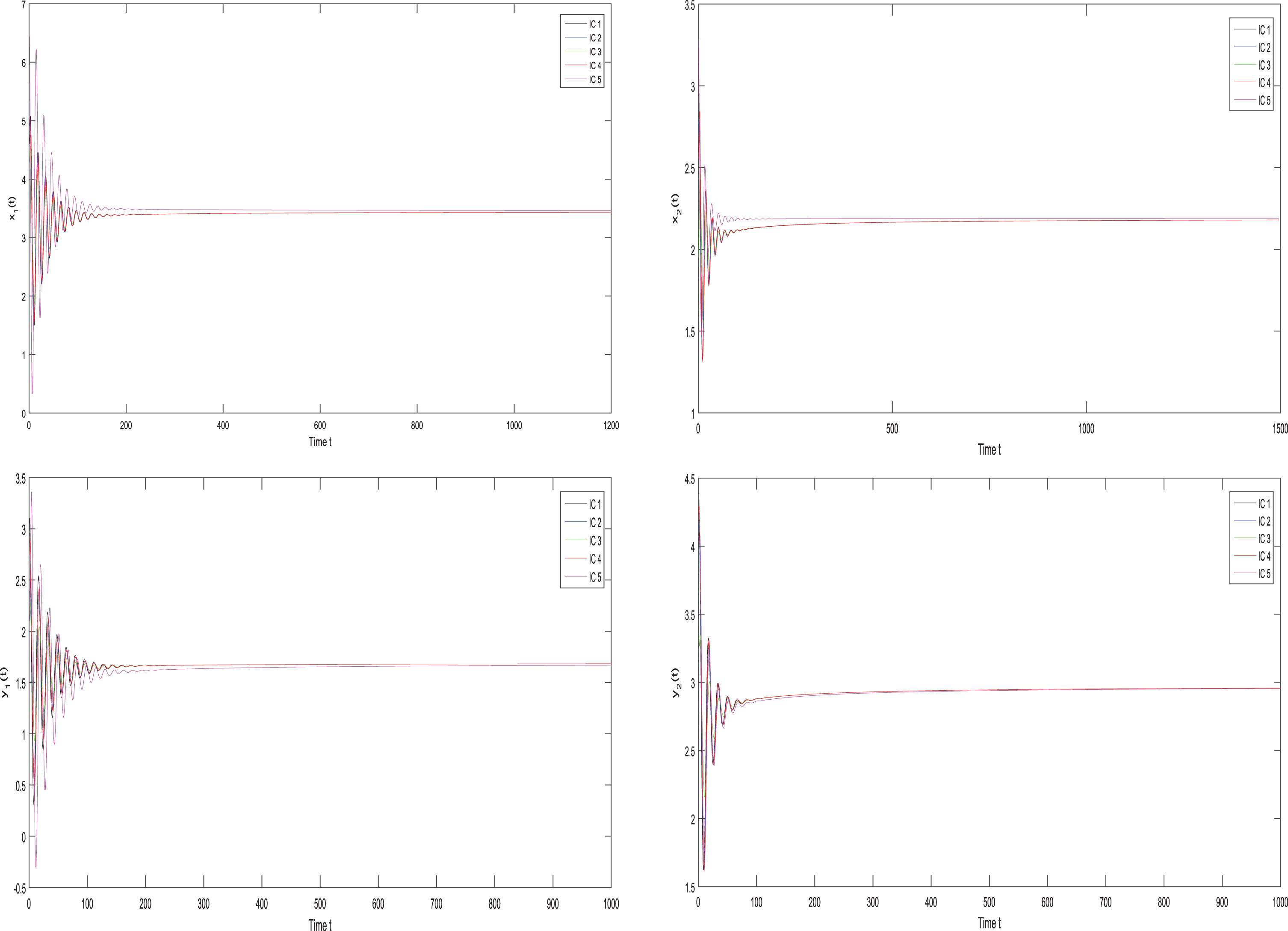
Example 2. Consider the following system with different activation functions; { c ∇ α x 1 ( t ) = − 6 x 1 ( t ) + 0.5 f 1 ( y 1 ( t − τ ) ) + 0.25 f 2 ( y 2 ( t − τ ) ) + 20 , c ∇ α x 2 ( t ) = − 5 x 2 ( t ) + 0.6 f 1 ( y 1 ( t − τ ) ) + 0.4 f 2 ( y 2 ( t − τ ) ) + 10 , c ∇ α y 1 ( t ) = − 6 y 1 ( t ) + 0.45 g 1 ( x 1 ( t − τ ) ) − 0.3 g 2 ( x 2 ( t − τ ) ) + 10 , c ∇ α y 2 ( t ) = − 5 y 2 ( t ) − 0.3 g 1 ( x 1 ( t − τ ) ) + 0.2 g 2 ( x 2 ( t − τ ) ) + 15 ,(32) where α = 0.9 and τ = 0.03 . The activation functions are g i ( x i ) = | x i + 1 | - | x i - 1 | 2 , and f _j  (y _j ) = | y j + 1 | - | y j - 1 | 2 , i , j = 1 , 2 . The equilibrium point for system (32) is ( 3.452659897 , 2.191727143 , 1.692749280 , 2.979133909 ) T .

Thus L _f  = L _g  = 1 . Furthermore min i , j { c i , d j } = 5 > max { sup i { | a i * | L f } , sup j { | b j * | L g } } = max {0.6, 0.3} =0.6 . Thus, condition (13) is fulfilled. Following Theorem 3.3, the equilibrium is globally Mittag-Leffler stable and hence asymptotically stable. The simulation results are shown for t ∈ [-0.03, 0] in Fig. 3. We consider the following set of initial values:

(φ₁ (t) , φ₂ (t) , ψ₁ (t) , ψ₂ (t))  ^T  = (3.5, 1.5, - 1.5, - 1.5)  ^T ,

OPEN IN VIEWER

Fig.3

The state trajectories of stable solutions of (32).

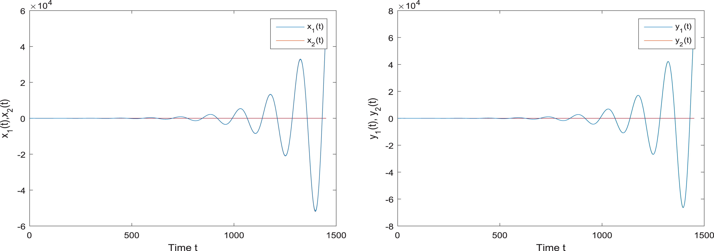
However, if we change the coefficients c _i , d _i such that min i , j { c i , d j } = min { 1 , 2 } = 1 and the time delay value as 0.5, then it violates condition (13) of Theorem 3.3. Hence the solution is not Mittag-Leffler stable. Figure 4 depicts the unstable behaviour of the solution of system (32).

OPEN IN VIEWER

Fig.4

The state trajectories of unstable solutions of (32).

This paper studies stability results for the fractional difference BAM neural networks. Particularly, sufficient conditions are established for the existence, uniqueness and global Mittag–Leffler stability for the nontrivial solutions of the addressed system. The newly established discrete fractional calculus are used to set the problem. We employ the techniques of the Lyapunov function and Lyapunov direct method in the frame of discrete fractional calculus to prove the main results. We believe that the investigation of neural networks in discrete fractional settings will lead to a better understanding of fractional dynamics. We have considered Caputo fractional derivative with nabla backward differences in this work. For future consideration, we will try to explore the opportunity to utilize different types of definitions of fractional differentiation and integration to prove results related to stability, almost periodicity and control.