
Abstract
The main motive of this work is to discriminate a vital neurodegenerative condition of Parkinson Disease (PD) affected patients from individuals with no history of such a disorder. Excitation source features, voice quality features and prosodic features are the speech constituents considered. Voice samples of PD patients are extracted from the University of California-Irvine (UCI) Machine Learning Parkinson’s database. Random Forest (RF) decision trees and Support Vector Machine (SVM) are considered for classification. Feature reduction is applied with the Correlation based Feature Selection (CFS) attribute selector classifier that utilizes Best First Selector (BFS) as a search algorithm. The work involves recognizing a PD patient from a healthy individual using only two speech sounds of /a/ and /o/. The speech sounds are extracted without the association of a certified clinician, that adds novelty. The proposed algorithm is non-invasive and accomplished 94.77% accuracy with feature selection process and applying RF classifier.
Keywords
Introduction
Degenerative disorder is a continuous phenomenon based on degenerative cell changes. Involvement of the central nervous system results in neurodegenerative (ND) disorder. Alzheimer’s disease, Parkinson’s disease (PD), Osteoporosis, Multiple sclerosis etc are among the most common ND disorders faced by the human community in the present day. PD is the second basic ND turmoil after Alzheimer’s. Hence, this work is focused on PD detection. PD is a disorder that affects neurons in the brain which influences about 10 million individuals around the world. Because of moderate, continuously dynamic nature of the confusion, PD has a prodromal interim amid which the fundamental engine signs are not plainly obvious [1].
Various methods for identifying PD is through speech extraction, Ultra High Frequency (UHF) detection and optical methods. The objective of this analysis is to identify PD at primitive stages [19].
Speech is chosen in this analysis since it is savvy, cost-effective and the presence of a clinician is not required. This study has detected PD through speech signals. The primary vocal hindrances because of PD is dysphonia. Dysphonia is the failure to create ordinary vocal acoustic sounds, and dysarthria, i.e., were not really ready to articulate words. Both dysarthria and dysphonia are related with diminished vocal din, precariousness and recurrence variation from the norm. On the other hand, hypertonia, which moreover happens in PD individuals, can hindered vocal quality and prompt voice break. Dysphonic measurements can help the appraisal of vocal debilitations because of PD, in this manner being very viable biomarkers to help its finding [2].
Ongoing analysis have raised the significant point of finding a statistical mapping between speech properties and detection of Parkinson disease [18, 20]. The conventional methodology for identifying PD involves use of range of basic linear and non-linear signal processing methods to compute acoustic features as an input for the classification algorithms [2, 21]. The dataset usually contains sustained vowels, consonants, words or alpha numerical characters.
The commonly used classification techniques and algorithms are Support Vector Machine (SVM) [3, 4], Random Forest (RF) [5], Multi-Layer Perceptron (MLP) [2], and Deep Multi-Layer Perceptron. K-Nearest Neighbor (KNN) [6]. Cross validation techniques such as Leave One Subject Out (LOSO), Summarized Leave-One-Out (S-LOO) [6] and K- fold cross validation have been applied. This work contributes a strategy to classify PD from healthy individuals by extracting significant excitation source features from the voice samples with the classification performed using RF and SVM.
This work contributes a strategy to classify PD from healthy individuals by extracting significant excitation source features from the voice samples with the classification performed using RF and SVM. This paper is arranged into 5 distinct sections. Section 2 explores the literature review for the detection of PD. Section 3 depicts the proposed algorithm. Section 4 states the background work accomplished before the analysis. Section 5 is focused on the results and analysis. Finally, Section 6 comprises of conclusion and future scope.
Literature survey
In the work proposed by M.A Little et al., accuracy achieved is remarkable (7.5 Unified Parkinson Disease Rating Scale (UPDRS) points difference from the clinicians’ estimates). UPDRS is the commonly used measurement for clinician to measure Parkinson. UPDRS comprises of three areas: 1) activities of daily living; 2) motor and 3)mentation, behaviour, and mood; [2]. Luca Parisi,et al., developed a new hybrid algorithm combining Multi-Layer Perceptron(MLP) and Lagrangian support vector machine(LSVM) with back propogation and 20 fold cross validation techniques. The hybrid algorithm had achieved a classification accuracy using least possible epochs (iterations N = 3) and computational time (0.01 s) [8]. B. E. Sakar et al., employed k-nearest neighbor (k-NN) and SVM as classification techniques. The classification performance of Summarized Leave-One-Out (S-LOO) validation technique is compared with LOSO technique and it is proved that highest accuracy of 77.50% which is achieved with S-LOO method [6].
Zhennao Cai et al., developed a new hybrid framework for detection of PD which mainly focuses on predicting PD accurately. The results have shown that the BFO-SVM framework exhibited excellent with an classification accuracy of 97.42% [3]. Similarly, Musaed Alhussein et al., created a cloud based framework which use speech signals captured from applicant via sensors and transmitted the captured signals to the cloud. In the cloud, decisions are made utilizing SVM classifier. He achieved around 97.2% accuracy [4]. Shaohua Wsn et al., proposed a deep multi-layer perceptron (DMLP) classifier to appraise the movement of PD utilizing cell phones. Main aim is to recognize seriousness in PD patients’ activities by dissecting their speech and development designs, as estimated with a cell phone accelerometer [9]. In their work, Max A. Little test how accurately the novel algorithms can be used to discriminate PD subjects from healthy individual. In total, 132 dysphonia measures are computed from vowels and used two binary classification response: random forests and support vector machines for classification [5].
Achraf Benba et al., has distinguished two groups of patients i.e. patients who are effected with PD and patients who are effected with other neurological disorders. Later on, analysed and features were extracted from the voice samples using different Cepstral techniques; perceptual linear prediction (PLP), ReAlitive SpecTrAl PLP (RASTA-PLP)and Mel frequency cepstral coefficients (MFCC) and achieved 90% with 11 coefficients of the linear SVM kernels and PLP [10].
Researchers have faced many bottlenecks while diagnosing Parkinson disease through speech. The major issue which was faced is that the pronounced vocal symptoms are prominently visible only at later stages of the disease. Hence few studies suggest that identification on PD at early stage accurately is a complex task.
Few studies usually take the help of clinicians to accurately identify the Parkinson disease through Unified Parkinson Disease Rating Scale (UPDRS). Identifying PD through UPDRS is a costly [2]. The biggest limitation is to overcome gender imbalance. The dataset should contain a good mix of both the genders, else the results would be biased. The crux of the problem lies in how the voice samples are recorded and the tools used for recordings.
In this work, is has been addressed that, instead of UPDRS score, non-linear dynamical speech processing methods and MFCC can be used to accurately identify the PD in the absence of a clinician. It is also proved that /a/ and /o/ vowels speech samples contain the required vocal tract information for the detection of PD. The significant features required for the detection of PD are identified through feature selection, which is discussed in section 5.The proposed algorithm in this work is discussed in the next section.
Proposed algorithm
The methodology employed in this work is illustrated in Fig. 1. The algorithm proposed is divided into 5 modules. Module 1 and 2 describes data acquisition and pre-processing steps. Module 3 deals with feature extraction of basic linear and nonlinear dynamical features while Module 4 and 5 deals about feature reduction and classification.
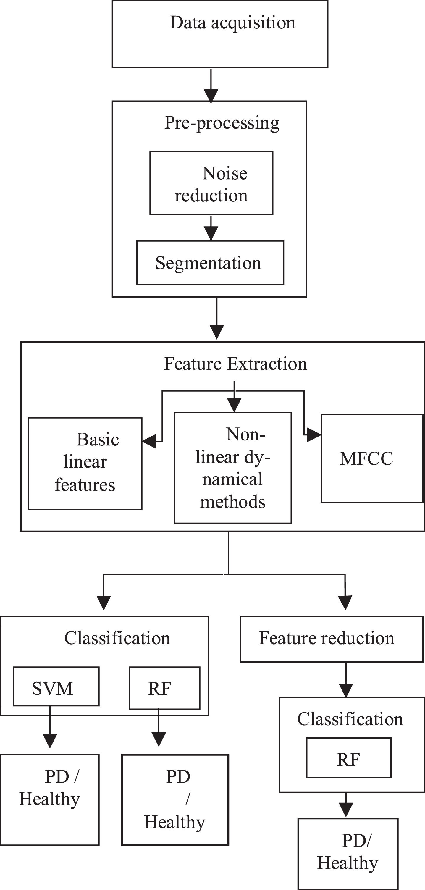
Proposed Algorithm.
The dataset consisting of a total of 176 samples were extracted from the UCI Machine Learning repository from Sakar et al. [6] and stored in.wav format. The repository has the information on sustained vowels and UPDRS score from the clinician (UPDRS: 13±15.89) of 28 subjects, with average age of 64.86±8.97 years; (gender: 6 females, 14 males) The dataset could be divided into two parts. Part 1 for PD patients and part 2 for healthy individuals. Part 1 for PD dataset was a questionnaire between PD patient and speaker. The PD patient was asked to pronounce /a/ and /o/ syllable for multiple times. The voiced and unvoiced part were separated by listening to the voice samples.
Part 2 contains the dataset of healthy individuals. The samples for healthy group were recorded via a smartphone. The healthy group was comprised of 18 volunteers with no history of any neurological disease. These Healthy group (age: 41.75±8.34 years; gender: 4 males and 14 females). Speech features from 89 samples were inspected around 44.1KHz and each of duration 5–6 seconds.
Pre-processing
From the speech recordings it has been analyzed that the database is made in the presence of a clinician who is assisting PD patients to repeat /a/ and /o/ vowels. Each speech recording has been analyzed and only /a/ and /o/ speech samples of PD are extracted. Stereo to mono channel conversion and noise reduction was also performed in audacity. After generating the feature vector for all the samples, the input features were standardized by plotting their base and peak values in the scale of 0 and +1 for all the separated list of capabilities. The development of a few algorithms for feature extraction was performed [6].
Feature extraction
Feature extraction is applied to reduce the amount of resources to describe the large dataset. The features extracted are the attributes to the classifier to determine PD. To extract basic linear features from the recordings praat acoustic analysis software was used and non-linear dynamical features were extracted by MATLAB (R2017b, The MathWorks, Inc.) [9]. Speech features extracted in this work are described as follows:
Basic linear features
3.3.1.1. Jitter and Shimmer
Jitter is the short duration period-to-period variation of peak-to-peak amplitude in speech. Jitter usually is the rough sound in the voice. It is because of the varying pitch in voice. Jitter is usually a deviation from the periodic signal.
Shimmer is amplitude variation (louder to soft) in voice. Shimmer is generally a variability in peak-to-peak amplitude in considered voice sample whereas jitter is variability in pitch period [11].
3.3.1.2. Pitch
Pitch is an acoustic measure that’s a relative measure of highness or lowness of the tone in the voice as perceived by the human ear. It is generally a measure of vibrations per second. In mathematics pitch is the inverse of the fundamental frequency. It’s is one of the major acoustic feature of intonation and tone [11].
3.3.1.3. Auto correlation
Correlation of the signal with itself after a time lag. It is the similarity between observations. It is a usually used for detect fundamental frequency or repeating patterns, or noise in the voice. In mathematics it usually finds the number of reputations or patterns in the signal [11].
3.3.1.4. Number of voice breaks
The quantity of detachments between consecutive pulses that are longer than 1.25 apportioned by the pitch floor. Henceforth, if pitch floor is 75 Hz, all between heartbeats intervals longer than 16.67 ms are seen as voice breaks [12].
3.3.1.5. Harmonic to noise ratio
HNR is a measure that evaluates the measure of additive noise in the speech sample [11].
Non linear dynamical features
3.3.2.1. Mel-frequency cepstral coefficients (MFCC)
MFCC is the Discrete Cosine Transform (DCT) of the power spectrum of a voice test on a nonlinear mel scale recurrence [13, 23].
3.3.2.2. Recurrence period density entropy (RPDE)
The RPDE tends to the capacity of the vocal folds to support straightforward vibration, measuring the deviations from precise periodicity [2].
3.3.2.3. Detrended fluctuation analysis (DFA)
DFA describes the degree of fierce clamour in the voice, measuring the stochastic self-similitude of disturbance brought about by violent wind stream in the vocal voice tract [2].
3.3.2.4. Pitch period entropy (PPE)
Pitch period is an time domain analysis of pitch at a period of time. Entropy of a system defines the randomness involved in a system. Pitch period entropy defines variation of pitch period of a signal in time domain for a particular duration of time [12].
Feature reduction
Dimensionality reduction is the way toward reducing the quantity of random features under consideration, by getting a set of principal variables [7]. The evaluator selected in Waikato Environment for Knowledge Analysis (WEKA) for feature reduction is performed using Attribute Selector Classifier with sub classifier as RF, correlation based feature selection (CFS) evaluator and search method used was Best First (BFS) in WEKA [22]. CFS evaluates the weight of each feature analysing the prescient capacity of each feature and the measure of repetition between them. Within a class, the features subset are highly correlated and between 2 classes there is minimal amount of correlation. The idea of Best First Search method is to use an evaluation function to decide which adjacent node in a tree or graph is most promising and then explore.
Classifier
In this work classification for the obtained feature set is done utilizing Support Vector Machine (SVM) and Random forest (RF) classifiers. The main aim of SVM classifier is to find a hyper plane which corresponds to an N – dimensional space which distinctly identifies all the features. To separate different features of data points we can have different kinds of hyper planes. But we need to find the plane which gives us a better margin. Support vectors are the features that are generally closer to the hyper plane. They usually define the orientation and position of the hyper plane. With the support of the support vectors we can maximise the margin of the classifier. In practical applications, information regularly can’t be linearly separated. Hence, SVM utilize the kernel trick to manipulate the information to a higher dimensional and build the separating hyper plane in that space. This paper use linear kernel type (gamma = 0.005 and cost = 10). All the conceivable mixes were consolidated to acquire better outcomes [6].
Random Forest is the best supervised learning algorithm. It utilizes multiple decision tree which are built in a haphazard way to solve the classification and regression problems. RF has the same hyper parameters as a decision tree. RF adds randomness into the model. Each and every decision tree in the RF constructs subset by considering random voice samples from the available feature set. While growing the trees the most important feature is not searched while splitting the nodes instead it finds the best feature among the available features. RF works better than a single decision trees as we take many decision trees into consideration. It also overcomes the shortcomings to over fitting. They can manage continuous and discrete feature set and are highly immune to noise. Using RF it is rather a simple task to measure the relative importance of each and every feature in from the feature set [5].
Evaluation metrics
In this work precision, accuracy and F-measure are used as evaluation metrics to analyze the system performance. Precision (P) – The absolute number of accurately characterized positive features by the complete number of predicted positive features [14]. Accuracy (A) – The rate of classification over all the given samples is called Accuracy [14]. F-Measure (F.M) – F-measure which uses Harmonic Mean to extend the range of the extreme values [14].
Experimental background
Speech features considered in this work are listed in Table 1. The feature sets are divided into three groups namely basic linear features, non-linear dynamical features and MFCC coefficients, to learn the contribution of different feature sets in the detection of PD, which adds novelty to the work in finding significant features even before the feature reduction. The total count of basic features is 24, non-linear dynamical features is 3 and MFCC coefficients are 42. Hence a total of 69 features are extracted. The number of coefficients extracted for each of the groups are mentioned in Table 2. Basic linear features are divided into 6 sections and nonlinear dynamical features are segregated in 3 groups. The feature sets are extracted from MATLAB (R2017b, The Math Works, Inc.) [2] and praat acoustic analysis software [12]. In this work, 5-fold cross validation technique is used to analyses the system performance [15, 16].
List of features
List of features
List of feature set
Various feature sets and the number of coefficients for each feature set are shown in Table 2. Among different sets, feature set 1 contains least number of features with 24 coefficients and feature set 10 containing the highest number of features with 69 coefficients. All the linear features are extracted in praat software [20] whereas, non-linear dynamical features and MFCC are extracted in Matlab [1].
Feature vector
A feature vector is a matrix of one or more column and rows which are represented spatially. Feature vectors are generally used practicality and effectiveness of representing spatially. They form good analysis while comparing different feature vectors. Feature vectors are compared using Euclidian distance [17]. For feature set 1 the feature vector is [1×24]. For feature set 2 the feature vector is [1×66] and similarly for all the feature sets, the size of the feature vector is [1×number of coefficients].
Results and analysis
As an initial work, all the feature sets that are listed in Table 2 have been analysed and the feature vectors are constructed for all the feature sets. As a pre-processing step, the input features were standardized by plotting their base and peak values in the scale of 0 and +1 for all the feature sets using Weka [7]. The experimental work involves classification of all the feature sets and the comparative performance is analysed for all of them. Here, SVM and RF classifiers are employed for classification and the performance of the system is compared with both the classifier, where a cross validation of 5-folds is employed during the classification. The experiment is performed at 4 levels which are listed below and will be discussed further in detail.
Performance analysis of all the feature sets using SVM classifier
After constructing different feature sets using the combinations in Table 2, each feature set is classified with SVM classifier. Performance comparison is carried out for all the feature sets to observe the contribution of different features in the classification. Table 3 represents the classification performance obtained using each feature set in the detection of PD, using SVM classifier with parameters containing kernel type linear, gamma value of 0.005 and regularisation or cost parameter having a value of 10.
Performance analysis using SVM and RF
Performance analysis using SVM and RF
From Table 3, it can be incurred that with only linear features accuracy achieved is only 79.62% as the number of coefficients are only 24. With the addition of MFCC features the accuracy reached to 90.94% as the number of coefficients used in MFCC are 42 and the total number of coefficients employed are 66. It can be observed that with only the non-linear dynamical methods used in combinations of one or two and linear features, average accuracy achieved is 81.12% because extra coefficients added are only one or two. So there is no much difference in the accuracies for the feature sets with linear features and different non-linear dynamical methods.
When all the non-linear dynamical features are used at a time with the combination of linear features, there is an increase of 2% in the accuracy and it has reached up to 83%. Finally, with the combination of all extracted features, a maximum accuracy of 93.2% with precision and f-measure as 93.2% and 93.2% respectively, have been achieved with SVM.
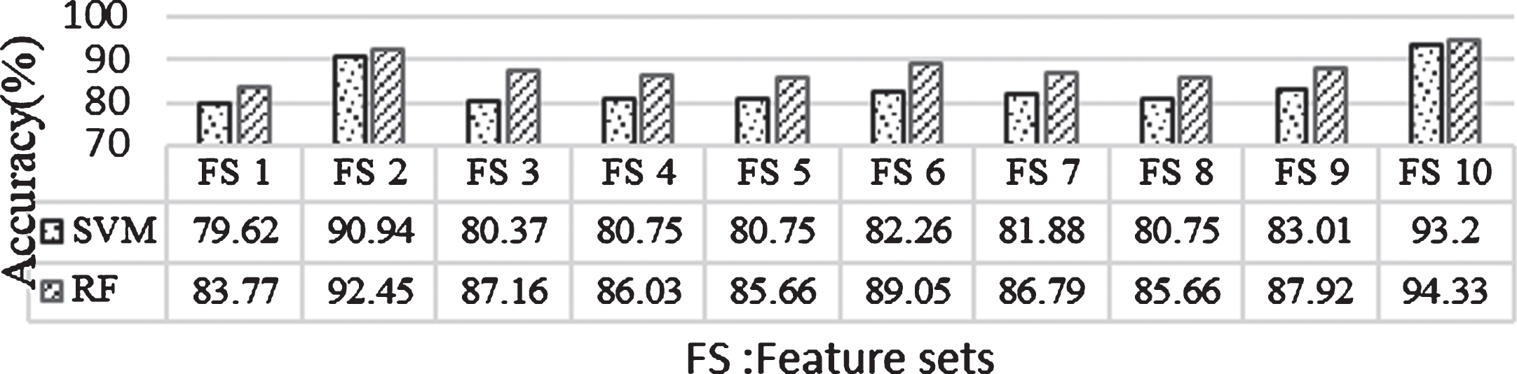
The next task involves analyzing the classification performance for all the 10 feature sets using RF classifier. From Table 3, it can be incurred that an overall accuracy of 94.33% is obtained with RF classifier with the feature set 10 containing a total no of 69 coefficients. As in SVM, the second highest accuracy of 92.45% is obtained with feature set 2 as the total no. of coefficients are 66.
With the feature sets containing combinations of non-linear dynamical features and linear features, an average accuracy of 86.89 % is obtained as the total no. of co-efficients used are around 25. The best accuracy of 89.05% with precision and f-measure as 89.1% and 88.8% respectively, are achieved with the combination of PPE and DFA features even though the total no. of coefficients are only 26 in that feature set. As observed from the Table 3, better performance is obtained with feature set 10. Hence forth feature set 10 is referred as the proposed feature set in the following sub sections.
Comparative performance of SVM and RF using proposed technique
Here, using the proposed feature set, performance of the system using SVM and RF classifiers are analyzed. From Fig. 2, it can be observed that RF classifier has produced better results than SVM classifier for all the employed feature sets. When all the extracted features are used at a time i.e., in the case of proposed features set, it is noticed that there an increase of only 1.13% in accuracy with RF than in SVM. With only MFCC coefficients both the classifiers are producing an average accuracy of 91.69 %, whereas 90.94% is noticed in SVM and 92.45% from RF. In all other cases, there is an average increase of 5.33% in accuracy with RF than in SVM.
Comparative performance analysis of SVM and RF Classifiers using proposed feature set.
It is noticed that the best classification performance is attained with the feature set 10, containing 69 coefficients where 42 coefficients belong to MFCC, 3 coefficients are from 3 non-linear dynamical methods respectively and 24 coefficients are from linear features group. A feature set with 69 attributes or coefficients is complex to analyse and can lead to misclassification also. All the 69 coefficients may not play a significant role in the classification. So feature reduction is a required method to minimize the dimensionality of the feature vector and computational cost and time, and to obtain a compact feature set, which will be discussed in the following section.
As mentioned in Section 3.4, feature reduction is done using attribute selection classifier with RF, CFS subset evaluator and Best first search method. The classification performance is analysed before and after feature reduction. Figure 3 illustrates the comparative performance analysis obtained with both the feature sets. An accuracy of 94.72%, precision of 94.8% and f-measure 94.7% is achieved with the reduced feature set as against the proposed feature set yielded an accuracy of 94.33%, precision of 94.8% and f-measure as 94.7%. It is noticed that the feature reduction has not only increased the accuracy by 0.39% but also reduced the computational cost, spatiality of the feature set and identified the significant features in the detection of PD.
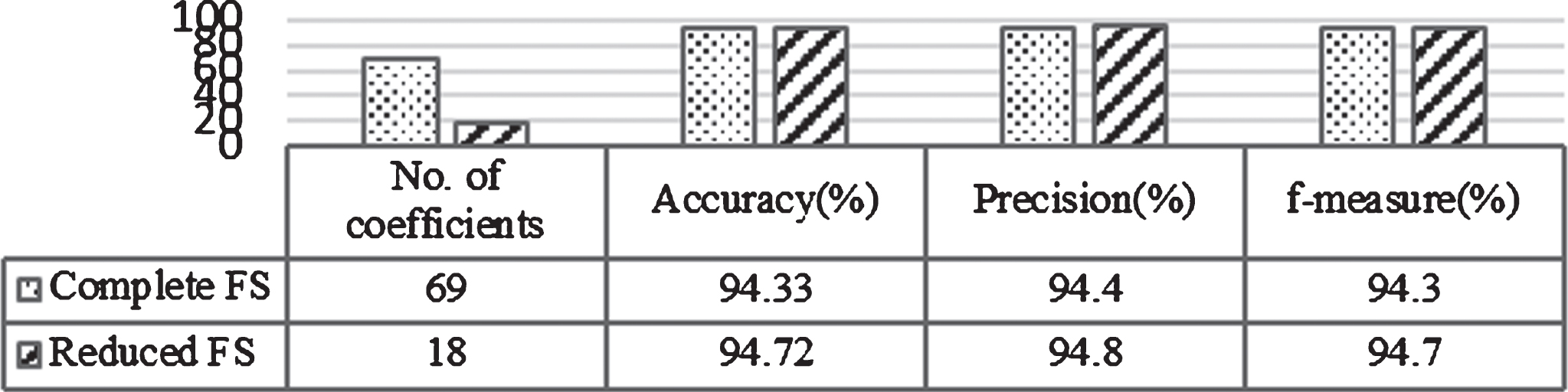
Performance analysis for proposed feature set and reduced feature set.
After feature reduction, it has been found that the reduced feature set contains only 18 features, which are found to be significant features in the detection of PD.
Among all the extracted features, number of pulses, standard deviation of period, number of voice breaks, median pitch, mean pitch, PPE, DFA, and MFCC have contributed to the detection of PD with total no. of 18 coefficients. Among 42 coefficients from MFCC, only 11 are found to be significant and remaining 6 coefficients are contributed by other 6 features. It has been found that jitter, shimmer, harmonics, and RPDE features are insignificant features in the detection of PD.
Recognition of PD is one among the most important neurodegenerative disorder prevailing with humans is addressed in this work using speech samples. Spectral, voice quality and prosodic features are considered. Classification of these features to determine the PD individuals using RF gives better outcome in contrast to SVM. MFCC are the most preferred features compared to any other basic linear and non-linear dynamical features. Jitter, Shimmer, and RPDE does not significantly increase the accuracy by a considerable amount. RPDE has decreased the classification accuracy by 1%. Involvement of only two vowels of speech signal i.e. /a/ and /o/ recognition of a healthy and PD affected patient is determined with a classification accuracy of 94.77%. The application of feature reduction mechanism compacted 69 features to 18 features which have proven to be effective in PD detection. Feature reduction has reduced the complexity of the problem and also increased the overall accuracy by 0.38%. The analysis is language invariant and text independent. As the dataset is limited future work could be instigated with the collection of a larger dataset and test the effectiveness of the proposed algorithm. Additionally, along with /a/ and /o/ vowels, the data set could be extended to other sustained vowels, consonants, words and few numeric characters. This work could also be extended to precisely identify the stage of PD. With a larger data set speech correction systems of PD patients could be designed.